Angle-Weighted Reverse Time Migration With Wavefield Decomposition Based on the Optical Flow Vector

Reverse time migration (RTM) is based on the two-way wave equation, so its imaging results obtained by conventional zero-lag cross-correlation imaging conditions contain a lot of low-wavenumber noises. So far, the wavefield decomposition method based on the Poynting vector has been developed to suppress these noises; however, this method also has some problems, such as unstable calculation of the Poynting vector, low accuracy of wavefield decomposition, and poor effect of large-angle migration artifacts suppression. This article introduces the optical flow vector method to RTM to realize high-precision wavefield decomposition for both the source and receiver wavefields and obtains four directions of wavefields: up-, down-, left-, and right-going. Then, the cross-correlation imaging sections of one-way propagation components of forward- and back-propagated wavefields are optimized and stacked. On this basis, the reflection angle of each imaging point is calculated based on the optical flow vector, and an attenuation factor related to the reflection angle is introduced as the weight to generate the optimal stack images. The tests of theoretical model and field marine seismic data illustrate that compared with the conventional RTM with wavefield decomposition based on the Poynting vector, the angle-weighted RTM with wavefield decomposition based on the optical flow vector proposed in this article can achieve wavefield decomposition for both the source and receiver wavefields and calculate the reflection angle of each imaging point more accurately and stably. Moreover, the proposed method adopts angle weighting processing, which can further eliminate large-angle migration artifacts and effectively improve the imaging accuracy of RTM.

Introduction

Reverse time migration (RTM) was proposed in the 1980s (Baysal, 1983; McMechan, 1983; Whitmore, 1983), which is based on a two-way wave equation and applies zero-lag cross-correlation imaging conditions to realize imaging. Theoretically, RTM can adapt to any complex velocity model without dip limitations and image nearly all kinds of waves, including refractions, prismatic waves, diffractions, and multiples, so it is considered to be the most accurate imaging algorithm and has been widely used in the field data processing (Sun et al., 2015; Oh et al., 2018; Qu et al., 2020; Fee et al., 2021). However, due to using the two-way wave equation to implement wavefield continuation, the backward reflection will occur when the seismic wave propagates to the reflection interface. The conventional zero-lag cross-correlation imaging conditions directly use all forward- and back-propagated wavefields to form subsurface images (Du et al., 2013; Chen and He, 2014; Fei et al., 2015), which could inevitably produce a lot of low-wavenumber migration artifacts.

At present, three main methods can be used to reduce the migration artifacts in RTM. The first one is a backward reflection suppression method, which usually employs the nonreflecting acoustic equation to imaging. Baysal (1984) has first proposed a nonreflecting acoustic equation based on an assumption of constant wave impedance, which can significantly suppress the backward reflection of the vertical incident seismic waves. Song (2005) has improved the nonreflecting acoustic equation to enhance the suppression effect of backward reflection. However, in general, the backward reflection suppression effect is not ideal, and it is difficult to achieve the purpose of effectively eliminating migration artifacts. The second one is the filtering method. Mulder and Plessix (2004) have directly used high-pass filtering to denoise the imaging section. Zhang and Sun (2009) have applied Laplacian filtering to filter the results of RTM. However, this kind of method has problems such as difficulty in determining the threshold, damage to the effective signal, and incomplete noises removal. The third one is to modify the imaging conditions. There are two kinds of methods used to modify the imaging conditions usually. One is the angle weighting method proposed by Yoon and Marfurt (2006), which can effectively remove the large-angle migration artifacts by introducing an attenuation factor related to the reflection angle into the imaging conditions. The other is the wavefield decomposition method, which decomposes the source and receiver wavefields into going wavefields in different directions and then extracts the effective wavefield components to form images to achieve the accurate imaging of underground structures. Some scholars (Liu et al., 2011; Fei et al., 2015; Wang et al., 2016) have successively applied the Hilbert transform to realize wavefield decomposition and obtained high-precision imaging sections. However, when the Hilbert transform is applied to wavefield decomposition, a certain amount of the computational cost is required. Chen and He (2014) have used the Poynting vector to decompose the source and receiver wavefields in the four directions of up, down, left, and right, which can greatly improve the suppression effect of low-wavenumber noises with small additional computation cost. Therefore, this method has been widely used (Wang and He, 2017; Liu, 2019; Li and He, 2020; Wang et al., 2021). However, there are also two problems in wavefield decomposition based on the Poynting vector method. First, it is not accurate enough for the Poynting vector method to indicate all directions of seismic wave propagation (Du et al., 2012; Zhang, 2014; Duan and Sava, 2015; Li and He, 2020) and the second is that there are always some singularities in the Poynting vector.

The optical flow method was first proposed to solve the motion information problem of objects between adjacent frames (Horn and Schunck, 1981; Lucas and Kanade, 1981), and then it was introduced to RTM (Hu et al., 2014; Zhang, 2014; Gong et al., 2016; Zhang et al., 2018; Wu et al., 2021). Compared with the Poynting vector, the optical flow vector is a more accurate vector that is closer to the real wavefield propagation direction. Moreover, there is no singularity in the optical flow vector. In this article, the optical flow vector method is introduced into RTM to decompose wavefields and calculate the reflection angle of each imaging point underground. Based on the optical flow vector method, both source and receiver wavefields can be decomposed accurately and the accurate reflection angle of each imaging point underground can be obtained; then, by the introduction of an attenuation factor related to the reflection angles, the angle-weighted RTM with wavefield decomposition based on the optical flow vector is implemented, which greatly improves RTM imaging.

In the next section, we review the wavefield continuation of RTM based on the acoustic wave equation. In Wavefield Decomposition Based on the Optical Flow Vector, the wavefield decomposition based on the optical flow vector method is introduced and some tests are given to compare the effects of wavefield decomposition for the Poynting vector method and the optical flow vector method. In Angle-Weighted RTM Imaging Based on the Optical Flow Vector, we show how to calculate the reflection angle of each imaging point underground based on the optical flow vector method and how to produce the final RTM image using an attenuation factor related to the reflection angles. In Numerical Tests on the Marmousi Model and Field Marine Seismic Data Imaging, we present some tests to show the imaging effect of the method developed in the article. We end with some concluding remarks in Conclusion.

Wavefield Continuation of RTM

The first-order stress-velocity acoustic wave equation in a two-dimensional isotropic medium can be expressed as follows:

$\{\begin{array}{l}\frac{\partial v_x}{\partial t}=\frac{1}{\rho }\frac{\partial p}{\partial x}\\ \frac{\partial v_z}{\partial t}=\frac{1}{\rho }\frac{\partial p}{\partial z}\\ \frac{\partial p}{\partial t}=\rho v^2\left(\frac{\partial v_x}{\partial x}+\frac{\partial v_z}{\partial z}\right)\end{array},(1)$

where x and z represent the space coordinates, respectively; v_x and v_z denote the practical vibration velocity in the x and z direction, respectively; t is the time; ρ signifies the density; v represents the velocity of the acoustic wave; p denotes the stress.

We use staggered grids to discretize Eq. 1 by finite-difference for realizing forward wavefield continuation and reverse time wavefield continuation. Taking forward continuation as an example, the high-order difference schemes of Eq. 1 can be written as follows:

$\{\begin{array}{l}{v}_x^k\left(i+1/2,j\right)=v_x^{k-1}\left(i+1/2,j\right)+\frac{\Delta t}{\rho \left(i,j\right)\Delta x}{\displaystyle \sum _{m=1}^N{C}_m\left[p^{k-1/2}\left(i+m,j\right)-p^{k-1/2}\left(i-m+1,j\right)\right]}\\ v_z^k\left(i,j+1/2\right)=v_z^{k-1}\left(i,j+1/2\right)+\frac{\Delta t}{\rho \left(i,j\right)\Delta z}{\displaystyle \sum _{m=1}^N{C}_m\left[p^{k-1/2}\left(i,j+m\right)-p^{k-1/2}\left(i,j-m+1\right)\right]}\\ p^{k+1/2}\left(i,j\right)=p^{k-1/2}\left(i,j\right)+\rho \left(i,j\right)v^2\left(i,j\right)\frac{\Delta t}{\Delta x}{\displaystyle \sum _{m=1}^N{C}_m\left[v_x^k\left(i+m-1/2,j\right)-v_x^k\left(i-m+1/2,j\right)\right]}\\ +\rho \left(i,j\right)v^2\left(i,j\right)\frac{\Delta t}{\Delta z}{\displaystyle \sum _{m=1}^N{C}_m\left[v_z^k\left(i,j+m-1/2\right)-v_z^k\left(i,j-m+1/2\right)\right]},\end{array}(2)$

where k represents the temporal discrete point number, i and j denote the spatial discrete point numbers in the x and z direction, respectively. Δt is the time discrete step; Δx and Δz are the spatial discrete steps in the x and z directions, respectively. N denotes half of the accuracy of spatial difference, and C_m is the difference coefficients.

In wavefield continuation based on the finite-difference method, artificial boundaries have been used in practice to suppress boundary reflection. To eliminate the boundary reflection, the perfectly matched layer (PML) method is used here. PML boundary algorithm has been widely studied (Berenger, 1994; Collino and Tsogka, 2001; Zhang and Shen, 2010), so we do not discuss it in detail.

Wavefield Decomposition Based on the Optical Flow Vector

The Poynting vector, also known as the energy flux density vector, was first applied in the field of electromagnetic computing (Poynting, 1884). Now, it has become a common algorithm used to indicate the propagation direction of wavefields in seismic wavefield calculation (Yoon and Marfurt, 2006; Tang et al., 2017).

The Poynting vector of the first-order stress-velocity acoustic wave equation can be expressed as follows:

${\mathbf{P}}^{\mathbf{y}}\mathbf{ =}\mathrm{-}\nabla u\frac{\partial u}{\partial t}=\left(-p{v}_x,-p{v}_z\right)=\left(P_x^y,P_z^y\right),(3)$

where u represents the wavefields, P^y_z and P^y_z are the horizontal and vertical components of the Poynting vector, respectively, and ∇ denotes the gradient operator. We can obtain, using the Poynting vector, the up-, down-, left-, and right-going wavefields after wavefield decomposition. Taking the wavefield decomposition of source wavefields as an example, the specific expression can be represented as follows:

$\begin{array}{l}{S}_u\left(x,z,t\right)=\{\begin{array}{l}S\left(x,z,t\right)if{\mathit{P}}_z^y<0\\ 0\end{array}\\ S_d\left(x,z,t\right)=\{\begin{array}{l}S\left(x,z,t\right)if{\mathit{P}}_z^y\ge 0\\ 0\end{array}\\ S_l\left(x,z,t\right)=\{\begin{array}{l}S\left(x,z,t\right)if{\mathit{P}}_x^y<0\\ 0\end{array}\\ S_r\left(x,z,t\right)=\{\begin{array}{l}S\left(x,z,t\right)if{\mathit{P}}_x^y\ge 0\\ 0\end{array}\end{array},(4)$

where S_u(x, z, t), S_d (x, z, t), S_l (x, z, t), and S_r (x, z, t) are the up-, down-, left- and right-going source wavefields, respectively. It can be seen from Eq. 3 that the calculation of the Poynting vector is composed of the product of the time derivative and the space derivative of the wavefield. When the time derivative or the space derivative is zero, the Poynting vector must be zero too, which causes instability. Furthermore, Zhang et al. (2014) have pointed out that the Poynting vector itself is difficult to indicate the propagation direction of the wavefield with high accuracy.

The optical flow vector is a vector that is obtained by several iterations and can indicate the propagation direction of the wavefield stably and accurately. Therefore, we introduce the optical flow vector into the wavefield decomposition process of RTM. In the two-dimensional RTM, the fundamental assumption for the optical flow problem is that the wavefield u at a spatial point (x, z) is continuous for very small variations in space (dx and dz) and time (dt), and its expression is as follows:

$u\left(x+dx,z+dz,t+dt\right)=u\left(x,z,t\right),(5)$

where u denotes the wavefields, x and z represent the space coordinates, respectively, and t is time. We use the Taylor formula to expand u (x + dx, z + dz, t + dt) and discard higher-order terms above the second order and obtain

$u_x{P}_x^o+u_z{P}_z^o+u_t=0,(6)$

where u_x and u_z are the spatial derivatives of wavefields, u_t is the time derivatives of wavefields, and P^o_x and P^o_z are the orthogonal (x and z) components of the optical flow vector, respectively. With two unknowns (P^o_x and P^o_z) and only one Eq. 6, the problem is ill-posed and the solution is nonunique. To address this underdetermined problem (Eq. 6), the regularization terms of global smooth constraints are introduced by requiring that neighboring points have similar flow directions as that at a central target point. Therefore, we construct the following misfit function:

$E={\displaystyle \iint \left[{\left(u_x{P}_x^o+u_z{P}_z^o+u_t\right)}^2+{\alpha }^{2}C\right]}dxdz,(7)$

where C is the regularization terms, which can be written as follows:

$C={\nabla }^2{P}_x^o+{\nabla }^2{P}_z^o,(8)$

where ∇² is the Laplacian operator and α is a weighting factor of the regularization term, generally taken as 1. Equation 7 can be solved using an iterative least-squares approach, in which the update parameters are computed as follows:

$\{\begin{array}{l}{\left(P_x^o\right)}^{n+1}={\left({\overline{P}}_x^o\right)}^n-\frac{u_x\left[u_x{\left({\overline{P}}_x^o\right)}^n+u_z{\left({\overline{P}}_z^o\right)}^n+u_t\right]}{{\alpha }^2+u_x^2+u_z^2}\\ {\left(P_z^o\right)}^{n+1}={\left({\overline{P}}_z^o\right)}^n-\frac{u_z\left[u_x{\left({\overline{P}}_x^o\right)}^n+u_z{\left({\overline{P}}_z^o\right)}^n+u_t\right]}{{\alpha }^2+u_x^2+u_z^2}\end{array},(9)$

where ‾P^o_x and‾P^o_z are the local average values of the horizontal and vertical components of the optical flow vector, respectively, and n is the number of iterations. From Eqs 7, 8, and 9, it can be seen that the optical flow vector is no longer a simple vector generated by multiplying the time derivative and the spatial derivative of the wavefield directly, but an accurate vector obtained by several iterative operations based on an initial optical flow vector, so it is closer to the real propagation direction information of the wavefield. Besides, because of the addition of the regularization term in the calculation process of the optical flow vector, only when the time derivative and space derivative are both zero, the optical flow vector is zero, which avoids the instability effectively in the calculation process of the optical flow vector.

The feasibility and accuracy of the method are first evaluated using a two-layer velocity model (as shown in Figure 1). The size of the homogeneous medium model is 1,500 m in length and 1,500 m in depth. The velocity of the first layer is 2,500 m/s and the second layer is 3,000 m/s. A Ricker wavelet with a dominant frequency of 30 Hz is used as the source, which is excited at (750 m, 0 m). The grid interval in the x and z directions is 5 m. The finite-difference accuracy of wavefield continuation is tenth order in space. The time sampling step is 0.5 ms and the maximum recording time is 0.8 s. Figure 2 illustrates the source wavefield snapshot at 0.3 s. Figures 3A,B, respectively, show the wavefield direction near the reflection interface (indicated by the red box in Figure 2) calculated using the Poynting vector and the optical flow vector. Figures 4A,B contain the horizontal components of the Poynting vector and the optical flow vector at this time, respectively. The left-going wavefield obtained by wavefield decomposition based on the Poynting vector and the optical flow vector are plotted in Figures 5A,B.

FIGURE 1

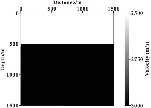
FIGURE 1. A two-layer velocity model.

FIGURE 2

FIGURE 2. The source wavefield snapshot at 0.3 s.

FIGURE 3

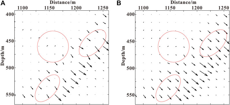
FIGURE 3. The wavefield direction near the reflection interface calculated: (A) based on the Poynting vector; (B) based on the optical flow vector.

FIGURE 4

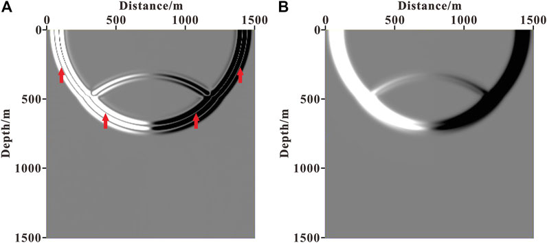
FIGURE 4. Horizontal components: (A) the Poynting vector; (B) the optical flow vector.

FIGURE 5

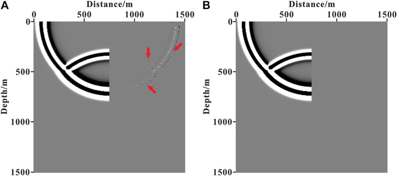
FIGURE 5. Left-going wavefield after decomposition: (A) based on the Poynting vector; (B) based on optical flow vector.

From Figures 3A,B (indicated by the red circle) and Figures 4A,B (indicated by the red arrow), it can be seen that accurately indicating the propagation direction of the wavefield using the Poynting vector is challenging and singular values are prone to appear, whereas the optical flow vector is smoother and the instability phenomenon is avoided effectively. Comparing Figures 5A,B, we can see that for the wavefield decomposition achieved based on the Poynting vector, some other wavefield components as indicated by the arrow appear because the Poynting vector calculation is inaccurate and unstable, whereas the optical flow vector does not generate other wavefield components, so the decomposed wavefield is more accurate.

Angle-Weighted RTM Imaging Based on the Optical Flow Vector

Based on the optical flow vector, we use Eq. 10 to decompose the source and receiver wavefields in the four directions of up, down, left, and right:

$\begin{array}{l}{S}_u\left(x,z,t\right)=\{\begin{array}{l}S\left(x,z,t\right)if{\mathit{P}}_z^o<0\\ 0\end{array}\\ S_d\left(x,z,t\right)=\{\begin{array}{l}S\left(x,z,t\right)if{\mathit{P}}_z^o\ge 0\\ 0\end{array}\\ S_l\left(x,z,t\right)=\{\begin{array}{l}S\left(x,z,t\right)if{\mathit{P}}_x^o<0\\ 0\end{array}\\ S_r\left(x,z,t\right)=\{\begin{array}{l}S\left(x,z,t\right)if{\mathit{P}}_x^o\ge 0\\ 0\end{array}\\ R_u\left(x,z,t\right)=\{\begin{array}{l}R\left(x,z,t\right)if{\mathit{P}}_z^o<0\\ 0\end{array}\\ R_d\left(x,z,t\right)=\{\begin{array}{l}R\left(x,z,t\right)if{\mathit{P}}_z^o\ge 0\\ 0\end{array}\\ R_l\left(x,z,t\right)=\{\begin{array}{l}R\left(x,z,t\right)if{\mathit{P}}_x^o<0\\ 0\end{array}\\ R_r\left(x,z,t\right)=\{\begin{array}{l}R\left(x,z,t\right)if{\mathit{P}}_x^o\ge 0\\ 0\end{array}\end{array},(10)$

where S_u(x, z, t), S_d (x, z, t), S_l (x, z, t), and S_r (x, z, t) denote the up-, down-, left-, and right-going source wavefields, respectively, and R_u (x, z, t), R_d (x, z, t), R_l (x, z, t), and R_r (x, z, t) represent the up-, down-, left-, and right-going wavefields of receivers, respectively.

The decomposed wavefields of both sources and receivers in the opposite direction are selected for imaging separately to avoid migration artifacts (Chen and He, 2014), using the following:

$\begin{array}{l}{I}_{op}\left(x,z\right)=\frac{{\displaystyle \sum _t{S}_u\left(x,z,t\right)R_d\left(x,z,t\right)+{\displaystyle \sum _t{S}_d\left(x,z,t\right)R_u\left(x,z,t\right)}}}{{\displaystyle \sum _t{S}^2\left(x,z,t\right)}}\\ +\frac{+{\displaystyle \sum _t{S}_l\left(x,z,t\right)R_r\left(x,z,t\right)+{\displaystyle \sum _t{S}_r\left(x,z,t\right)R_l\left(x,z,t\right)}}}{{\displaystyle \sum _t{S}^2\left(x,z,t\right)}}\end{array},(11)$

where I_op (x, z) is the optimal stack section. However, in fact, the migration artifacts are mainly distributed in the large-angle region (Yoon and Marfurt, 2006; Zhang et al., 2014; Zhang et al., 2020). Although the method of selecting the wavefields in the opposite direction for imaging can reduce the migration artifacts of 180° or close to 180°, the suppression effect on the migration artifacts coming from other large-angle regions is weak. Moreover, there is also a risk of losing effective information if only the wavefields in the opposite direction are selected for imaging. To address this problem, the reflection angle of each imaging point underground is first calculated based on the optical flow vector. The calculation formula can be defined as follows:

$\theta =\pi -\mathrm{a}\mathrm{r}\cos \left(\frac{{\mathbf{P}}_{\mathbf{S}}^{\mathbf{o}}\left(x,z,t\right)·{\mathbf{P}}_{\mathbf{R}}^{\mathbf{o}}\left(x,z,t\right)}{\left|{\mathbf{P}}_{\mathbf{S}}^{\mathbf{o}}\left(x,z,t\right)\right|\ast \left|{\mathbf{P}}_{\mathbf{R}}^{\mathbf{o}}\left(x,z,t\right)\right|}\right),(12)$

where θ is the reflection angle of each imaging point and P^o_S and P^o_R are the optical flow vectors of the source and receiver wavefields, respectively. Then, an attenuation factor related to the reflection angle is introduced as a weight to generate the optimal stack section, and the final imaging result is obtained according to Eq. 13:

$I\left(x,z\right)=\left(\begin{array}{l}\frac{{\displaystyle \sum _t{S}_u\left(x,z,t\right)R_d\left(x,z,t\right)+{\displaystyle \sum _t{S}_d\left(x,z,t\right)R_u\left(x,z,t\right)}}}{{\displaystyle \sum _t{S}^2\left(x,z,t\right)}}\\ +\frac{+{\displaystyle \sum _t{S}_l\left(x,z,t\right)R_r\left(x,z,t\right)+{\displaystyle \sum _t{S}_r\left(x,z,t\right)R_l\left(x,z,t\right)}}}{{\displaystyle \sum _t{S}^2\left(x,z,t\right)}}\end{array}\right)w\left(\theta \right),(13)$

where I (x, z) is the final imaging result of angle-weighted RTM with wavefield decomposition based on the optical flow vector and w(θ) is the attenuation function, and we choose a cosine-type function as the attenuation function.

The two-layer velocity model in Wavefield Decomposition Based on the Optical Flow Vector is used to test the effect of the angle-weighted imaging method. Figure 6A shows the result of conventional RTM, Figure 6B illustrates the result of RTM with wavefield decomposition based on the Poynting vector, Figure 6C contains the result of RTM with wavefield decomposition based on the optical flow vector, and Figure 6D is the result of angle-weighted RTM with wavefield decomposition based on the optical flow vector.

FIGURE 6

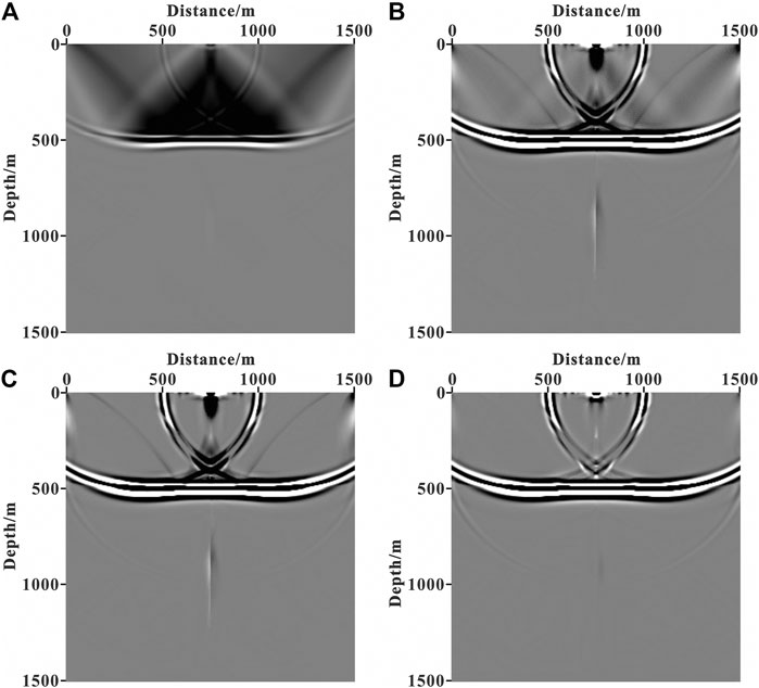
FIGURE 6. The imaging result of RTM: (A) conventional RTM; (B) RTM with wavefield decomposition based on the Poynting vector; (C) RTM with wavefield decomposition based on the optical flow vector; (D) angle-weighted RTM with wavefield decomposition based on the optical flow vector.

There are obvious migration artifacts in the conventional RTM imaging result in Figure 6A. As shown in Figures 6B–D, we can see that most of the migration artifacts are eliminated in the result of RTM with wavefield decomposition based on the Poynting vector. However, due to inaccurate wavefield decomposition, there are still some noises remaining, and as a result of RTM with wavefield decomposition based on the optical flow vector, the migration artifacts are further suppressed. Moreover, the migration artifacts are basically completely suppressed, and the effective structural imaging is highlighted by performing angle weighting processing on the optimal stack section. Therefore, the angle-weighted RTM with wavefield decomposition based on the optical flow vector can produce the accurate imaging of underground structures.

Numerical Test on the Marmousi Model

A region of the Marmousi-II model (as shown in Figure 7) is used to test the imaging accuracy of our method. The size of the model is 6,500 m in length and 3,500 m in depth. The grid spacing is 5 m. There are a total of 101 shots and each shot contains 1,300 receivers. The sampling intervals for the shots and receivers are 65 m and 5 m, respectively. The depths of shots and receivers are both 0 m. A Ricker wavelet with a dominant frequency of 30 Hz is used as the source. The time sampling interval is 0.4 ms and the total recording time is 4 s. The finite-difference accuracy of wavefield continuation is eighth order in space. Figure 8A contains the result of conventional RTM, Figure 8B illustrates the result of RTM with wavefield decomposition based on the Poynting vector, Figure 8C shows the result of RTM with wavefield decomposition based on the optical flow vector, and Figure 8D is the result of angle-weighted RTM with wavefield decomposition based on the optical flow vector.

FIGURE 7

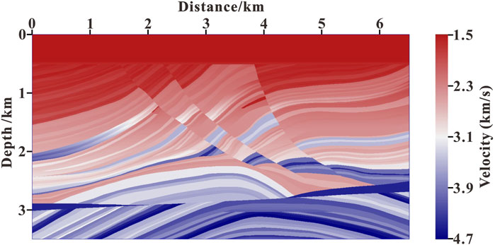
FIGURE 7. The local velocity model of the Marmousi-II model.

FIGURE 8

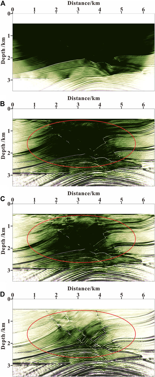
FIGURE 8. RTM section for Marmousi-II model: (A) conventional RTM; (B) RTM with wavefield decomposition based on the Poynting vector; (C) RTM with wavefield decomposition based on the optical flow vector; (D) angle-weighted RTM with wavefield decomposition based on the optical flow vector.

As shown in Figure 8A, the image suffers from low-wavenumber noises. The migration artifacts seriously affect the imaging quality and the real imaging structure is completely concealed. It can be seen from Figures 8B–D that all three methods can significantly suppress migration image noises. However, as shown by the red circle in Figure 8, there are still lots of image noises in Figure 8B, and although the migration artifacts in Figure 8C are further eliminated, a few noises are still left. The noises suppression effect in Figure 8D is the best, the underground structure is the clearest, and the quality of the migration section is greatly improved. Moreover, our attenuation factor puts more weight on the RTM result in the deep part because the reflections generated in the deep part usually have a smaller reflection angle than those in the shallow part for a fixed offset. Therefore, the deep imaging accuracy is further enhanced using our attenuation factor.

Field Marine Seismic Data Imaging

A field marine seismic line in the East China sea is selected for the RTM test. The line involves 1,637 shots, among which shots are arranged on the right side, while receivers are on the left side. A total of 648 receivers are allotted for each shot. The interval between shots is 37.5 m and the interval between receivers is 12.5 m. The depths of shots and receivers are both 12.5 m. The minimum offset is 187.5 m and the maximum recording time of shot gather is 8 s. The finite-difference difference accuracy of wavefield continuation is eighth order in space and second order in time. Meanwhile, the time sampling step is 1 ms. Figure 9 shows the seismic record of the 601st shot. Figure 10 illustrates a source wavelet that is extracted from the original data.

FIGURE 9

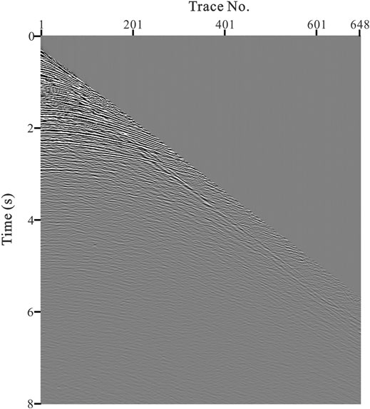
FIGURE 9. The seismic record of the 601st shot.

FIGURE 10

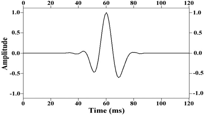
FIGURE 10. Source wavelet.

Figure 11 shows the velocity model of field data, which is obtained by full waveform inversion. Figure 12 illustrates the RTM sections for field marine seismic data (the part ranging from 10 to 70 km is displayed). Among them, Figure 12A is the result of conventional RTM; Figure 12B illustrates the result of RTM with wavefield decomposition based on the Poynting vector; Figure 12C is the result of RTM with wavefield decomposition based on the optical flow vector; Figure 12D shows the result of angle-weighted RTM with wavefield decomposition based on the optical flow vector. From Figure 12A, we can see that there are lots of low-wavenumber noises in the shallow part, as shown by the black dotted circle, which seriously reduces the imaging quality. It can be seen from Figure 12B that low-wavenumber noises are reduced a lot. In Figure 12C, there are fewer noises than in Figure 12B, and in Figure 12D, there are no obvious noises. Therefore, we can conclude that the method in this article can more effectively eliminate low-wavenumber noises compared to other methods and it is suitable for RTM of real data.

FIGURE 11

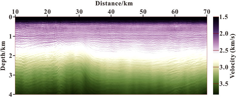
FIGURE 11. Velocity model of field data.

FIGURE 12

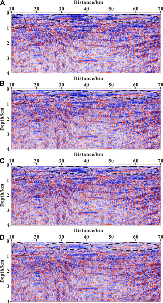
FIGURE 12. RTM section for field marine seismic data: (A) conventional RTM; (B) RTM with wavefield decomposition based on the Poynting vector; (C) RTM with wavefield decomposition based on the optical flow vector; (D) angle-weighted RTM with wavefield decomposition based on the optical flow vector.

Conclusion

The decomposition of source and receiver wavefields can be accurately implemented using the optical flow vector. Then, the cross-correlation imaging sections of one-way propagation components of the forward- and back-propagated wavefields are optimized and stacked. Furthermore, the reflection angle of each imaging point is calculated based on the optical flow vector, and an attenuation factor related to the reflection angle is used as the weight to give the optimal stack images. The numerical experimental results demonstrate the following:

1) The optical flow vector can be used to decompose the wavefield accurately and stably, and RTM with wavefield decomposition based on the optical flow vector can alleviate the effect of low-wavenumber noises effectively.

2) Angle weighting processing can further eliminate large-angle migration artifacts and highlight effective underground structure imaging, thereby significantly improving the imaging accuracy of RTM.

3) The angle-weighted RTM with wavefield decomposition based on the optical flow vector can more effectively eliminate low-wavenumber noises than other methods and it is suitable for RTM of real data.

The proposed method can be applied to elastic-wave RTM and can be further extended to least-squares RTM.

Data Availability Statement

The original contributions presented in the study are included in the article/Supplementary Material; further inquiries can be directed to the corresponding author.

Author Contributions

CX contributed to the writing of the original draft. PS was responsible for conceptualization and project administration. XL was responsible for formal analysis. JT was responsible for software application. SW contributed to the methodology. BZ offered suggestions.

Funding

This research is jointly funded by the National Natural Science Foundation of China (No. 42074138), Fundamental Research Funds for the Central Universities (201964016), and the Major Scientific and Technological Innovation Project of Shandong Province (2019JZZY010803).

Conflict of Interest

The authors declare that the research was conducted in the absence of any commercial or financial relationships that could be construed as a potential conflict of interest.

Publisher’s Note

All claims expressed in this article are solely those of the authors and do not necessarily represent those of their affiliated organizations, or those of the publisher, the editors and the reviewers. Any product that may be evaluated in this article, or claim that may be made by its manufacturer, is not guaranteed or endorsed by the publisher.

References

Baysal, E., Kosloff, D. D., and Sherwood, J. W. C. (1984). A Two‐way Nonreflecting Wave Equation. Geophysics 49, 132–141. doi:10.1190/1.1441644

CrossRef Full Text | Google Scholar

Baysal, E., Kosloff, D. D., and Sherwood, J. W. C. (1983). Reverse Time Migration. Geophysics 48, 1514–1524. doi:10.1190/1.1441434

CrossRef Full Text | Google Scholar

Berenger, J.-P. (1994). A Perfectly Matched Layer for the Absorption of Electromagnetic Waves. J. Comput. Phys. 114, 185–200. doi:10.1006/jcph.1994.1159

CrossRef Full Text | Google Scholar

Chen, T., and He, B.-S. (2014). A Normalized Wavefield Separation Cross-Correlation Imaging Condition for Reverse Time Migration Based on Poynting Vector. Appl. Geophys. 11, 158–166. doi:10.1007/s11770-014-0441-5

CrossRef Full Text | Google Scholar

Collino, F., and Tsogka, C. (2001). Application of the Perfectly Matched Absorbing Layer Model to the Linear Elastodynamic Problem in Anisotropic Heterogeneous media. Geophysics 66, 294–307. doi:10.1190/1.1444908

CrossRef Full Text | Google Scholar

Du, Q., Zhu, Y., and Ba, J. (2012). Polarity Reversal Correction for Elastic Reverse Time Migration. Geophysics 77, S31–S41. doi:10.1190/GEO2011-0348.1

CrossRef Full Text | Google Scholar

Du, Q. Z., Zhu, Y. T., Zhang, M. Q., and Gong, X. F. (2013). A Study on the Strategy of Low Wavenumber Noise Suppression for Prestack Reverse-Time Depth Migration. Chin. J. Geophys. 56, 2391–2401. doi:10.6038/cjg20130725

CrossRef Full Text | Google Scholar

Duan, Y., and Sava, P. (2015). Scalar Imaging Condition for Elastic Reverse Time Migration. Geophysics 80, S127–S136. doi:10.1190/GEO2014-0453.1

CrossRef Full Text | Google Scholar

Fee, D., Toney, L., Kim, K., Sanderson, R. W., Iezzi, A. M., Matoza, R. S., et al. (2021). Local Explosion Detection and Infrasound Localization by Reverse Time Migration Using 3-D Finite-Difference Wave Propagation. Front. Earth Sci. 9, 620813. doi:10.3389/feart.2021.620813

CrossRef Full Text | Google Scholar

Fei, T. W., Luo, Y., Yang, J., Liu, H., and Qin, F. (2015). Removing False Images in Reverse Time Migration: The Concept of De-primary. Geophysics 80, S237–S244. doi:10.1190/GEO2015-0289.1

CrossRef Full Text | Google Scholar

Gong, T., Nguyen, B. D., and McMechan, G. A. (2016). Polarized Wavefield Magnitudes with Optical Flow for Elastic Angle-Domain Common-Image Gathers. Geophysics 81, S239–S251. doi:10.1190/GEO2015-0518.1

CrossRef Full Text | Google Scholar

Horn, B. K. P., and Schunck, B. G. (1981). Determining Optical Flow. Artif. intelligence 17, 185–203. doi:10.1016/0004-3702(81)90024-2

CrossRef Full Text | Google Scholar

Hu, C., Albertin, U., and Johnsen, T. (2014). Optical Flow Equation Based Imaging Condition for Elastic Reverse Time Migration. Ann. Internat Mtg.Soc. Expi. Geophys. Expanded Abstr. 84, 3877–3881. doi:10.1190/segam2014-0140.1

CrossRef Full Text | Google Scholar

Li, K.-R., and He, B.-S. (2020). Extraction of P- and S-Wave Angle-Domain Common-Image Gathers Based on First-Order Velocity-Dilatation-Rotation Equations. Appl. Geophys. 17, 92–102. doi:10.1007/s11770-019-0799-5

CrossRef Full Text | Google Scholar

Liu, F., Zhang, G., Morton, S. A., and Leveille, J. P. (2011). An Effective Imaging Condition for Reverse-Time Migration Using Wavefield Decomposition. Geophysics 76, S29–S39. doi:10.1190/1.3533914

CrossRef Full Text | Google Scholar

Liu, Q. (2019). Dip-angle Image Gather Computation Using the Poynting Vector in Elastic Reverse Time Migration and Their Application for Noise Suppression. Geophysics 84, S159–S169. doi:10.1190/GEO2018-0229.1

CrossRef Full Text | Google Scholar

Lucas, B. D., and Kanade, T. (1981). “An Iterative Image Registration Technique with an Application to Stereo Vision,” in Proceedings of the 7th International Joint Conference on Artificial Intelligence, San Francisco, CA, United States (San Mateo, CA: Morgan Kaufmann Publishers Inc.), 674–679.

Google Scholar

McMechan, G. A. (1983). Migration by Extrapolation of Time-dependent Boundary Values. Geophys. Prospect 31, 413–420. doi:10.1111/j.1365-2478.1983.tb01060.x

CrossRef Full Text | Google Scholar

Mulder, W. A., and Plessix, R. E. (2004). A Comparison between One‐way and Two‐way Wave‐equation Migration. Geophysics 69, 1491–1504. doi:10.1190/1.1836822

CrossRef Full Text | Google Scholar

Oh, J.-W., Kalita, M., and Alkhalifah, T. (2018). 3D Elastic Full-Waveform Inversion Using P-Wave Excitation Amplitude: Application to Ocean Bottom cable Field Data. Geophysics 83, R129–R140. doi:10.1190/GEO2017-0236.1

CrossRef Full Text | Google Scholar

Poynting, J. H. (1884). XV. On the Transfer of Energy in the Electromagnetic Field. Phil. Trans. R. Soc. 175, 343–361. doi:10.1098/rspl.1883.009610.1098/rstl.1884.0016

CrossRef Full Text | Google Scholar

Qu, Y., Guan, Z., Li, J., and Li, Z. (2020). Fluid-solid Coupled Full-Waveform Inversion in the Curvilinear Coordinates for Ocean-Bottom cable Data. Geophysics 85, R113–R133. doi:10.1190/GEO2018-0743.1

CrossRef Full Text | Google Scholar

Song, P. (2005). Accurate Absorbing Boundary Conditions and Reverse-Time Migration of Acoustic Wave Equation Using Non-reflecting Recursive Algorithm: [Master’s Thesis]. Qingdao: Ocean University of China.

Google Scholar

Sun, D., Jiao, K., Cheng, X., and Vigh, D. (2015). Compensating for Source and Receiver Ghost Effects in Full Waveform Inversion and Reverse Time Migration for marine Streamer Data. Geophys. J. Int. 201, 1507–1521. doi:10.1093/gji/ggv089

CrossRef Full Text | Google Scholar

Tang, C., McMechan, G. A., and Wang, D. (2017). Two Algorithms to Stabilize Multidirectional Poynting Vectors for Calculating Angle Gathers from Reverse Time Migration. Geophysics 82, S129–S141. doi:10.1190/GEO2016-0101.1

CrossRef Full Text | Google Scholar

Wang, P. F., and He, B. S. (2017). Vector Field Dot Product Cross-Correlation Imaging Based on 3D Elastic Wave Separation. Oil Geophys. Prospecting 52, 477–483. doi:10.1380/j.cnki.issn.1000-7210.2017.03.009

CrossRef Full Text | Google Scholar

Wang, X. Y., Zhang, J. J., Xu, H. Q., and Tian, B. Q. (2021). Least-squares Reverse Time Migration with Wavefield Decomposition Based on the Poynting Vector. Chin. J. Geophys. 64, 645–655. doi:10.06038/cjg2021O0120

CrossRef Full Text | Google Scholar

Wang, Y. B., Zheng, Y. K., Xue, Q. F., Chang, X., Fei, W., and Luo, Y. (2016). Reverse Time Migration with Hilbert Transform Based Full Wavefield Decomposition. Chin. J. Geophys. 59, 4200–4211. doi:10.6038/cjg20161122

CrossRef Full Text | Google Scholar

Whitmore, N. D. (1983). Iterative Depth Migration by Backward Time Propagation. Ann. Internat Mtg.Soc. Expi. Geophys. Expanded Abstr. 53, 382–385. doi:10.1190/1.1893867

CrossRef Full Text | Google Scholar

Wu, C. L., Wang, H. Z., Feng, B., and Sheng, S. (2021). RTM Angle Gathers Based on the Combining Local and Global (CLG) Optical Flow Method and Wavefield Decomposition Method. Chin. J. Geophys. 64, 1375–1388. doi:10.6038/cjg2021O0088Yoon

CrossRef Full Text | Google Scholar

Yoon, K., and Marfurt, K. J. (2006). Reverse-time Migration Using the Poynting Vector. Exploration Geophys. 37, 102–107. doi:10.1071/EG06102

CrossRef Full Text | Google Scholar

Zhang, D., Fei, T. W., and Luo, Y. (2018). Improving Reverse Time Migration Angle Gathers by Efficient Wavefield Separation. Geophysics 83, S187–S195. doi:10.1190/GEO2017-0348.1

CrossRef Full Text | Google Scholar

Zhang, L., Liu, Y., Jia, W., and Wang, J. (2020). Suppressing Residual Low-Frequency Noise in VSP Reverse Time Migration by Combining Wavefield Decomposition Imaging Condition with Poynting Vector Filtering. Exploration Geophys. 52, 235–244. doi:10.1080/08123985.2020.1804298

CrossRef Full Text | Google Scholar

Zhang, W., and Shen, Y. (2010). Unsplit Complex Frequency-Shifted PML Implementation Using Auxiliary Differential Equations for Seismic Wave Modeling. Geophysics 75, T141–T154. doi:10.1190/1.3463431

CrossRef Full Text | Google Scholar

Zhang, Y., and Sun, J. (2009). Practical Issues in Reverse Time Migration: True Amplitude Gathers, Noise Removal and Harmonic Source Encodingnoise Removal and Harmonic-Source Encoding. First Break 27, 53–59. doi:10.3997/1365-2397.2009002

CrossRef Full Text | Google Scholar

Zhang, Q. (2014). RTM Angle Gathers and Specular Filter (SF) RTM Using Optical Flow. Ann. Internat Mtg.Soc. Expi. Geophys. Expanded Abstr. 84, 3816–3820. doi:10.1190/segam2014-0792.1

CrossRef Full Text | Google Scholar