 Pietro Milillo
 Gianfranco Sacco3
 Diego Di Martire
- 1Department of Civil and Environmental Engineering, Cullen College of Engineering, University of Houston, Houston, TX, United States
- 2German Aerospace Center (DLR), Microwaves and Radar Institute, Munich, Germany
- 3NASA Jet Propulsion Laboratory, California Institute of Technology, Pasadena, CA, United States
- 4Department of Earth Sciences, Environment and Resources, University Federico II, Naples, Italy
We present a neural network-based method to detect anomalies in time-dependent surface deformation fields given a set of geodetic images of displacements collected from multiple viewing geometries. The presented methodology is based on a supervised classification approach using combinations of line of sight multitemporal, multi-geometry interferometric synthetic aperture radar (InSAR) time series of displacements. We demonstrate this method with a set of 170 million time series of surface deformation generated for the entire Italian territory and derived from ERS, ENVISAT, and COSMO-SkyMed Synthetic Aperture Radar satellite constellations. We create a training dataset that has been compared with independently validated data and current state-of-the-art classification techniques. Compared to state-of-the-art algorithms, the presented framework provides increased detection accuracy, precision, recall, and reduced processing times for critical infrastructure and landslide monitoring. This study highlights how the proposed approach can accelerate the anomalous points identification step by up to 147 times compared to analytical and other artificial intelligence methods and can be theoretically extended to other geodetic measurements such as GPS, leveling data, or extensometers. Our results indicate that the proposed approach would make the anomaly identification post-processing times negligible when compared to the InSAR time-series processing.
Introduction
Synthetic aperture radar (SAR)-based geodetic imaging has revolutionized Earth science research in disciplines such as solid Earth, ecosystems, and cryosphere. Yet, the ability to effectively utilize SAR data for research, long-term monitoring of extensive spatial areas of interests (AOIs), and rapid hazard response has been limited due to processing complexity, data volume sizes, and latencies in the end-to-end process. For example, barriers in urgent response include the lack of automated data triggers from forecasts, the need for specialized processing parameters that currently rely on expert intervention, and the manual delivery of actionable science data products to the decision support communities. Decision support products, which often are most useful if they are generated rapidly and with simplified information (e.g., damaged or not damaged or accelerating or not accelerating), often require change detection-based approaches utilizing the before and after event scenes to be processed often with threshold values set ad hoc on the underlying SAR processing parameters values (Refice et al., 2014; Yun et al., 2015; Confuorto et al., 2017; Milillo et al., 2018; Karimzadeh and Matsuoka, 2018; Raspini et al., 2018; Giardina et al., 2019). These steps requiring a human-in-the-loop have become a bottleneck for rapid and reliable exploitation of geodetic data for both long-term monitoring and event response with SAR data.
If done correctly, SAR data can also be used to monitor for events such as volcano inflation or precursory signals to landslide events and infrastructure collapse (Sousa and Bastos, 2013; Milillo et al., 2015; Bonì et al., 2018; Intrieri et al., 2018; Selvakumaran et al., 2018; Burrows et al., 2019; Carlà et al., 2019; Gaddes et al., 2019; Milillo et al., 2019; Infante et al., 2019). Automating these time domain-based feature detection methods have even larger barriers due to processing of large temporal co-registered data stacks, processing complexity, as well as human expertise needed to assess the time domain signals. With the launch of European Space Agency (ESA)’s Sentinel 1A and 1B providing open access to near-global SAR data, the number of AOI that can be continuously monitored as well as AOIs for disaster response have grown significantly.
The all-weather multi-temporal characteristics of SAR make its products suitable for structural health monitoring systems, especially in areas where in situ measurements are not feasible or not cost-effective. This provides opportunities to exploit multi-temporal data stacks for long-term monitoring such as those from earthquake events, flooding events, volcanoes, landslides, and infrastructure monitoring (Ito et al., 2000; Ngo et al., 2018; Anantrasirichai et al., 2019; Ji et al., 2019). Here, we focus on InSAR surface displacement time-series post-processing aspects related to the creation of an early warning system.
Several machine learning-based technology demonstrations have been developed to help classify events and other features from Earth observation data. Though many prior classification approaches focused on land-use and ground-based object classification (Lazebnik et al., 2006; Cheriyadat, 2014; Penatti et al., 2015), newer methods for machine learning have focused on natural phenomena detection. More recently, convolutional neural networks (CNNs) have been applied to phenomena-based Earth science image classification (Maskey et al., 2017). Machine learning approaches for Earth science data have typically been applied on these types of single-scene feature detection. Now, with more availability of low-latency and global multi-temporal remote sensing data, opportunities exist to exploit time-dependent features of highly temporal Earth science observations. Unlike the current state-of-the-art pairwise change detection techniques, multi-temporal spatial prediction techniques that leverage long-term historical observations yield more accurate and interpretable predictions (Yun et al., 2015).
Literature studies investigate the automatic classification of InSAR time series of surface deformation (Berti et al., 2013; Chang and Hanssen, 2016; Tomàs et al., 2019; Fiorentini et al., 2020) (Table 1). These studies propose methods focused mainly on conditional sequence of statistical tests (Berti et al., 2013) or probabilistic multiple hypotheses testing (Chang and Hanssen, 2016) based on a pre-defined set of known functions that could better represent the temporal behavior of a time series of surface deformation. Existing approaches have been mainly developed as post-processing tools for shedding new light on the physical behavior of landslides (Berti et al., 2013) and to provide insights into the standardization of InSAR time-series products (Chang and Hanssen, 2016). Other studies, instead, focus on the definition of anomalous points or areas and how they can be identified in an InSAR time series of surface displacement (Raspini et al., 2018; Meisina et al., 2008). However, several limitations can influence the effectiveness of these methods (see Methods and Algorithms) including (1) the manual ad hoc thresholds inferred over the specific region of interest; (2) the absence of a parameter taking into consideration the time-series noise level; (3) the time required by the algorithm for a full analysis of a single region; and (4) the overall time-series length of at least 1 year [i.e., more appropriate for a yearly analysis leading to increased ghost anomalies when used in a near-real time response mode or if the signal is affected by seasonal periodic trends (Chaussard et al., 2017). The effectivity of the proposed methodology depends not only on the chosen thresholds, but also on the data quality and data take acquisition rate (Moretto et al., 2017). Other limiting factors are related to the limited automation [30] and the high number of requested input features such as topographic wetness index, drainage capacity of the soil, erosion susceptibility, and wind exposition (Fiorentini et al., 2020) that make the algorithm less generic and inapplicable over areas where all the aforementioned input features are not available. Existing studies only couple a maximum of two of the following aspects related to (1) large-scale statistical analyses; (2) the use of ground-truth data based on the analysis of optical/radar data and field inspections; and (3) detection of anomalies in the satellite data. As an example, the analyzed synthetic and real dataset are only extended to a local (Chang and Hanssen, 2016; Tomàs et al., 2019; Fiorentini et al., 2020) or regional scale (Raspini et al., 2018) and do not exceed 750,000 time series analyzed at a maximum speed rate of 32 samples/s (Chang and Hanssen, 2016).
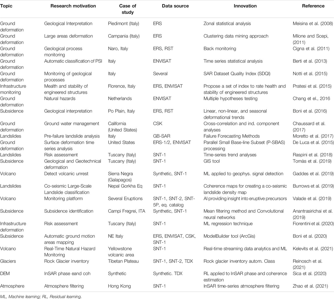
TABLE 1. Revised literature of the main classification approaches applied to InSAR.
In this paper, we further develop this topic and present an automated large-scale machine learning analysis framework of multi-temporal transient detection and precursory signal analysis of Interferometric SAR (InSAR) time series of surface deformation. We exploit a dataset of 170 million time series of InSAR surface deformation and highlight the advantages of the proposed framework for shortening post-processing times of ESA’s ERS, Envisat, and Sentinel-1A/B and the Italian space agency’s (ASI) COSMO-SkyMed data archives. Our training dataset is based on data validated by an independent study (Di Martire et al., 2017) using field analysis and remote sensing data. As explained in detail in the conclusions of this paper, the proposed experiments can be considered an initial proof of concept to provide a preliminary early warning system capable of detecting anomalous points in InSAR time series of surface displacement. The simplicity of the proposed method when compared to previous more sophisticated approaches (Berti et al., 2013; Chang and Hanssen, 2016; Fiorentini et al., 2020; Tomàs et al., 2019) constitutes a key advantage in terms of processing time, which is fundamental when looking at deformation assessment in near-real time.
The discussion is organized as follows. Methods and Algorithms describes the methodology and algorithms focusing on the InSAR time-series analysis, anomalies detection, and the neural network framework. Dataset presents the dataset and the model optimization. Results and Discussion describes the results and comparisons with independent datasets including state-of-the-art classification approaches. Conclusion and Perspectives describes the potential for our technique to improve the understanding dynamic processes characterizing the field of Earth science and its applications.
Methods and Algorithms
In this section, we describe details of the different methodologies adopted for detecting anomalies. Specifically, we use an analytical method already proposed in literature (Raspini et al., 2018), a state-of-the-art random forest algorithm (Breiman, 2001), and the proposed neural network approach. An updated landslide inventory map produced through the Landslide Detection Integrated System (LADIS) (Di Martire et al., 2017) together with the CSK dataset presented in Costantini et al. (2017) is used as input for the analytical model (Raspini et al., 2018) (see Dataset). The output dataset is formed by data tagged as “Signal/Anomaly or noise/no anomaly” and is used for training the Random Forest and the proposed neural network (Breiman, 2001). Figure 1 provides details of the data processing workflow and the contribution of each dataset to the processing workflow.
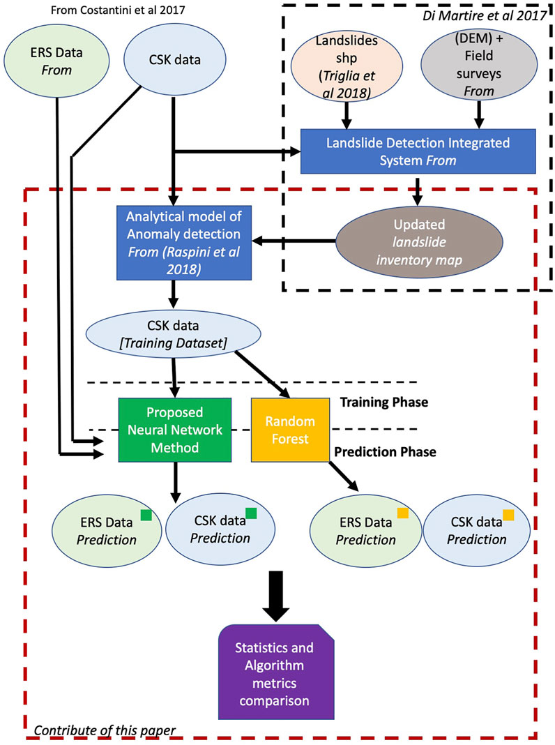
FIGURE 1. Data Processing workflow scheme adopted in this study. The contribution of reference (Di Martire et al., 2017) is highlighted as a black dashed line, whereas the contribution of this paper is highlighted by a red dashed line. Our Training dataset is formed by anomalous points [as described in (Raspini et al., 2018)] belonging to the CSK dataset falling within a landslide area extracted from the landslide inventory map described in Di Martire et al. (2017). These points are then used to train the Neural network and the Random Forset classifiers, which are then applied to the entire dataset.
InSAR Time-Series Analysis
SAR is a coherent active sensor operating in the microwave band that exploits relative motion between antenna and target in order to obtain a finer spatial resolution in the flight direction (Azimuth) exploiting the Doppler effect. In this way, it is possible to synthetize a kilometer-scale antenna with a several-meter real antenna (typically 10 m). In the direction transverse to the direction of flight (range), pulse modulation technique is used in order to increase spatial resolution. Because of its coherent nature, SAR can exploit both amplitude and phase of an electromagnetic signal. SAR data can be seen as a bidimensional array containing both phase and amplitude information related to the backscattered electromagnetic radiation. SAR interferometry (InSAR) consists of the coherent cross-multiplication of two coherent signals and extraction of the phase component. The repeat pass interferometric phase depends on the ground changes that occurred within the time acquisition interval of two acquisitions. This technique is called differential SAR interferometry (DInSAR) and is a powerful tool for detecting surface changes. Multitemporal analysis extends InSAR technique by combining several acquisitions highlighting the temporal behavior of the relative displacement between each acquisition along the satellite line of sight (LOS). In this study, we used pre-processed data according to the PS-like approach described in Costantini et al. (2017).
Anomaly Detection Using an Analytical Model
Once a time series of surface deformation has been generated using a multi-temporal InSAR approach, each time-series measurement point is systematically analyzed in order to identify changes in the deformation pattern and to highlight “anomalous points” (Raspini et al., 2018). In our study, we adopt the definition of “anomalous point” as described by Raspini et al. (2018), i.e., a measurement that changes its velocity (VC threshold) by 10 mm/year between subsequent epochs spanning 150 days (TW time window). This method is based on the temporal under-sampling of displacement time series, and once the VC and TW arbitrary thresholds are set, the analysis is then carried out automatically according to the following procedure reported in Raspini et al. (2018): “
• within the entire monitoring interval (T0–Tn), a temporal window of 150 days is set in the final part of the TS (Tn–150–Tn), allowing the sampling of two different sub-intervals within the time series, i.e., the Historical (H) (T0–Tn–150) and the Recent (R) intervals (Tn–150–Tn).
• the TS of deformation within the sub-interval R is analyzed to identify any potential deviations that occurred during the monitoring period Tn–150–Tn, with respect to the previous part of the TS;
• when a change in the deformation pattern is identified, a breaking point, Tb is defined;
• the average deformation rates for each subsample (i.e., v1 in the time interval T0–Tb and v2 in the time interval Tb–Tn) are recalculated as simple linear regressions on ground deformation data;
• when |ΔV| = v2−v1 > 10 mm/yr (velocity threshold, THR), an anomalous point is highlighted.”
The analytical method is extremely simple and has been applied over the Tuscany region in Italy (Raspini et al., 2018) in order to produce warning bulletins. We run the analytical model and all the proposed algorithms on MacBook Pro with a 2.4-GHz Intel Core i9 processor and a 32-Gb 2400-MHz DDR4 RAM. We found the inference speed of the analytical model to be 5.1 × 10⁵ samples/s.
Random Forest Classification
Random Forest (Breiman, 2001) is a powerful ensemble algorithm used for regression and classification problems where a set of randomly generated decision trees are trained separately, and a decision is made based on majority voting. One of the several appeals of this technique is that the user could rely on domain specific knowledge in engineering the input features and have a better physical interpretation of the results based on the relative importance that the algorithm assigns to each of them. We performed two sets of experiments where we used engineered features in one and the entire time series was utilized in another. In the first set of experiments, we used the following features (ad hoc features):
• Mean and standard deviation of the time-series displacements.
• Mean and standard deviation of the time-series velocity.
• Mean and standard deviation of the time-series acceleration.
• The maximum absolute displacement in within one-third, two-thirds, and the whole time series.
The results of the different experiments are presented in Results and Discussion. For the sake of clarity, we report here the definition of each metrics: Precision is the ratio between true positives (TP) and the sum of true positives and false positives (FP). Precision attempts to answer the following question: What proportion of positive identifications was actually correct? Recall is the ratio between TP and the sum of TP and false negatives (FN). Recall attempts to answer the following question: what proportion of actual positives was identified correctly? Accuracy is the ratio between the sum of TP and the true negatives (TN) and the sum of TP + TN + FP + FN. The inference speed is simply the number of single time series of 101 samples that can be analyzed within one second.
Proposed Neural Network Approach
Neural Networks (NNs) (Schmidhuber, 2015) have seen a revival in the past decade thanks to the invention of new techniques for normalization (Ioffe and Szegedy, 2015), regularization (Hinton et al., 2012), and new activations functions (for instance, Rectified Linear Unit or ReLU) that improved their overall performance and allowed to train deeper topology. Because of the ability to learn complex patterns, NNs are good candidates to tackle the landslides classification problem. In our experiment, we used a simple two-layer fully connected NN with dropout and batch normalization and cross entropy for loss function (see Table 2). We adopted the Batch Normalization (BN) described by Sergey Ioffe and Christian Szegedy in order to improve the performance of the neural network (Ioffe and Szegedy, 2015). The NN described in Table 1 was implemented using TensorFlow (Shukla, 2018). Because of the unbalanced dataset, the size of the batch resulted in an important hyperparameter. We obtained the best performance for a batch size of 2048, whereas smaller batch sizes resulted in an unstable loss function. The selection of the best model was made by checkpointing the state of the model with the highest F1 score during the validation step. After few iterations, we converged to the model in Table 2.
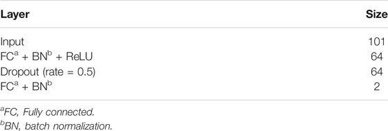
TABLE 2. Description of the adopted neural network model.
Dataset
In this section, we describe how the training and testing datasets are generated and how the different experiments are set up. We use data from the Non-ordinary Plan of Environmental Remote Sensing (Piano Straordinario di Telerilevamento Ambientale) financed by the Italian Ministry of the Environment (Ministero dell’Ambiente e della Tutela del Territorio e del Mare—MATTTM), which has the goal of mapping and preventing geo-hazards within the Italian territory (Costantini et al., 2017). The datasets include 20,000 SAR images acquired between 1992 and 2014 over the whole Italian Territory. Specifically, a global coverage of the Italian territory has been provided between 1992 and 2000 by the ERS-1/2 data while ENVISAT data have been used to cover the time-span 2002–2010 (Figure 2). This dataset comprises a database of 40 million PS points and 2 billion displacement measurements. From 2011 to 2014, a hundred COSMO-SkyMed (CSK) data stacks acquired in ascending and descending geometries have been processed over selected areas of the Italian territory (Figure 2). The CSK dataset provided 130 million PS Points and 6 billion displacement measurements. To our knowledge, this is the largest highly curated dataset freely available through the Geoportale Nazionale (National Geoportal), which is a publishing platform also containing geospatial information related to landslide risk (Di Martire et al., 2017; Trigila and Iadanza, 2018). Further details of the satellite data used in this study can be found in Table 3. We used a validated landslide catalogue from Trigila and Iadanza (2018) as an additional ancillary dataset in order to start the data preparation process and the NN initial training. The landslide shapefile data consist in a highly curated dataset validated by independent studies (Di Martire et al., 2017). Further information related to the dataset used in this study and the ground-based validation technique used for generating the landslide ground truth can be found in Costantini et al. (2017), Di Martire et al. (2017), and Trigila and Iadanza (2018).
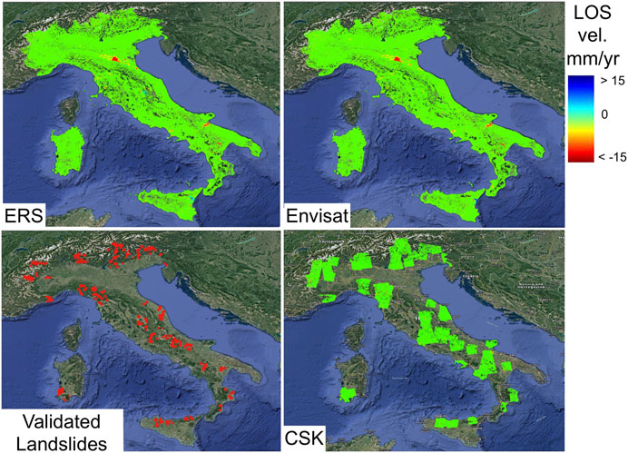
FIGURE 2. Multi-temporal time-series dataset used in this study. The Validated Landslide areas as presented in Di Martire et al. (2017) have been used to subsample the CSK dataset and create a validated training dataset.

TABLE 3. Input CSK, ERS and ENVISAT data characteristics adapted from Costantini et al. (2017) and Di Martire et al. (2017).
Our initial dataset consisted of a large-scale surface displacement time-series map of the Italian peninsula (Figure 2). Separately, we were provided a set of shapefiles with the polygons circumscribing the regions where landslides were manually identified (Di Martire et al., 2017). One challenge we had to face was the fact that the polygons (Figure 2 validated landslides) represented a best estimate of the region that was affected by a landslide, but in actuality, not all the PS time series showed a pattern corresponding necessarily to an actual active accelerating landslide [i.e., not all points within a landslide polygon would be possibly classified as “anomalous” as defined in our analytical model (Raspini et al., 2018)]. As an example, there could be landslides moving toward a direction perpendicular to the satellite LOS (i.e., the satellite-based time series of displacement is insensitive to the direction of motion perpendicular to the LOS). Another example could be related to the fact that the landslide LOS deformation could simply be steady without showing changes over time. On the other hand, the prior knowledge that a landslide has been identified in the area allows the use of the analytical model described in Raspini et al. (2018) Anomaly Detection Using an Analytical Model to classify the time-series points within the polygons as a positive signal (i.e., accelerating landslide) or not. Using the CSK dataset as training together with the approach described in Anomaly Detection Using an Analytical Model, we were able to identify almost 560,000 positive signals (Persistent Scatterers points) within the polygons identified by the landslide detection integrated system (based on field surveys occurring at the same time of the CSK data acquisition time) (Di Martire et al., 2017). The negative signals were similarly identified by considering PS that were randomly selected and that were not part of any of the polygons provided to us and for which the analytic model provided a negative signal. The ensemble of the positive signals and the negative signals represent our gold standard that will be used to train and validate our neural networks to identify anomalous deformation patterns. Since landslides are rare events, the nature of the problem is highly unbalanced and the chance of selecting an unidentified (i.e., not included in the shape files) positive signal and wrongly classify it as a negative signal are very small. To reflect the data distribution, we created a training set with 16% of positives (448,000 positive signal persistent scatterers points) and 84% of negatives (2,352,000 negative signals) and a testing set with 4% of positives (112,000 positive signals persistent scatterers points) and 96% of negatives (2,688,000 negative signals). We did not perform randomization before performing the aforementioned splitting because PS that are in proximity of each other could be highly correlated (i.e., temporal displacement might look very similar). We avoided the randomization step also to avoid leaking of some training data into the test data. This step was performed in order to ensure the two datasets originate from separate physical regions. Because the time series of displacement were not all of the same length, we interpolate them and made them of length 101, resampling them to constant steps.
Results and Discussion
We provide in all our neural network experiments the same gold standard dataset described in Dataset. Two independent sets of 2,8000,000 persistent scatterers points were used as training and validation. The results of the NN anomalies classification of the ERS dataset are presented in Figure 3. The main criteria adopted for model selections were accuracy and inference speed. The second criterion becomes critical when developing a system that is meant for large-scale real-time monitoring. The accuracies and inference speed for the NN experiment applied on the test dataset are shown in Table 4. Given that the problem might be thought as a multi-objective one (optimize accuracy and inference speed), we used Random Forest (RF) with the intent of devising a model that would possibly outperform our first attempt using NN. We performed a first set of experiments using the features previously described in Random Forest Classification and changing the number of trees adopted. We used the software package skit-learn (Pedregosa et al., 2011) and specifically the Random Forest Classifier. The results of the RF classifier using ad hoc features are summarized in Table 5. As it can be seen, limiting the model to 100 trees is sufficient to reach a performance comparable to the more complex model with 500 trees with a higher inference speed. However, the NN model outperforms the RF models presented in Table 4 on both metrics, i.e., accuracy and speed. In our second set of experiments, we did not engineer the features (i.e., we do not calculate the ad hoc features a priori) and instead we provided to the RF model the same inputs as for the NN, i.e., the 101 elements time series. The results are listed in Table 6.
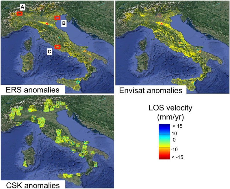
FIGURE 3. Anomalies/Positive signals identified by the Neural Network (NN) algorithm over the entire Italian territory. These points indicate areas where a change in deformation larger than 10 mm/year has been detected during the observation period. Red boxes represent areas shown in Figure 4 (box A and B) and Figure 5 (box C). The CSK ERS and Envisat data have been analyzed separately.

TABLE 4. Results from the neural network experiment.
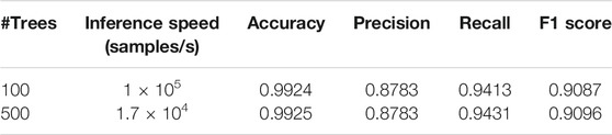
TABLE 5. Results from different experiments using Random Forest Classifier and ad hoc features.
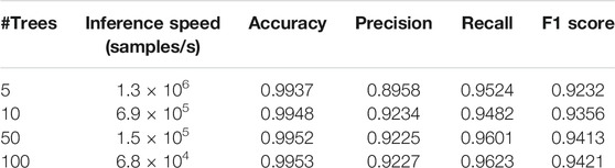
TABLE 6. Results from different experiments using Random Forest Classifier without engineered features.
It can be seen that the 50- and 100-tree models have very similar accuracy. On the other hand, the 5- and 10-tree models have lower precision or recall, respectively, most likely due to a larger variance given the smaller number of trees available. The RF algorithm also provides the importance of each feature, namely, what weight each feature contributes to the final prediction. Since the input to the algorithm is the actual time series, each time step represents a feature. Table 7 shows the nine most important features of the best-performing RF algorithm. As it can be seen, the algorithm relies mostly on the later time steps in the time series to make a prediction. This is expected since the later time steps are an indication of an anomalous point as defined in Raspini et al. (2018) in Anomaly detection using an analytical model.
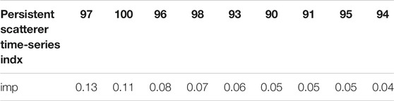
TABLE 7. Most important features when using the whole time series as input to the RFmodel without engineered features.
Random Forest and Neural Network Comparative Analysis
A comparison between the RF models and the NN in terms of inference speed, accuracy, precision, and recall provides detailed insights into the characteristics of each method. Given the results shown in Tables 4–7, we highlight that the NN model can be considered the fastest one outperforming the second fastest (RF with five trees without engineered features) by a factor of 2. In terms of accuracy the RF model with 100 (RF100) trees without engineered features outperforms the RF with 50 trees (RF50) without engineered features and the NN model by 0.01% and 0.02%, respectively. In terms of precision, the RF model with 10 trees without engineered features outperforms the RF100 and NN by 0.006% and 0.017%, respectively. The NN model provides the best recall parameter (0.9705) compared to the RF100 and RF50, which perform 0.82% and 1% worse, respectively.
Numerically speaking, there is no clear “winner”, and all depends on comparison metrics we are more interested into. Given our problem (i.e., we are trying to develop a global near real-time large-scale monitoring system for early detection of “deformation anomalies”), inference time is important. The RF five-tree model is the fastest one among the RF models, but its accuracy is actually the worst if compared to the RF models without engineered features. Moreover, the NN model yields more false positives (lower precision) and less false negatives (higher recall) compared to the best of the RF models. Given the nature of the problem, a false positive implies that after the classification, an expert human operator will spend some extra time to assess the true state of the signal (in this case, not a landslide predicted as landslide). On the other hand, mistaking a true landslide as a negative event could have catastrophic consequences including the loss of human lives.
Neural Network as an Exploratory Tool
Our results show that signals can also be identified by all networks in areas not characterized by landslide risk. As an example, anomalies in time series of surface displacement were found over urban areas and infrastructures. Figure 4 shows time series of points located over infrastructures showing signs of distress (Figures 4F, 5B,F,H) and displacement characterizing landslides (Figures 4B–E). As can be noticed, the deformation patterns are very similar highlighting how, despite the entire training set has been based on time series representing accelerating landslides/no landslides, the network is sensitive to additional physical phenomena such as signs of distress characterizing infrastructure. This feature is based on the intrinsic simplicity of the proposed NN approach (i.e., not taking into consideration land type or terrain properties). Because we trained the algorithm with X-band data, it is also interesting to examine the results of the network over an area covered by both X-Band (CSK) and C-band (ERS, Envisat) time series of surface deformation (Figure 5). The main differences between time series generated using X and C band is related to the time span covered by both time series, the accuracy of the final product, and the different contributions of the noise to the phase signal. As an example, unwrapping errors in a C-band (5.6 cm wavelength) time series would show up as steps or “jumps” of 2.8 cm away or towards the LOS vector whereas the same error would correspond to a 1.5-cm phase “jump” in X-band (3 cm wavelength) time series of surface deformation. Figure 5D shows an anomaly detected by the NN algorithm in the C-Band Envisat dataset, which is caused by an unwrapping error of the dataset presented in Costantini et al. (2017). This example shows how the proposed algorithm is sensitive to unwrapping errors at C-band even if it has been trained with X-band data. This result is expected since the time series in Figure 5D falls within the definition of anomalous point as described in Anomaly Detection Using an Analytical Model. Another interesting result is related to the amount of identified anomalous points for different wavelengths. Eighty-five percent of the ERS/Envisat time series shown in Figure 5A have been classified as anomalous, whereas only 20% of the CSK time series shown in Figure 5E has been classified as an anomalous time series. Such result provides insights into what is the most appropriate sensor that can be used for an early warning system focused on a network of infrastructure. Our results confirm literature studies (Milillo et al., 2019; Macchiarulo et al., 2021) preferring CSK to ERS/Envisat systems data due to a different set of factors including higher resolution, increased sensitivity to the height of PS points, and higher satellite acquisition frequency (Table 3).

FIGURE 4. Examples of multi-temporal time-series dataset over different rural and urban environments: (A) CSK dataset over Aosta Valley. Red polygons show the location of the ground-based validated dataset from Di Martire et al. (2017) used as training dataset. In this specific case, the landslide polygon is covered by only few measurement points. The ground-based procedure failed to identify the landslide area located southern close to lon 7.05 lat 45.7 coordinates whereas the proposed neural network approach identifies the same area as signal. (B) Neural network signal prediction over Aosta Valley; letter E in panel (B) refers to a time-series point shown in panel (E). (C) CSK dataset over the city of Venice. (D) Time series of anomalous points predicted as signals by the neural network approach presented in this paper; letter F in panel (D) represents the location of the time series shown in panel (F). (E) Time series of displacement related to an area characterized by an accelerating landslide shown in panel (B). (F) Anomalous time series related to an area located close to Venice port exit.
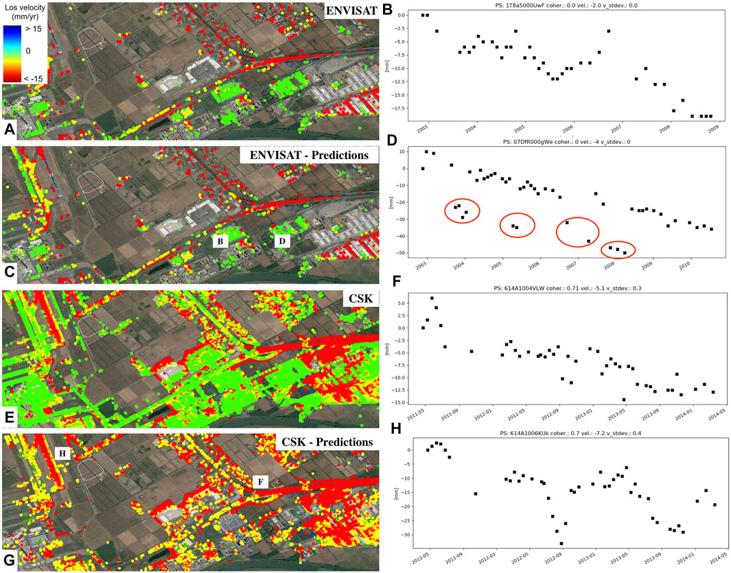
FIGURE 5. Examples of multi-temporal time-series dataset as observed by different sensors: (A) Envisat dataset over the Rome airport. (B) Time series of an anomalous point located over a building moving at –2 mm/year. (C) Envisat dataset Neural Network signals covering the period 2003–2009. Letters B and D represent the location of the time series shown in panels (B) and (D). (D) Anomalous time series moving at an average rate of −4 mm/year. The red circles indicate points in the time series potentially affected by unwrapping errors that in this case have been detected as anomalies. (E) CSK dataset over the Rome airport spanning the period 2011–2014. (F) Time series of an anomalous point located over the highway showing an anomalous behavior between May and July 2011. (G) Time series of anomalous points of the CSK dataset predicted as signals by the neural network approach presented in this paper. Letters F and H represent the location of the time series shown in panels (F) and (H). (H) Time series of displacement related to an area characterized by an anomalous deformation pattern (linear and seasonal) near the airport runaway. Further details on the displacement fields characterizing this area can be found in Bianchini Ciampoli et al. (2020).
Conclusion and Perspectives
We have illustrated the results of a set of experiments based on neural network and pattern recognition techniques toward the creation of a full-automated low-latency system capable of detecting “anomalies” in InSAR time series of surface deformation. The proposed NN system optimizes speed, accuracy (0.9951), and recall (0.9705) compared to the RF. In terms of processing speed, the NN method would process full ERS, ENVISAT, and CSK MapItaly datasets (170MLN time series) in 68 s whereas the RF5 would take 2.2 min. As a comparison, the slowest algorithm (RF500 with engineered features) would take 2.8 h in order to process the entire dataset without considering the processing time spent for calculating the engineered features. Decreasing processing time for large-scale monitoring can be fundamental for mitigating risk and provide warnings within a reasonable time frame given the large amount of SAR data available and the increasing number of SAR sensors that are expected be operational in the near feature. Nonetheless, the proposed experiments presented in this paper can be considered an initial proof of concept of a preliminary early warning system capable of detecting anomalous points in InSAR time series of surface displacement. In the rest of this section, we provide further insights into drawbacks, limitations, and perspectives of the proposed InSAR-based fully automated warning system. One of the most important aspects to consider when considering an InSAR-based detection system is the limitations intrinsic to the InSAR technique itself.
A single time series of surface displacement does not provide a full three-dimensional displacement model; hence, there can be a certain percentage of points on the ground moving toward a direction that the sensor is insensitive to. These points would still be measurable by the sensor and would be classified as true negative whereas deformation is still ongoing toward a direction perpendicular to the LOS. These false negatives would be additional points that not even the analytic algorithm adopted in literature and presented in Anomaly Detection Using an Analytical Model could detect. Di Martire et al. (2017) used the same CSK dataset used in this study and showed that there is a full coincidence between remotely sensed landslide and in situ detected landslide only for 8.07% of in situ landslides, whereas 35.95% of the time, a partial coincidence was found (i.e., the landslide was not fully covered by PS measurements); 44.91% of the dataset showed no coincidence between remotely sensed landslides and in situ landslide monitoring due to lack of coverage or landslide motion perpendicular to the satellite LOS. It should also be pointed out that 11.03% of the SAR dataset showed the presence of new landslides not detected by in situ measurements. The dataset spatial coverage characteristics can be divided into two different satellite subset features: point density and temporal coherence. Point density depends on the satellite spatial resolution, which, in turn, depends on the satellite wavelength (and antenna hardware constrains). Literature studies (Sansosti et al., 2014; Milillo et al., 2015) indicate that an improvement of the coherent pixel density over urban areas (i.e., not affected by temporal decorrelation) achieved by exploiting the high-resolution X-band of the CSK SAR data results in an improvement of point measurement density of 320% and 550% with respect to RADARSAT-1 and ENVISAT data. Point density also depends on the temporal coherence, which, in turn, depends on the radar wavelength and the sampling repeat time. The sampling frequency of a satellite constellation plays a fundamental role in the detection of anomalous time series. A denser acquisition rate is conducive to an increased sensitivity of displacement acceleration and failure time forecast accuracy (Moretto et al., 2017). A recent observational simulation experiment run by Moretto et al. (2017) used ground-based dataset of landslide failures acquired with sub-daily sampling frequency to assess the percentage of predicted landslide failures by under-sampling the sub-daily data to different satellite repeat frequencies. The results showed that given the actual constellations in orbit, only COSMO-SkyMed was able to detect 47 landslides and predict 17 failures within a 5-day error (39% accuracy) whereas the Sentinel constellation accurately predicted only seven failures over 30 landslides detected (23% accuracy). While using the proposed NN approach and supposing the landslide failures are evenly distributed among the satellite full, partial, and null coincidences and considering a total of 100 landslide failures, only 21.5 and 12.7 collapses would be correctly forecasted using the CSK and Sentinel system, respectively, within 5 days of the failure, leading to an NN accuracy of 0.214 and 0.123 for CSK and Sentinel, respectively. These physical constraints are imposed only by satellite data availability, LOS geometry acquisition, and satellite acquisition frequency. Another major constrain is represented by the InSAR time-series processing time itself. As stated in Costantini et al. (2017), the Map-Italy project CSK data time series (time series spanning from 2011 to 2014) took 2 years to process, which is incompatible with a near-real-time processing system. State-of-the-art challenges in the field of InSAR time-series processing are as follows: (1) the need of a time-series processor that does not need to re-process the entire stack when a new image needs to be added to the stack and (2) achieving large-scale cloud processing capabilities over wide areas. Several attempts have been reported in literature presenting state-of-the-art cloud-based InSAR processing systems (Zinno et al., 2015 and 2018; Ferretti et al., 2015; De Luca et al., 2015; Hua et al., 2016), but current cost-effective time-series processing update times lie within 3–6 months on a continental scale (Raspini et al., 2018; Zinno et al., 2018). The proposed NN approach does not take into consideration predisposing and triggering factors such as land cover, terrain geomorphology, DEM slope, and aspect; hence, the predicted anomalous points can also be located in urban areas. A closer analysis of the results (Figures 3, 5) reveals that the anomalous points localized in no-landslide areas correspond to infrastructures showing signs of structural distress or physical phenomena corresponding to increased oil field extraction, aquifer use or volcanic activity (Stramondo et al., 2007; Milillo et al., 2016; Chaussard et al., 2017; Salzer et al., 2017, Macchiarulo et al., 2021). Discriminating and linking time series of surface deformation to the specific physical phenomena causing an acceleration in the time series of displacement would require a more complex network that could take into consideration the aforementioned factors. A starting point for future studies would be the development of a convolutional neural network capable of analyzing spatial features depending on the physical phenomena requested by the user needs (Ermini et al., 2005).
In this paper, we investigate the performances of neural network pattern recognition algorithm toward the creation of a full-automatic anomalies detection system using InSAR time series of surface deformation. Our results indicate that the proposed approach would make the anomaly identification post-processing times negligible when compared to the InSAR time-series processing. Through our experiments, we show how the proposed NN system can provide an accurate and temporally feasible solution reducing the anomalous time-series detection processing times by a factor of 2–147 compared to RF methods and analytical models. Once the existing bottlenecks related to InSAR time-series processing and low satellite data acquisition frequency have been overcome within the next 10 years (Rosen et al., 2019), the proposed approach could be considered a viable solution to a near-real-time fully automatic system for detecting anomalies in InSAR time series of surface deformation.
Data Availability Statement
The original contributions presented in the study are included in the article/Supplementary Material. Further inquiries can be directed to the corresponding author.
Author Contributions
PM wrote the paper and set up the methodology. GS wrote the code for the neural network analysis. HH helped PM write the paper. DM provided access to the historical dataset and participated to time-series analysis data interpretation.
Conflict of Interest
The authors declare that the research was conducted in the absence of any commercial or financial relationships that could be construed as a potential conflict of interest.
Publisher’s Note
All claims expressed in this article are solely those of the authors and do not necessarily represent those of their affiliated organizations, or those of the publisher, the editors, and the reviewers. Any product that may be evaluated in this article, or claim that may be made by its manufacturer, is not guaranteed or endorsed by the publisher.
Acknowledgments
The research was carried out at the Jet Propulsion Laboratory, California Institute of Technology, under a contract with the National Aeronautics and Space Administration. InSAR time-series analysis have been provided by the Italian Ministry of the Environment through the Geoportale Nazionale database (http://www.pcn.minambiente.it/mattm/).
References
Anantrasirichai, N., Biggs, J., Albino, F., and Bull, D. (2019). The Application of Convolutional Neural Networks to Detect Slow, Sustained Deformation in InSAR Timeseries. Geophys. Res. Lett. doi:10.1029/2019gl084993
Berti, M., Corsini, A., Franceschini, S., and Iannacone, J. P. (2013). Automated Classification of Persistent Scatterers Interferometry Time Series. Nat. Hazards Earth Syst. Sci. 13, 1945–1958. doi:10.5194/nhess-13-1945-2013
Bianchini Ciampoli, L., Gagliardi, V., Ferrante, C., Calvi, A., D’Amico, F., and Tosti, F. (2020). Displacement Monitoring in Airport Runways by Persistent Scatterers SAR Interferometry. Remote Sensing 12 (21), 3564. doi:10.3390/rs12213564
Bonì, R., Bosino, A., Meisina, C., Novellino, A., Bateson, L., and McCormack, H. (2018). A Methodology to Detect and Characterize Uplift Phenomena in Urban Areas Using Sentinel-1 Data. Remote Sensing 10, 607. doi:10.3390/rs10040607
Bonì, R., Meisina, C., Poggio, L., Fontana, A., Tessari, G., Riccardi, P., et al. (2020). Ground Motion Areas Detection (GMA-D): an Innovative Approach to Identify Ground Deformation Areas Using the SAR-Based Displacement Time Series. Proc. IAHS 382, 277–284. doi:10.5194/piahs-382-277-2020
Bonì, R., Pilla, G., and Meisina, C. (2016). Methodology for Detection and Interpretation of Ground Motion Areas with the A-DInSAR Time Series Analysis. Remote Sensing 8 (8), 686. doi:10.3390/rs8080686
Burrows, K., Walters, R. J., Milledge, D., Spaans, K., and Densmore, A. L. (2019). A New Method for Large-Scale Landslide Classification from Satellite Radar. Remote Sensing 11 (3), 237. doi:10.3390/rs11030237
Carlà, T., Intrieri, E., Raspini, F., Bardi, F., Farina, P., Ferretti, A., et al. (2019). Perspectives on the Prediction of Catastrophic Slope Failures from Satellite InSAR. Sci. Rep. 9 (1), 14137–14139. doi:10.1038/s41598-019-50792-y
Chang, L., and Hanssen, R. F. (2016). A Probabilistic Approach for InSAR Time-Series Postprocessing. IEEE Trans. Geosci. Remote Sensing 54, 421–430. doi:10.1109/tgrs.2015.2459037
Chaussard, E., Milillo, P., Bürgmann, R., Perissin, D., Fielding, E. J., and Baker, B. (2017). Remote Sensing of Ground Deformation for Monitoring Groundwater Management Practices: Application to the Santa Clara Valley during the 2012-2015 California Drought. J. Geophys. Res. Solid Earth 122 (10), 8566–8582. doi:10.1002/2017jb014676
Cheriyadat, A. M. (2014). Unsupervised Feature Learning for Aerial Scene Classification. IEEE Trans. Geosci. Remote Sensing 52 (1), 439–451. doi:10.1109/tgrs.2013.2241444
Cigna, F., Del Ventisette, C., Liguori, V., and Casagli, N. (2011). Advanced Radar-Interpretation of InSAR Time Series for Mapping and Characterization of Geological Processes. Nat. Hazards Earth Syst. Sci. 11 (3), 865–881. doi:10.5194/nhess-11-865-2011
Confuorto, P., Di Martire, D., Centolanza, G., Iglesias, R., Mallorqui, J. J., Novellino, A., et al. (2017). Post-failure Evolution Analysis of a Rainfall-Triggered Landslide by Multi-Temporal Interferometry SAR Approaches Integrated with Geotechnical Analysis. Remote Sensing Environ. 188, 51–72. doi:10.1016/j.rse.2016.11.002
Costantini, M., Ferretti, A., Minati, F., Falco, S., Trillo, F., Colombo, D., et al. (2017). Analysis of Surface Deformations over the Whole Italian Territory by Interferometric Processing of ERS, Envisat and COSMO-SkyMed Radar Data. Remote Sensing Environ. 202, 250–275. doi:10.1016/j.rse.2017.07.017
De Luca, C., Cuccu, R., Elefante, S., Zinno, I., Manunta, M., Casola, V., et al. (2015). An On-Demand Web Tool for the Unsupervised Retrieval of Earth's Surface Deformation from SAR Data: The P-SBAS Service within the ESA G-POD Environment. Remote Sensing 7 (11), 15630–15650. doi:10.3390/rs71115630
Di Martire, D., Paci, M., Confuorto, P., Costabile, S., Guastaferro, F., Verta, A., et al. (2017). A Nation-wide System for Landslide Mapping and Risk Management in Italy: The Second Not-ordinary Plan of Environmental Remote Sensing. Int. J. Appl. earth observation geoinformation 63, 143–157. doi:10.1016/j.jag.2017.07.018
Ermini, L., Catani, F., and Casagli, N. (2005). Artificial Neural Networks Applied to Landslide Susceptibility Assessment. Geomorphology 66 (1-4), 327–343. doi:10.1016/j.geomorph.2004.09.025
Ferretti, A., Colombo, D., Fumagalli, A., Novali, F., and Rucci, A. (2015). InSAR Data for Monitoring Land Subsidence: Time to Think Big. Proc. IAHS 372, 331–334. doi:10.5194/piahs-372-331-2015
Fiorentini, N., Maboudi, M., Losa, M., and Gerke, M. (2020). Assessing Resilience of Infrastructures towards Exogenous Events by Using PS-InSAR-Based Surface Motion Estimates and Machine Learning Regression Techniques. ISPRS Ann. Photogramm. Remote Sens. Spat. Inf. Sci. V-4-2020, 19–26. doi:10.5194/isprs-annals-v-4-2020-19-2020
Gaddes, M. E., Hooper, A., and Bagnardi, M. (2019). Using Machine Learning to Automatically Detect Volcanic Unrest in a Time Series of Interferograms. J. Geophys. Res. Solid Earth. doi:10.1029/2019jb017519
Giardina, G., Milillo, P., DeJong, M. J., Perissin, D., and Milillo, G. (2019). Evaluation of InSAR Monitoring Data for post‐tunnelling Settlement Damage Assessment. Struct. Control. Health Monit. 26 (2), e2285. doi:10.1002/stc.2285
Hinton, G. E., Srivastava, N., Krizhevsky, A., Sutskever, I., and Salakhutdinov, R. R. (2012). Improving Neural Networks by Preventing Co-adaptation of Feature Detectors. arXiv preprint arXiv:1207.0580.
Hua, H., Rosen, P., Owen, S., Manipon, G., Starch, M., Dang, L., et al. (2016). SAR Science Data Processing (SDP) Foundry.
Infante, D., Di Martire, D., Confuorto, P., Tessitore, S., Tòmas, R., Calcaterra, D., et al. (2019). Assessment of Building Behavior in Slow-Moving Landslide-Affected Areas through DInSAR Data and Structural Analysis. Eng. Structures 199, 109638. doi:10.1016/j.engstruct.2019.109638
Intrieri, E., Raspini, F., Fumagalli, A., Lu, P., Del Conte, S., Farina, P., et al. (2018). The Maoxian Landslide as Seen from Space: Detecting Precursors of Failure with Sentinel-1 Data. Landslides 15 (1), 123–133. doi:10.1007/s10346-017-0915-7
Ioffe, S., and Szegedy, C. (2015). Batch Normalization: Accelerating Deep Network Training by Reducing Internal Covariate Shift. arXiv preprint arXiv:1502.03167.
Ito, Y., Hosokawa, M., Lee, H., and Liu, J. G. (2000). Extraction of Damaged Regions Using SAR Data and Neural Networks. Int. Arch. Photogrammetry Remote Sensing 33 (B1), 156–163. PART 1.
Ji, M., Liu, L., Du, R., and Buchroithner, M. F. (2019). A Comparative Study of Texture and Convolutional Neural Network Features for Detecting Collapsed Buildings after Earthquakes Using Pre- and Post-Event Satellite Imagery. Remote Sensing 11 (10), 1202. doi:10.3390/rs11101202
Karimzadeh, S., and Matsuoka, M. (2018). A Weighted Overlay Method for Liquefaction-Related Urban Damage Detection: A Case Study of the 6 September 2018 Hokkaido Eastern Iburi Earthquake, Japan. Geosciences 8, 487. doi:10.3390/geosciences8120487
Kelevitz, K., Tiampo, K. F., and Corsa, B. D. (2021). Improved Real-Time Natural Hazard Monitoring Using Automated DInSAR Time Series. Remote Sensing 13 (5), 867. doi:10.3390/rs13050867
Lazebnik, S., Schmid, C., and Ponce, J. (2006). Beyond Bags of Features: Spatial Pyramid Matching Forrecognizing Natural Scene Categories. in Proc. IEEE Comp. Soc. Conf. Comp. Vis. Pattern Recognition 2, 2169–2178.
Macchiarulo, V., Milillo, P., Blenkinsopp, C., and Giardina, G. (2021). Monitoring Deformations of Infrastructure Networks: A Fully Automated GIS Integration and Analysis of InSAR Time-Series. In Structural Health Monitoring. doi:10.1177/14759217211045912
Macchiarulo, V., Milillo, P., DeJong, M. J., González Martí, J., Sánchez, J., and Giardina, G. (2021). Integrated InSAR Monitoring and Structural Assessment of Tunnelling‐induced Building Deformations. Structural Control and Health Monitoring, e2781.
Maskey, M., Ramachandran, R., and Miller, J. (2017). Deep Learning for Phenomena-Based Classification of Earth Science Images. J. Appl. Remote Sens 11 (4), 1. doi:10.1117/1.JRS.11.042608
Meisina, C., Zucca, F., Notti, D., Colombo, A., Cucchi, A., Savio, G., et al. (2008). Geological Interpretation of PSInSAR Data at Regional Scale. Sensors 8 (11), 7469–7492. doi:10.3390/s8117469
Milillo, P., Bürgmann, R., Lundgren, P., Salzer, J., Perissin, D., Fielding, E., et al. (2016). Space Geodetic Monitoring of Engineered Structures: The Ongoing Destabilization of the Mosul Dam, Iraq. Sci. Rep. 6, 37408. doi:10.1038/srep37408
Milillo, P., Giardina, G., DeJong, M., Perissin, D., and Milillo, G. (2018). Multi-temporal InSAR Structural Damage Assessment: The London Crossrail Case Study. Remote Sensing 10 (2), 287. doi:10.3390/rs10020287
Milillo, P., Giardina, G., Perissin, D., Milillo, G., Coletta, A., and Terranova, C. (2019). Pre-Collapse Space Geodetic Observations of Critical Infrastructure: The Morandi Bridge, Genoa, Italy. Remote Sensing 11 (12), 1403. doi:10.3390/rs11121403
Milillo, P., Riel, B., Minchew, B., Yun, S. H., Simons, M., and Lundgren, P. (2015). On the Synergistic Use of SAR Constellations’ Data Exploitation for Earth Science and Natural hazard Response. IEEE J. Selected Top. Appl. Earth Observations Remote Sensing 9 (3), 1095–1100.
Milone, G., and Scepi, G. (2011). A Clustering Approach for Studying Ground Deformation Trends in Campania Region through PS-InSARTM Time Series Analysis. J. Appl. Sci. 11, 610–620. doi:10.3923/jas.2011.610.620
Moretto, S., Bozzano, F., Esposito, C., Mazzanti, P., and Rocca, A. (2017). Assessment of Landslide Pre-failure Monitoring and Forecasting Using Satellite SAR Interferometry. Geosciences 7 (2), 36. doi:10.3390/geosciences7020036
Ngo, P.-T., Hoang, N.-D., Pradhan, B., Nguyen, Q., Tran, X., Nguyen, Q., et al. (2018). A Novel Hybrid Swarm Optimized Multilayer Neural Network for Spatial Prediction of Flash Floods in Tropical Areas Using Sentinel-1 SAR Imagery and Geospatial Data. Sensors 18 (11), 3704. doi:10.3390/s18113704
Notti, D., Calò, F., Cigna, F., Manunta, M., Herrera, G., Berti, M., Meisina, C., Tapete, D., and Zucca, F. (2015). A User-Oriented Methodology for DInSAR Time Series Analysis and Interpretation: Landslides and Subsidence Case Studies. Pure Appl. Geophys. 172 (11), 3081–3105. doi:10.1007/s00024-015-1071-4
Pedregosa, F., Varoquaux, G., Gramfort, A., Michel, V., Thirion, B., Grisel, O., et al. (2011). Scikit-learn: Machine Learning in Python. J. machine Learn. Res. 12, 2825–2830.
Penatti, B., Nogueira, K., and Santos, J. A., Do deep Features Generalize from Everyday Objects to Remote Sensing and Aerial Scenes Domains in IEEE Conf. on Computer Vision and Pattern Recognition Workshops (CVPRW ’15). 44–51 (2015).
Pratesi, F., Tapete, D., Terenzi, G., Del Ventisette, C., and Moretti, S. (2015). Rating Health and Stability of Engineering Structures via Classification Indexes of InSAR Persistent Scatterers. Int. J. Appl. earth observation geoinformation 40, 81–90. doi:10.1016/j.jag.2015.04.012
Raspini, F., Bianchini, S., Ciampalini, A., Del Soldato, M., Solari, L., Novali, F., et al. (2018). Continuous, Semi-automatic Monitoring of Ground Deformation Using Sentinel-1 Satellites. Sci. Rep. 8 (1), 7253. doi:10.1038/s41598-018-25369-w
Refice, A., Capolongo, D., Pasquariello, G., DaAddabbo, A., Bovenga, F., Nutricato, R., et al. (2014). SAR and InSAR for Flood Monitoring: Examples with COSMO-SkyMed Data. IEEE J. Sel. Top. Appl. Earth Observations Remote Sensing 7 (7), 2711–2722. doi:10.1109/jstars.2014.2305165
Reinosch, E., Gerke, M., Riedel, B., Schwalb, A., Ye, Q., and Buckel, J. (2021). Rock Glacier Inventory of the Western Nyainqêntanglha Range, Tibetan Plateau, Supported by InSAR Time Series and Automated Classification. In Permafrost and Periglacial Processes.
Rosen, P. A., Horst, S. J., Khazendar, A., Milillo, P., Oveisgharan, S., Owen, S. E., et al. (2019).NASA’s Next Generation Surface Deformation and Change Observing System Architecture. In IGARSS 2019-2019 IEEE International Geoscience and Remote Sensing Symposium. IEEE, 8378–8380. doi:10.1109/igarss.2019.8899231
Salzer, J. T., Milillo, P., Varley, N., Perissin, D., Pantaleo, M., and Walter, T. R. (2017). Evaluating links between deformation, topography and surface temperature at volcanic domes: Results from a multi-sensor study at Volcán de Colima, Mexico. Earth Planet. Sci. Lett. 479, 354–365. doi:10.1016/j.epsl.2017.09.027
Sansosti, E., Berardino, P., Bonano, M., Calò, F., Castaldo, R., Casu, F., et al. (2014). How Second Generation SAR Systems Are Impacting the Analysis of Ground Deformation. Int. J. Appl. Earth Observation Geoinformation 28, 1–11. doi:10.1016/j.jag.2013.10.007
Schmidhuber, J. (2015). Deep Learning in Neural Networks: An Overview. Neural networks 61, 85–117. doi:10.1016/j.neunet.2014.09.003
Selvakumaran, S., Plank, S., Geiß, C., Rossi, C., and Middleton, C. (2018). Remote Monitoring to Predict Bridge Scour Failure Using Interferometric Synthetic Aperture Radar (InSAR) Stacking Techniques. Int. J. Appl. Earth Observation Geoinformation 73, 463–470. doi:10.1016/j.jag.2018.07.004
Sica, F., Gobbi, G., Rizzoli, P., and Bruzzone, L. (2020). Φ-Net: Deep Residual Learning for InSAR Parameters Estimation. IEEE Trans. Geosci. Remote Sensing 59 (5), 3917–3941.
Sousa, J. J., and Bastos, L. (2013). Multi-temporal SAR Interferometry Reveals Acceleration of Bridge Sinking before Collapse. Nat. Hazards Earth Syst. Sci. 13, 659–667. doi:10.5194/nhess-13-659-2013
Stramondo, S., Saroli, M., Tolomei, C., Moro, M., Doumaz, F., Pesci, A., et al. (2007). Surface Movements in Bologna (Po Plain - Italy) Detected by Multitemporal DInSAR. Remote Sensing Environ. 110 (3), 304–316. doi:10.1016/j.rse.2007.02.023
Tomás, R., Pagán, J. I., Navarro, J. A., Cano, M., Pastor, J. L., Riquelme, A., Cuevas-González, J. M., Crosetto, fnm., Barra, fnm., Monserrat, fnm., Lopez-Sanchez, fnm., Ramón, fnm., Ivorra, fnm., Soldato, fnm., Solari, fnm., Bianchini, fnm., Raspini, fnm., Novali, fnm., Ferretti, fnm., Costantini, fnm., Trillo, fnm., Herrera, fnm., and Casagli, fnm. (2019). Semi-Automatic Identification and Pre-screening of Geological-Geotechnical Deformational Processes Using Persistent Scatterer Interferometry Datasets. Remote Sensing 11 (14), 1675. doi:10.3390/rs11141675
Trigila, A., and Iadanza, C. (2018). Landslides and Floods in Italy: hazard and Risk Indicators - Summary Report 2018. doi:10.13140/RG.2.2.14114.48328
Valade, S., Ley, A., Massimetti, F., D’Hondt, O., Laiolo, M., Coppola, D., et al. (2019). Towards Global Volcano Monitoring Using Multisensor Sentinel Missions and Artificial Intelligence: The MOUNTS Monitoring System. Remote Sensing 11 (13), 1528. doi:10.3390/rs11131528
Yun, S.-H., Hudnut, K., Owen, S., Webb, F., Simons, M., Sacco, P., et al. (2015). Rapid Damage Mapping for the 2015Mw 7.8 Gorkha Earthquake Using Synthetic Aperture Radar Data from COSMO-SkyMed and ALOS-2 Satellites. Seismological Res. Lett. 86 (6), 1549–1556. doi:10.1785/0220150152
Zhao, Z., Wu, Z., Zheng, Y., and Ma, P. (2021). Recurrent Neural Networks for Atmospheric Noise Removal from InSAR Time Series with Missing Values. ISPRS J. Photogrammetry Remote Sensing 180, 227–237. doi:10.1016/j.isprsjprs.2021.08.009
Zinno, I., Bonano, M., Buonanno, S., Casu, F., De Luca, C., Manunta, M., et al. (2018). National Scale Surface Deformation Time Series Generation through Advanced DInSAR Processing of Sentinel-1 Data within a Cloud Computing Environment. IEEE Trans. Big Data.
Keywords: multi-temporal InSAR, anomalies detection, landslides, infrastructure monitoring, pattern recognition, neural network, surface displacement, geodetic measurements
Citation: Milillo P, Sacco G, Di Martire D and Hua H (2022) Neural Network Pattern Recognition Experiments Toward a Fully Automatic Detection of Anomalies in InSAR Time Series of Surface Deformation. Front. Earth Sci. 9:728643. doi: 10.3389/feart.2021.728643
Received: 21 June 2021; Accepted: 08 November 2021;
Published: 01 February 2022.
Edited by:
Antonio Pepe, National Research Council (CNR), ItalyReviewed by:
Konstantinos Demertzis, International Hellenic University, GreeceChandrakanta Ojha, Indian Institute of Science Education and Research Mohali, India
Copyright © 2022 Milillo, Sacco, Di Martire and Hua. This is an open-access article distributed under the terms of the Creative Commons Attribution License (CC BY). The use, distribution or reproduction in other forums is permitted, provided the original author(s) and the copyright owner(s) are credited and that the original publication in this journal is cited, in accordance with accepted academic practice. No use, distribution or reproduction is permitted which does not comply with these terms.
*Correspondence: Pietro Milillo, cG1pbGlsbG9AY2VudHJhbC51aC5lZHU=