Ocean Mesoscale Variability: A Case Study on the Mediterranean Sea From a Re-Analysis Perspective

The mesoscale variability in the Mediterranean Sea is investigated through eddy detection techniques. The analysis is performed over 24 years (1993–2016) considering the three-dimensional (3D) fields from an ocean re-analysis of the Mediterranean Sea (MED-REA). The objective is to achieve a fit-for-purpose assessment of the 3D mesoscale eddy field. In particular, we focus on the contribution of eddy-driven anomalies to ocean dynamics and thermodynamics. The accuracy of the method used to disclose the 3D eddy contributions is assessed against pointwise in-situ measurements and observation-based data sets. Eddy lifetimes ≥ 2 weeks are representative of the 3D mesoscale field in the basin, showing a high probability (> 60%) of occurrence in the areas of the main quasi-stationary mesoscale features. The results show a dependence of the eddy size and thickness on polarity and lifetime: anticyclonic eddies (ACE) are significantly deeper than cyclonic eddies (CE), and their size tends to increase in long-lived structures which also show a seasonal variability. Mesoscale eddies result to be a significant contribution to the ocean dynamics in the Mediterranean Sea, as they account for a large portion of the sea-surface height variability at temporal scales longer than 1 month and for the kinetic energy (50–60%) both at the surface and at depth. Looking at the contributions to ocean thermodynamics, the results exhibit the existence of typical warm (cold) cores associated with ACEs (CEs) with exceptions in the Levantine basin (e.g., Shikmona gyre) where a structure close to a mode-water ACE eddy persists with a positive salinity anomaly. In this area, eddy-induced temperature anomalies can be affected by a strong summer stratification in the surface water, displaying an opposite sign of the anomaly whether looking at the surface or at depth. The results show also that temperature anomalies driven by long-lived eddies (≥ 4 weeks) can affect up to 15–25% of the monthly variability of the upper ocean heat content in the Mediterranean basin.

1 Introduction

Mesoscale eddies can originate nearly everywhere in the ocean, and typically exhibit different properties (e.g., heat, salt, carbon) with respect to their surroundings, which can be transported as they move around the ocean (Chelton et al., 2007; Chelton et al., 2011b; Zhao et al., 2018). At the surface, mesoscale eddies are identified from satellite altimetry data, where depression (elevation) in the sea level anomaly (SLA) field reveals a cyclonic (anticyclonic) structure (Chelton et al., 2011a). Although only the surface expression of mesoscale eddies is visible in remote sensing measurement of SLA and sea-surface temperature (SST), they are three-dimensional (3D) structures that can reach down into the pycnocline. Temperature and salinity anomalies induced by eddies tend to be opposite depending on the polarity of an eddy: cyclones (CE) versus anticyclones (ACE) (Gaube et al., 2013; Dong et al., 2014; Raj et al., 2016; Raj et al., 2020). Mode-water eddies represent a substantial exception to this general rule (Barceló-Llull et al., 2017; Zhang et al., 2017; Shi et al., 2018). Schütte et al. (2016) show the existence of ACEs with both negative SST and salinity anomaly and positive ones. Pegliasco et al. (2015) observed ACEs with a lens-like structure of isopycnals in the eastern boundary upwelling regions. In this context, eddy-detection systems (e.g., Dong et al., 2012; Petersen et al., 2013; Xu et al., 2014; Faghmous et al., 2015; Frenger et al., 2015; Lin et al., 2015) are an ad-hoc diagnostic tool designed to isolate mesoscale features, track them in time, and exclusively analyze the parcel of water trapped inside. These systems can disentangle the “anomalous” content dragged by eddies, that can differ from the ambient waters, in terms of nutrient concentration, tracers, and energetic component. Combining multiple observing system networks, from in-situ and remote-sensing, it is now possible to investigate eddy-induced anomalies in water mass structures, estimate ocean heat, and salt transport by advective trapping (e.g. Gaube et al., 2013; Dong et al., 2014), and hence infer the quasi-3D structure of the non-linear features. Conversely, the representation of ocean mesoscale dynamics is strongly limited by the spatial coverage and temporal sampling of a given satellite mission (e.g., Bonaduce et al., 2018; Chen et al., 2021). Moreover, the temporal and spatial co-location with the available Argo profiling floats in certain areas of the ocean is affected by uneven data coverage and sampling frequency (e.g., Liu et al., 2020), which can represent a shortcoming to investigate the properties of water masses induced by the occurrence of 3D eddies.

These limitations can be overcome by exploiting the synergy between multiple observing systems and ocean model dynamics. Ocean re-analyses combine information from multiple observing networks (e.g., satellite altimetry and Argo profiling floats) with ocean model dynamics and atmospheric forcing through multivariate data assimilation methods (Storto et al., 2019) to obtain optimized 4D estimates of the state of the ocean. These are non-linear, dynamically-reconstructed ocean fields that outperform observation-only reconstructed products in several crucial climate indexes (Wunsch and Heimbach, 2014; Balmaseda et al., 2015), as well as in the representation of the small-scale variability at depth (Cipollone et al., 2017).

The objective of this work is to achieve a fit-for-purpose assessment of the representation of the 3D structure of mesoscale eddies in a regional ocean reanalysis for the Mediterranean Sea.

In this area, eddies have a deep and stable structure, penetrating well below the mixed layer depth down to 400–500 m (e.g., Fusco et al., 2003). Their structures are almost stationary, mainly trapped between the most prominent ocean currents of the basin (e.g., Pinardi et al., 1997; Pinardi and Masetti, 2000; Pinardi et al., 2015), thus behaving like a preferred energetic pathway to transform potential into eddy kinetic energy (EKE) and mixing deep and surface water (e.g., Rubio et al., 2009). A mere look at surface physics only would be a too coarse approximation, and it is therefore crucial to have access to the full 3D eddy structure, for any quantitative estimate of anomalous flow and the impact on ocean circulation and water masses. The features of the ocean circulation in the Mediterranean Sea have been investigated so far from either models or observations. A fundamental contribution to the understanding of ocean general circulation and mesoscale dynamics in the Mediterranean Sea was made by the Physical Oceanography of the Eastern Mediterranean Group, based on innovative observational strategy and pioneering numerical simulations (e.g., Robinson et al., 1992; Robinson and Golnaraghi, 1993; Robinson et al., 2001). Comparing the geostrophic velocities derived from satellite altimetry missions (ERS-1 and TOPEX/Poseidon; Ayoub et al., 1998) and ocean currents from numerical experiments, Pinardi and Masetti (2000) emphasized the influence of the eddy field on large scale circulation. Pinardi et al. (2015), considering ocean currents from model re-analyses over 2 decades, achieved a new schematic of ocean circulation in the Mediterranean Sea, and underlined how cyclonic and anticyclonic gyres in the northern and southern parts of the basin, respectively, characterize the large scale circulation. Observations and model-based activities were carried out by Marullo et al. (2003) to investigate the variability of the mixed layer in the Levantine basin driven by the Rhodes and Ierapetra Gyres. Fernandez et al. (2005) studied the interannual eddy-driven variability and showed that it is persistent and evolves slowly, independently of the annual cycle of the atmospheric forcing. The anomalies in the circulation patterns can happen not only in the top layers but also in deeper layers, which are hardly related to the changes in the atmospheric forcing. Escudier et al. (2016) described the 3D structure of the western Mediterranean basin eddies by using several eddy-resolving model simulations and satellite altimetry. Considering a similar spatial domain, Mason et al. (2019) compared global and regional operational models to obtain new insight into the 3D eddy properties. Mkhinini et al. (2014) studied a long-lived eddy in the eastern part of the basin analyzing 2D altimetry maps. Well-known stationary eddies in the Levantine basin were the subject of specific oceanographic campaigns (Ioannou et al., 2017; Mauri et al., 2019; Velaoras et al., 2019).

In this work, we focus on the Mediterranean basin to investigate the entire 3D mesoscale field that emerges from an eddy-resolving ocean re-analysis. In particular, we look at the surface and 3D signatures of the non-linear eddy structures and their contributions to the kinetic energy in the ocean and the vertical structure of water masses. The consolidated ocean re-analysis considered in this work (Simoncelli et al., 2019) is implemented in the region at a horizontal resolution of 1/16° (Oddo et al., 2014; Tonani et al., 2015) which provides an excellent playground in terms of resolution and eddy population.

The renalysis dataset explored covers 24 years (1993–2016) of daily averaged fields with a grid spacing of about 6–7 km (the exact spacing varies according to latitude). Although sub-mesoscale processes, not presently included in the circulation model, are known to have an impact on mesoscale fronts and vortexes (Haza et al., 2012; Sasaki et al., 2014), this resolution is sufficient to sustain turbulence generated by the model itself at the first baroclinic wavelength or coming from assimilation procedure increments. In this sense, the Mediterranean region is fully resolved both at spatial (Hallberg, 2013) and temporal scale, i.e., eddies can be followed in time with daily sub-sampling while their typical lifetime ranges between several days and few months.

The paper is organized as follows: Section 2 describes the ocean re-analysis and eddy detection algorithm considered to characterize the 3D mesoscale structures in the Mediterranean Sea. Section 3 assesses the accuracy of the methodology by comparing with observations and describes the eddy contributions to ocean dynamics and water masses structure (thermodynamics). Section 4 summarizes and provides conclusions to this work.

2 Materials and Methods

2.1 Mediterranean Re-Analysis

The version of MED-REA used in this work (Simoncelli et al., 2019) relies on a fully eddy-resolving horizontal resolution (6–7 km) ocean general circulation model (OGCM), based on the Nucleus for European Modelling of the Ocean (NEMO; Madec, 2016) and implemented in the Mediterranean region (Oddo et al., 2009; Oddo et al., 2014). The system is extensively validated against in-situ and remote-sensing observations and, up to 2020 provided also operational services within the framework of the Copernicus Marine Environment and Monitoring Service (CMEMS). The MED-REA is forced by the 6-h, 0.75° horizontal-resolution Era-Interim atmospheric re-analysis (Dee et al., 2011) from the European Center for Medium-Range Weather Forecast (ECMWF) and global ocean monthly mean climatology fields (Drévillon et al., 2008) are considered as lateral open boundary conditions (Oddo et al., 2009). The assimilative system considers the most updated and best quality flagged observational records of temperature (T), salinity (S), and sea surface height (SSH), retrieved from a variety of observational networks (both from in-situ and remote-sensing observations), which are ingested into the system during the numerical integration, through a 3D variational (3D-VAR; Dobricic and Pinardi, 2008) data assimilation scheme, to obtain an ocean synthesis which has the potential to provide more accurate information than observation-only or model-only based ocean estimations (e.g., Heimbach et al., 2019). We explore MED-REA daily outputs of SSH, zonal and meridional currents, ocean temperature, and salinity over a 24-year period (1993–2016) to investigate the mesoscale eddies in the Mediterranean region, through innovative eddy detection and tracking methods.

2.2 Methods

In this Section, we exploit a three-dimensional eddy-detection system (Cipollone et al., 2017) capable of constraining 3D mesoscale structures simultaneously through static and dynamic features (see Supplementary Appendix SA). The system has been improved to extract the “anomalous” eddy content in contrast to its non-homogeneous surrounding water. Eddy and background values are extracted at the same time thus removing any potential bias coming from calculations based on climatological fields or spatial smoothing. The accuracy of the method is assessed against in-situ observations in one specific region of the Mediterranean Sea (MED) where a number of Argo profiling floats (Good et al., 2013) are present both within and outside of the eddy (∼500 floats during the period 2008–2010).

The background to the observed eddy-driven anomalies are defined in the temperature and salinity fields. We consider eddy-specific temporal and spatial scales to define the properties of the surrounding water masses, which are then considered as a reference for estimates of the anomalies induced by the mesoscale 3D features. A detailed description of the eddy detection and tracking algorithm is given in Supplementary Appendix SA.

2.2.1 Definition of Spatial Anomaly in Presence of Non-Homogeneous Background

The notion of “anomaly” generally refers to a certain phenomenon or signal that departs from a “standard” background field and brings therefore a non-zero information content (e.g., Wilks, 2011). While the anomalous behaviour is simple to detect by inspection qualitatively, on the other hand, it is not always obvious how to more quantitatively define what should be retained in the background and what should contribute to the anomaly. In oceanography, climatological fields are often used as a proxy for the identification of “standard” behaviours. The time average is therefore used as a spatial smoother and therefore the main stationary, cyclical phenomena are retained in the background term, i.e., the total field Q may be expressed as:

$\begin{array}{ccc}\hfill & Q(t,x,y)=\hfill & \bar{Q}{(\mathrm{mod}(t,\mathrm{\Delta }t),x,y)}_{\text{clim}}+Q_{\text{anom}}(t,x,y)\mathrm{w}\mathrm{h}\mathrm{e}\mathrm{r}\mathrm{e}\hfill \\ \hfill & \bar{Q}(i,x,y)=\hfill & \frac{1}{N}\sum _{j=1}^{N}Q(j\mathrm{*}\mathrm{\Delta }\mathit{t}+\mathit{i},\mathit{x},\mathit{y})\mathrm{w}\mathrm{i}\mathrm{t}\mathrm{h}i\in [1,\mathrm{\Delta }t]N=\mathrm{i}\mathrm{n}\mathrm{t}[dim(t)/\mathrm{\Delta }t]\hfill \end{array}(1)$

where Δt represents the length of the temporal cycle (typically 1 year), $\bar{Q}$ is the background stationary part, and Q_anom is the turbulent component containing the anomalous signal to extract. In the context of mesoscale variability, Eq. 1 can be considered a first-order approximation that suffers the possible presence of trends and strong bias due to the fact that the climatological background can be far from the actual background for a specific year. In Mason et al. (2019) and Gaube et al. (2014) a spatial Gaussian smoother with a half width of 6° is used to remove the mesoscale variability and define the background. In the following, we employ a bias-free method where the anomaly is calculated with respect to the local “surrounding” waters at the eddy perimeter (Figures 1A–F). The calculation of anomaly is based on the creation of a background field that mimics a continuous tracer field in the absence of eddy, by replacing it with “surrounding” waters. However, these “surrounding” waters can be not as homogeneous as expected. In an area of strong density gradient or close to the coast, it is not unusual for an eddy to have a heterogeneous perimeter, with opposite sides floating in water that can differ by several degrees. In this case, the choice of the “surrounding” water cannot be a unique value, the use of the mean of the perimetral annulus could generate a background value that is, discontinuous at the eddy border and largely depending on the exact location and extension of the perimeter. Such a perimeter can change during time, extending more in the cold/warm part of the region, thus changing substantially the reference mean. In the current methodology, to avoid any artifacts coming from the definition of “surrounding” waters, each inner point of the eddy is filled with values “extrapolated” from the closest perimetrical points (Figure 1). The inner (eddy) annulus closest to the eddy perimeter is filled first, each point is replaced with the mean value of the closest ocean points (up to four points) from the eddy perimeter. When the first inner annulus is filled, the algorithm proceeds with the second inner annulus till the eddy center. The background obtained in this case does not have any discontinuity at the eddy perimeter. The spatial structure of the anomaly is rather robust depending on the local boundary values avoiding possible non-local effects coming from temperature values that differ at the other side of the eddy.

FIGURE 1

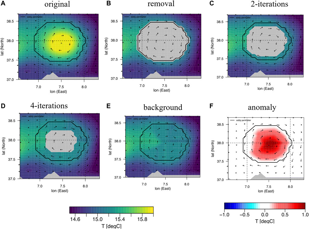
FIGURE 1. Calculation of the eddy anomaly: (A) original temperature field with an eddy detected and delimited by its perimeter (black line). Vectors correspond to ocean currents. (B) The parcel of water delimited by the perimeter is masked. (C) and (D) Temperature values outside the perimeter are extrapolated inside the mask (see Section 2) to define the background field (E). 4) The anomaly (F) is finally obtained as the difference between the original tracer field and the background.

The overall procedure is shown in Figure 1: once the eddy is detected (a), the algorithm removes the corresponding area in the tracer field (b), and extrapolates the border values to fill the missing area (c and d) thus generating a possible background field (e). The anomaly (f) is then calculated with respect to such field as follows:

$Q_{\text{anom}}(t,x,y)=Q(t,x,y)-{⟨Q⟩}_{\text{back}}(t,x,y)(2)$

where the interpolation starts from the eddy contour using the closest ocean points out of the eddy, and proceeds inside to obtain a background guess ⟨Q⟩_back (t, x, y). The method reduces to a minimum the inclusion of spurious biases coming from a sub-optimal definition of the background field and the impact of seasonal variability. A second benefit is that the overall results are pretty stable as a function of the eddy lifetime. The inclusion of spurious eddies would lead to an underestimation of the eddy anomaly content, being inner and outer water similar and the spatial anomaly close to zero. Another source of underestimation can come from the fact that the detected perimetral water partially overlaps with the anomaly itself (Figure 1). In the following Section, the method is applied in a case study and compared with observations to assess the overall skill.

3 Results

In this Section we first validate the eddy-detection method used to investigate eddy-driven three-dimensional anomalies, looking at a specific case study in the Levantine basin, which is the area of the Mediterranean Sea characterized by prominent mesoscale features of the ocean circulation (e.g., Alhammoud et al., 2005). We then continue describing the 3D mesoscale field that emerges from the analysis of eddy-driven content in Mediterranean re-analysis.

3.1 A Case Study: The Shikmona Gyre Area

The sparsity of profiling data usually prevents an instantaneous and direct measure of the 3D eddy anomaly content. Such a measure requires the sampling of at least two different profiling floats at the same time; one trapped inside the eddy while the other acts as a probe mapping the surroundings. Thanks to the recent deployment of the array of Argo profiling floats an increasing number of such dual observations are becoming freely available. We select an area in the Levantine basin well documented by several different types of observations and for which there can be found some long-lasting measurements of two or more profilers with one profiler effectively trapped by the quasi-stationary structure that usually occurs in that area. These data are taken from the Met Office EN4 dataset that gathers quality-controlled subsurface ocean temperature and salinity profiles (v4.2.1; Good et al., 2013). The area is delimited by the green box shown in Figure 2A and corresponds to the area where a quasi-stationary mode-water ACE generally occurs. This eddy has recently been well documented by two cruises in Mauri et al., 2019 that show the peculiar characteristics with saltier and warmer temperature at depth. The measure of the temperature anomaly profile from observations is calculated only when two or more profilers occur within the target area on the same day, with one float trapped within the eddy. The identification of trapped observations usually relies on the analysis of altimetry maps, reconstructed from along-track satellite retrievals (Dong et al., 2014; Zhang et al., 2016), which entails an eddy-detection performed on a two-dimensional SLA field. Floats are considered trapped if they profile inside the SLA-eddy pattern. In our study, on the other hand, a profile is considered trapped if it occurs inside the 3D eddy structure detected from the MED-REA. The use of a 3D ocean re-analysis allows assessment of whether the eddy anomaly estimated in the model (T_eddy − T_back), is also measured by the profilers ($T_{eddy}^{obs}-T_{back}^{obs}$). The density plot in Figure 2A shows the number of “trapped” observations inside eddies longer than 14 days, covering the period 2008–2010, while the contours show the probability of an eddy to appear in that region.

FIGURE 2

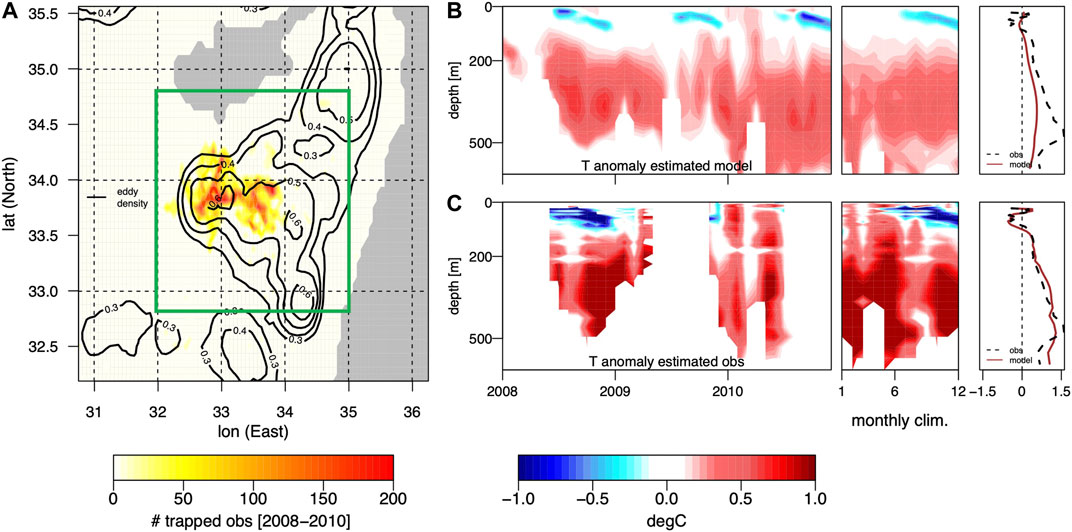
FIGURE 2. (A) Number of “eddy-trapped” observations over the period 2008–2010 considering eddies with lifetime ≥ 2 weeks occurring in the Shikmona gyre area (green frame). Black contours show the eddy probability density from the MED-REA, i.e., the probability to find an eddy in the specific area. (B) Three plots showing respectively: the time-series of eddy temperature anomaly from the MED-REA, its monthly climatology, the overall mean of temperature anomaly profile. (C) same as (B) for Argo profiling floats. In this panel, the average anomaly from observations (black dotted line) is compared with the average anomaly from MED-REA values, extrapolated at the observation positions (red line).

Anticyclonic eddies are typically warm-core at depth, however the sharp warming of sea surface water that occurs in the East-Mediterranean sea changes the picture. Figures 2B,C show the temperature anomaly calculated using the eddy detection system applied to the MED-REA and in-situ ARGO observations, respectively. For each panel, three different temporal averages are displayed: the first panel shows the time-series of monthly anomaly from 2008 to 2011, the second corresponds to the monthly climatology of the anomaly, while the third shows the vertical mean profile of anomaly only in the presence of an eddy. The water trapped by ACE is generally warmer at depth, however starting from August, a dipole-like structure of the anomaly tends to appear both in the MED-REA and in the observations. The water trapped in August is colder at the top and warmer at the bottom. During fall, the cold anomaly tends to drift down reaching about 100 m in winter before disappearing. The same trend can be seen both in the observations and in the re-analysis, but the method tends to underestimate the anomaly in magnitude compared to the observations. Here it is worth keeping in mind that the algorithm evaluates the total anomaly by averaging over the eddy area, while observations are point-wise measurements. Calculating the anomaly using the model temperature at the observation positions, the model-based anomaly profiles closely follow those in the observations, as it can be noticed by comparing black and red lines in Figure 2C. Note that although the EN4 dataset is not directly assimilated, Argo profiles are assimilated during the ocean re-analysis integration.

Such a peculiar structure of the anomaly inside the eddy can be visually inspected in the temperature field of August 2008. Figure 3 shows the zonal sections of the temperature field for the re-analysis and an observation-derived product, called ARMOR3D (Guinehut et al., 2012; Mulet et al., 2012), at the eddy position. ARMOR3D is a statistical three-dimensional reconstruction of several physical variables that employs only observations (T, S, SST) at a resolution of 1/4°. The presence of a cold-core at the top and a warm one at the bottom (300 m) is present in the two datasets. In ARMOR3D the center of the eddy is moved slightly north and is larger compared to the re-analysis, probably due to the dataset’s coarser resolution. The same picture can be seen looking at the vertical temperature profiles from in-situ observations for the same month (Figure 3C). Mauri et al. (2019), analysing the data of two cruises in late 2016 and comparing them with satellite SST data, observe that in August the SST at the core of the eddy is colder than the perimetral water, while at depth the situation reverses. The colder SST signal tends to disappear during fall. The authors suggest that such behavior is probably due to the stiffening of the thermocline in the Eastern Mediterranean Sea in August. The rapid increase of the temperature at the surface leads to an environmental temperature that is, now warmer than the one inside the eddy, where the water parcels tend to be more vertically homogeneous and thermalize slowly. Moreover, despite the anticyclonic behaviour the salinity is higher inside the eddy (Mauri et al., 2019) and reflects its mode-water nature. This is also seen by analyzing the re-analysis with our detection method, as in Figure 8, while the other anticyclones typically show fresher water inside.

FIGURE 3

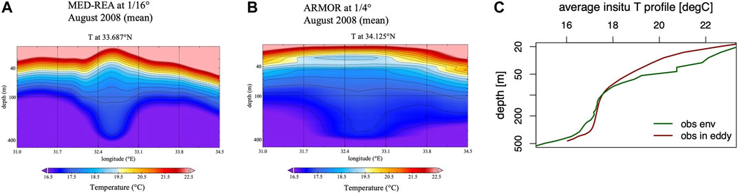
FIGURE 3. Panels (A) and (B) show the monthly zonal sections of temperature in the Shikmona gyre area (green-box in Figure 2) for August 2008 extracted from two products MED-REA and ARMOR3D respectively. (C) Temperature profiles calculated from in-situ observations occurring in the region (Figure 2) during the same month. In-situ profiles are gathered both inside (trapped) and outside the eddy.

3.2 Eddy Population

It is very well-known that the number of detected eddies can largely change according to the technical details of the detection system in use, and it is therefore extremely important to quantify the impact of possible spurious (or missed) eddies detected on the final results. An eddy miss would lead to underestimating the eddy-driven anomaly in the region; in Section 3.1 the vertical temperature anomaly is compared with the one extracted from point-wise Argo observations in the Shikmona area to estimate the accuracy. A second possible misrepresentation comes from the detection of false-positive eddies that could potentially spoil the calculation of the anomaly. To reduce the impact of such events, in addition to the use of stringent conditions on rotation, lifetime, and depth (see Supplementary Appendix SA), the anomaly content is here defined with respect to the eddy surrounding environment (see Section 2.2.1). The stability of the anomaly signal as a function of the lifetime is also presented to support the results. Therefore the exact numbers in the population should not be taken as an absolute reference but rather as a relative one, comparing results for different lifetimes.

Eddy population is defined in terms both of the occurrence and persistence of non-linear structures in the Mediterranean basin. Different lifetimes are shown to stress the contribution of eddies that preserve their properties while spanning over different temporal scales.

During the 24 years analysed, the number of eddies does not seem to show any global statistically-significant trend. Transient eddies/patterns, living a few days only, contribute to the high-frequency variability in the statistics where short-living eddies are included. The population of short-living eddies is probably affected by the strength of transient wind and the variability of mixed-layer-depth. Patterns whose vertical extension is not stably deeper than the mixed layer depth contribute to this day-by-day variability. The impact of the variability generated by short-living eddies is out of the scope of the present study that is, mainly focused on the stable signal generated by eddies rather than their variability. Eddies lasting more than 2 weeks are characterized by an average thickness of ∼400 m and by a radius of 45 km (Figure 4), while anti-cyclonic structures are significantly deeper than cyclonic eddies (Table 1). The average eddy diameter and depth tend to increase with the lifetime, reducing the impact of transient eddies that usually are smaller and shallower. The maximum of deepening occurs in winter when the water is less stratified, while eddies are shallower during summertime, following the variability of the mixed layer depth. Atmospheric forcings can also play a role in the year-by-year variability of long-living eddies as well as sporadic events connected to thermohaline circulation changes (Roether et al., 2014). The conservation of angular momentum is likely to play a role in the opposite seasonality of horizontal and vertical extension: smaller, deeper eddies in winter tend to become larger and shallower in summer.

FIGURE 4

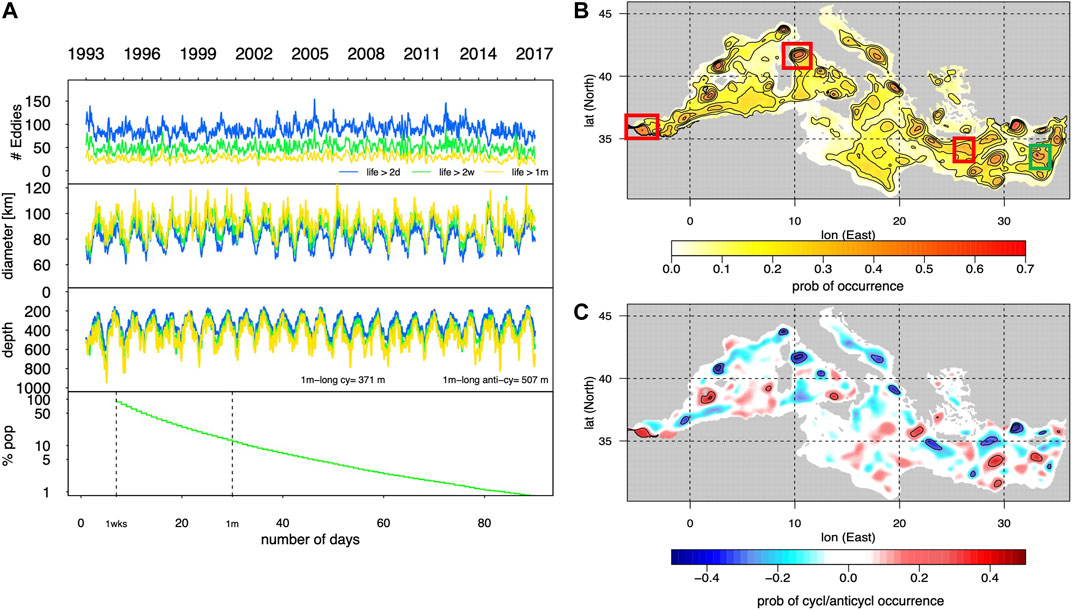
FIGURE 4. Eddy statistics for the Mediterranean Sea: (A) Number of eddies, eddy diameter (km) and eddy depth (m) as a function of lifetime and years. The eddy depth is also given as function of 1 month long lived cyclonic/anticyclonic structures. Eddy decay (% pop.) as a function of lifetime. Probability of eddy occurrence (B) and CE versus ACE (C); frames show the areas of the Alboran, North Tyrrhenian, Ierapetra (red frames), and Shikmona (green frame) gyres.

TABLE 1

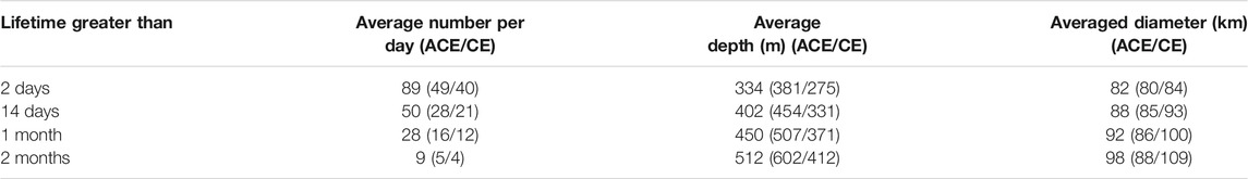
TABLE 1. Average number of eddies persisting per day, their mean depth and mean diameter as function of lifetime and type (ACE/CE).

The bottom panel in Figure 4A shows the percentage of eddy population as a function of their minimum lifetime (in abscissa) starting from eddies living more than 7 days. The population reduces from 50 to 20% down to 2.5% for structures living longer than 2 weeks, 1 month, 2-months, respectively.

The mean spatial distribution of eddies longer than 14 days, is shown in the upper-right panel (Figure 4) as the probability of eddy occurrence (density probability). The areas of the main quasi-stationary eddies are well represented with more than 60–70% probability. The mean spatial distribution of eddy polarity weighted by the eddy density is shown in the lower-left panel (Figure 4). We use eddy density as a weight to remove low-density areas that show strong polarity, but that are not statistically reliable: e.g., eddy polarity tends to zero in low-density areas or areas with high-density but weak polarity.

A strong polarity signal is retained by the well-known quasi-stationary eddies. The overall mesoscale polarity field agrees well with the knowledge of Mediterranean surface/subsurface circulation (e.g., Pinardi et al., 1997) and observations of mesoscale variability (Fusco et al., 2003).

Non-linear features with lifetimes ≥ 2 days were considered as a reference to assess the eddy population as a function of the lifetime. In particular, the ratio between the number of eddies detected at the relevant lifetime and those in the reference provides evidence about the portion of the eddy population that tends to dissipate over different temporal scales. Figure 5 shows the percentage of un-dissipated eddies, obtained considering 3D non-linear features with lifetimes longer than 14 and 28 days, compared to the reference (lifetime ≥ 2 days). In the Figure, a value of 50% means that, for a specific lifetime, the eddy population is half of the total number of eddies with lifetimes ≥ 2 days. It is evident that the eddy population in the Mediterranean Sea is well described by eddies lasting at least 14 days, while long-lived (≥ 28 days) features tend to persist in the eastern part of the basin. Starting from those results, mesoscale structures with lifetimes ≥ 14 days were taken into account to look at the 2D expressions and 3D structure of the eddy population in the Mediterranean Sea.

FIGURE 5

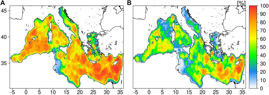
FIGURE 5. The percentage of un-dissipated eddies, considering non-linear structures with lifetimes of at least 14 days (A) and 28 days (B), compared to those with a lifetime of at least 2 days during the 24-year period 1993–2016.

3.3 Dynamic Contributions

In this Section, we investigate the contribution of mesoscale eddies to ocean dynamics by looking at their signature in the SSH variability and EKE. Eddy detection methods rely on the surface expression of mesoscale features. Those can be identified from satellite altimetry maps as elevations (ACE) and depressions (CE) of the sea surface. As such, it is interesting to understand how the SSH variability can be influenced by eddies at temporal and spatial scales which depend on the eddy structures and lifetimes. Figure 6 shows the percentage of the variance of the SSH variability explained by eddies, over the period 1993–2106. The results were obtained by comparing the initial SSH fields with the background (Section 2) and considering eddy lifetimes ≥ 14 and 28 days. The values are expressed as the percentage decrease of the variance in the background with respect to the initial fields. A value of 50% means that the variance of the SSH fields in the background has halved with respect to initial fields. The results clearly show how the signature of mesoscale eddies characterizes the SSH variability. Eddies with a lifetime ≥ 14 days (left panel) explain more than 50% of the variance of the signal both in the western Mediterranean Sea (e.g., Alboran Gyre and the Tyrrhenian Sea) and in the Levantine basin, where the largest values were observed in the occurrence of the Ierapetra, Mersa Matruh and Shikmona gyres. It is interesting to notice that long-lived eddies (≥ 28 days; right panel) show similar values, thus indicating that mesoscale features characterize the SSH variability over temporal scales longer than months.

FIGURE 6

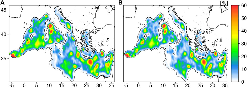
FIGURE 6. The percentage of variance of sea-surface height variance explained by eddies. The panels show the percentage of variance explained by eddies with a lifetime of 14 (A) and 28 days (B), during the 24-year period from 1993 to 2016.

A 3D eddy detection method allows to depict both the horizontal and vertical structure of the mesoscale features and to quantify their contribution to the ocean dynamics, as long as the EKE vanishes in the water column due to dissipation. To assess how the mesoscale variability observed at the ocean surface projects into the 3D ocean circulation, in this Section we look at the EKE driven by the non-linear eddies. Following the approach proposed by Cipollone et al. (2017), who extended the formulation of relative kinetic energy in Chelton et al. (2011b) to take into account 3D structures, we consider the relative EKE (REKE) to represent the fraction of ocean kinetic energy carried by eddies in space and time (see Supplementary Appendix SB for further details). Figure 7 shows the REKE associated with mesoscale eddy lifetime ≥ 14 days, both considering their surface expression (left panel) and 3D structure. At the surface, the REKE was up to the order of ≥ 50% looking at the dominant mesoscale features in the Mediterranean basin. The results in Section 3.2, show average eddy depths of 500 m (Table 1). The latter was used as a reference depth to consider 3D eddy contributions. Looking at vertically integrated REKE values, it is possible to appreciate the differences between the western and eastern parts of the Mediterranean basin. The largest REKE values were observed in the occurrence of the Pelops (ACE), Ierapetra (ACE), Rhodes (CE), Mersa Mathru (ACE), Shikmona gyres (ACE). Those are well-known quasi-stationary mesoscale features in the Levantine Basin (e.g., Pinardi et al., 2005), reaching hundreds of meters into the water column (e.g., Fusco et al., 2003). The absolute EKE values (cm²/s²) driven by eddies occurring in specific areas of the Mediterranean Sea (red and green boxes in Figure 4) are shown in Table 2. In particular, the largest REKE values (30–40%) at depth were observed in the areas of the Ierapetra and Shikmona gyres. This is in line with the typical characteristic of ACEs, associated with pycnocline depressions, which tend to penetrate deeper in the water column compared to CEs (e.g., Rhines, 2001).

FIGURE 7

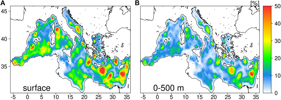
FIGURE 7. REKE at the surface (A) and the 3D structure to 500 m (B) expressed in percentage (%). The panels are obtained over a 24-year period, from 1993 to 2016, for eddies with a lifetime geq 14 days.

TABLE 2

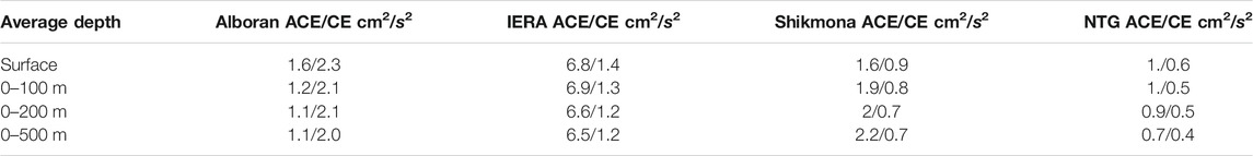
TABLE 2. Absolute value of EKE trapped by the eddies occurring in different regions of the Mediterranean Sea and averaged over different depths. Eddies with lifetime greater than 2 weeks are used.

Eddy Driven 3D Anomalies and Thermodynamic Contributions

ACE and CE are typically associated with warm and cold temperature anomalies (e.g., Dong et al., 2014). Cyclonic eddies induce negative anomalies of temperature and/or positive anomalies of salinity and therefore positive anomalies of density. This is because cyclones tend to uplift the pycnocline. The effect is the opposite for anticyclonic eddies which lower the pycnocline. The maximum of the anomalies is also deeper for anticyclones. The lowered pycnocline in anticyclones will create a maximum of the temperature anomaly below the mean depth of the pycnocline whereas an uplifted pycnocline in cyclones will create a minimum above. This behaviour can be reflected in the mesoscale eddies of the western Mediterranean, for example, in the Alboran and Tyrrhenian Seas, while interesting departures can be observed in the eastern part of the basin.

Panels in Figure 8 show the ACE/CE anomalies for different variables and selected regions: Alboran gyre (ALB), Shikmona area (SHIK), Ierapetra gyre (IERA), and North Tyrrhenian Gyre (NTG), as depicted in Figure 4. For each region, we separate contributions from ACE and CE eddies and calculate the anomaly in T, S, rotational velocity (v_R) and REKE. The monthly time series of the anomaly is then shown from 1993 to 2016 together with the monthly climatology of the anomaly and the mean anomaly profile inside the eddy. While the monthly climatology includes also months without eddies and provides the mean anomaly for each month, the last mean profile shows different information being calculated only in the case the eddy is present. This can be seen as the typical signature of the eddy in the case of its appearance at a specific depth.

FIGURE 8

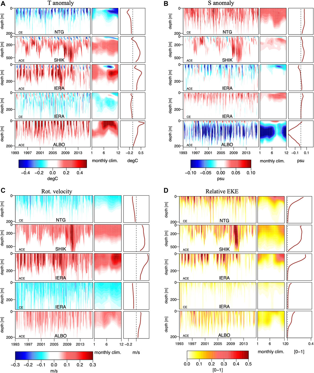
FIGURE 8. Time series of eddy-driven anomalous profile calculated in different regions (North Tyrrhenian Gyre–NTG, Shikmona area–SHIK, Ierapetra region–IERA, and Alboran Gyre–ALBO) for different variables: (A) temperature, (B) salinity, (C) rotational velocity, and (D) REKE. In the IeraPetra region, both ACE and CE contributions are shown. For each time series, the monthly climatology of the anomalous profiles and the mean eddy anomalous profiles are also shown. The latter is not averaged over months without eddies, only trapped waters contribute.

In the western part of the basin, the Alboran gyre, made of at least two semi-permanent structures which tend to be predominant according to the seasons (e.g., Escudier et al., 2016), plays a fundamental role in modulating the entrance of the Atlantic waters into the Mediterranean Sea (Pinardi et al., 2015). Here we focus our attention on the westernmost anticyclonic structure (hereafter referred to as ALBO), which resides in the Alboran Sea irrespective of the season considered (Figure 4). As expected looking at ACEs, the ALBO shows specific properties characterized by warmer (fresher) temperature (salinity) anomalies. Looking at the temporal evolution (1993–2016) of the eddy-driven anomalies (left panels) it is also possible to investigate their contributions over different seasons. In Figure 8, central panels show the eddy-driven anomalies as a climatology. Salinity anomalies in ALBO were negative from December to April, around 0.2 psu. The Alboran Sea is characterized by fresher Atlantic waters at the surface and denser water at the bottom exiting the Mediterranean Sea. Water masses stratification varies seasonally, due to wind-driven circulation and solar radiation, and it is typically higher during summer in the Mediterranean Sea. The water masses trapped in ALBO showed positive salinity anomalies at the surface and negative at depth down to 200 m from May to September.

In the northern Tyrrhenian gyre, a large quasi-stationary CE eddy is almost continuously present. This eddy induces negative anomalies of temperature and positive anomalies of salinity, uplifting the pycnocline and tending to strengthen in late summer/autumn exceeding the −0.5°C value.

The REKE profile is typical of a bowl-shape eddy while tracer anomalies can reach down to ∼150 m that can be interpreted as the eddy “trapping depth,” usually defined as the vertical extent of the trapped fluid inside the eddy (e.g., Chaigneau et al., 2011). No relevant ACE are detected in this region. The peculiar eddy-driven temperature anomaly profile of the Shikmona ACE is already discussed in the dedicated Section and compared with the literature results. This ACE is a mode-water eddy that differs from the standard ACE showing a positive anomaly in salinity, as demonstrated by two recent field campaigns (Mauri et al., 2019). The rotational speed that constrains the water masses trapped by the eddy is about 0.2 m/s in all the seasons, being almost uniform down to 300 m. The REKE profiles show that it contributes to the EKE of the regions with more than 30% down to 300 m. In the exact position of the eddy, the percentage can rise to 60–70% as seen in the map of REKE (Figure 7).

The sector in the Ierapetra region (Figure 4) is characterised by high-mesoscale activity with a strong quasi-stationary ACE, continuously detected in almost all the months. The presence of such ACE has been demonstrated in several oceanographic cruises and analysing satellite altimetry data (Ioannou et al., 2017; Ioannou et al., 2019). It can be inferred that a positive temperature anomaly, higher than 0.5°C, persists in all the seasons at depth. The same mechanism that generates a negative summertime temperature anomaly in the Shikmona ACE, and described in the dedicated Section, seems to be present in this area. In the late summer/autumn season the SST in the Eastern Mediterranean sea is characterized by abrupt heating that stiffens the stratification and leads to an environmental temperature that in a short time becomes higher than water temperature in the ACE. The latter tends to be more uniform acting against the stratification, i.e., the temperature inside ACE is rather homogeneous while the environmental one is strongly stratified and generates the vertical dipole structure in the anomaly content. The standard ACE behavior is recovered in winter and spring. Such dipole is not seen in the salinity, which shows mainly negative and very shallow anomalies compared to the temperature. Looking at the REKE anomaly, it is interesting to notice that the profile differs from the bowl-shape structure typically associated with NTG CE and reaches a trapping depth of 200 m. During 2008 the ACEs were deeper, and also the salinity anomaly at depth tended to change sign. This is in line with the results obtained by Velaoras et al. (2014) who, looking at thermohaline circulation in the Cretan Sea, observed a large outflow of dense waters from the Aegean to the Cretan Sea over the period 2007–2009. The authors argued that this was an Eastern Mediterranean Transient (EMT; Roether et al., 2014; Pinardi et al., 2019) - like event connected to thermohaline circulation changes, instead of being driven by atmospheric forcings or water fluxes. The CE in the same regions shows an opposite behavior of ACE although the anomaly is smaller in magnitude (0.2°C).

Mesoscale eddies can act as gateways for heat absorption and loss in the ocean. It is then interesting to quantify how eddy-driven anomalies affect the ocean heat content (OHC). At a depth range between 0 and 700 m, the OHC in the Mediterranean Sea was in the order of 10⁹ J m⁻² (basin integral over the period 1993–2016; not shown), in agreement with the already existing estimates for the Mediterranean basin (von Schuckmann et al., 2016; Iona et al., 2018). Considering those initial estimates as a reference, Figure 9 shows the OHC anomalies obtained considering long-lived eddies (≥ 4 weeks). In particular, the values are expressed as a percentage (%) of total ocean heat content monthly standard deviation, obtained integrating MED-REA ocean temperature fields over different depth ranges. Considering a depth range between 0 and 100 m, the mesoscale contributions to the OHC in the Mediterranean Sea were in the order of 20%. Positive (negative) contributions reflected the characteristics of ACE (CE) eddies, acting as warm (cold) cores and thus underlying their role in modulating the magnitude OHC in the upper ocean. As already discussed in Section 3.3, a maximum depth of 500 m was selected to look at 3D eddy-driven anomalies. At this depth range, contributions up to 15% were observed in the occurrence of the most prominent mesoscale features.

FIGURE 9

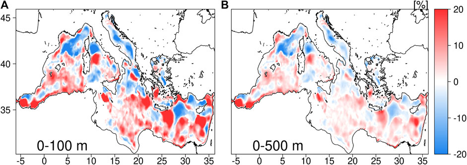
FIGURE 9. Eddy-driven ocean heat content anomalies versus depth derived from MED-REA temperature fields. The panels show the results obtained over a 24-years (1993–2016) period considering eddies with a lifetime of at least 4 weeks. Values are expressed as a percentage (%) of total ocean heat content monthly standard deviation.

FIGURE 10

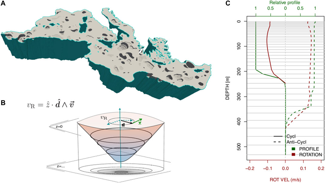
FIGURE 10. (A) Example of one-week-long eddy population detected in 1 day. (B) Schematic illustration of vertical change in orbital velocity. (C) Examples of relative vertical profile (green) generated by the rotational velocity v_R (red color) for cyclonic (solid line) and anti-cyclonic (dashed) eddy at each vertical level. The relative vertical profile shows the vertical inner shape of the eddy defined by its area at each vertical level, normalized by the area at the surface. It is therefore always 1 at the surface and 0 at the bottom; the vertical line going from 1 to 0 corresponds to the eddy shape segmented by the detection system.

4 Concluding Discussion

The eddy population in the Mediterranean Sea was investigated by means of eddy detection and tracking algorithms applied to the 3D dimensional ocean fields from MED-REA over a 24-year period (1993–2016). In particular, we focused on the contributions to ocean dynamics and thermodynamics of eddy-induced anomalies. Mesoscale eddies are non-linear features of the circulation showing properties that may differ from the surrounding waters as a function of their spatial and temporal scales.

To remove any bias arising from the use of a climatological background, in this work eddy-driven anomalies were defined with respect to the non-homogeneous surrounding waters.

The accuracy of the method, to disclose the 3D mesoscale contributions, was assessed against Argo profiling floats trapped by eddies as well as from the observation-based data sets (i.e., ARMOR3D).

The eddy population in the Mediterranean Sea was characterized according to the occurrence and persistence of non-linear structures. Tracking the eddies, the results showed that structures living ≥ 2 weeks are representative of the 3D mesoscale field in the basin, showing a high probability (> 60%) of occurrence in the areas of the main quasi-stationary eddies. The emerging mesoscale polarity (ACEs/CEs) field was in line with previous model and observation-based studies (Pinardi et al., 1997; Fusco et al., 2003; Escudier et al., 2016) with an average thickness of ∼400 m and a radius of 45 km. The results also showed the dependency of eddies size and thickness to polarity and lifetime. ACEs were significantly deeper than CEs and the average eddy diameter and thickness tended to increase in long-lived structures. Eddy thickness shows also seasonal variability: eddies tend to be shallower in stratified waters during summer and deeper during winter. Looking at eddies as a function of their lifetime, the results showed how the eddy population decreases to 20% considering long-lived structures (e.g., ≥ 1 month). The contribution of mesoscale eddies to the ocean dynamics was assessed by investigating their surface expression and 3D structure. At the surface, the signature of mesoscale features explained most of the variance of the SSH field, showing significant contributions at temporal scales longer than 1 month. Mesoscale eddies drive a large portion of the kinetic energy in the Mediterranean Sea, and REKE values were larger than 50–60% both at the surface and at depth (e.g., in the area of Shikmona gyre).

Vertical profiles of velocity and REKE are shown for several areas and the trapping depth is discussed. Looking at the contributions to the ocean thermodynamics, the results exhibit the existence of typical warm (cold) cores associated with ACEs (CEs), with the relevant exception in the area of the Shikmona gyre that shows a structure which is closer to a mode-water ACE eddy with a positive salinity anomaly. This result seems to be confirmed by several oceanographic cruises (Mauri et al., 2019). The vertical temperature anomalies of eastern Mediterranean eddies are affected by a strong summer stratification in the surface water, showing an opposite sign of the anomaly whether looking at surface or at depth. A dedicated comparison against Argo floats in the Shikmona area has been performed to confirm such behavior together with a comparison with observation-only ocean reconstructions. In late 2008, there is a deepening of the Ierapetra gyre that coincides with a well-known large outflow of dense waters from the Aegean sea (EMT-like event, Velaoras et al., 2014).

Mesoscale contributions to ocean thermodynamics were assessed looking at the OHC. The results show that the temperature anomalies of long-lived eddies (≥ 4 weeks) account for up to the 15–25% of the OHC monthly variability in the upper ocean.

During the development of this work, a new high-resolution (1/24°) realization of the MED-REA was achieved, and it is currently distributed through the CMEMS data portal (Escudier et al., 2020). New approaches, based on machine-learning (ML) methods, to detect and reconstruct mesoscale structures from observations (e.g., Moschos et al., 2020) and models (George et al., 2021) were also developed recently. In this sense, the proposed method can represent the foundation for creating training data sets for ML-based and transfer-learning methods (e.g., Kadow et al., 2020) to reconstruct the 3D mesoscale field in the ocean emerging from the synergy between multi-platform observations and multiple eddy-resolving ocean syntheses.

Data Availability Statement

The raw data supporting the conclusion of this article will be made available by the authors on request.

Author Contributions

AB and AC conducted all the analyses and wrote the paper. JJ and JS reviewed the whole manuscript. RR and AA commented on a preliminary draft and contributed to finalizing the manuscript.

Funding

This collaborative study was supported through the Bjerknes Center for Climate Research (BCCR) initiative for strategic projects.

Conflict of Interest

The authors declare that the research was conducted in the absence of any commercial or financial relationships that could be construed as a potential conflict of interest.

The handling editor declared a past co-authorship with several of the authors AB, AC.

Publisher’s Note

All claims expressed in this article are solely those of the authors and do not necessarily represent those of their affiliated organizations, or those of the publisher, the editors and the reviewers. Any product that may be evaluated in this article, or claim that may be made by its manufacturer, is not guaranteed or endorsed by the publisher.

Acknowledgments

We acknowledge the CINECA award under the ISCRA initiative for the availability of high-performance computing resources and support. The analyses were also performed using the highperformance computer at Helmholtz Zentrum Hereon. JS gratefully acknowledges the support by the H2020 Project IMMERSE.

Supplementary Material

The Supplementary Material for this article can be found online at: https://www.frontiersin.org/articles/10.3389/feart.2021.724879/full#supplementary-material

References

Alhammoud, B., Béranger, K., Mortier, L., Crépon, M., and Dekeyser, I. (2005). Surface Circulation of the Levantine Basin: Comparison of Model Results With Observations. Prog. Oceanography 66, 299–320. doi:10.1016/j.pocean.2004.07.015

CrossRef Full Text | Google Scholar

Ashkezari, M. D., Hill, C. N., Follett, C. N., Forget, G., and Follows, M. J. (2016). Oceanic Eddy Detection and Lifetime Forecast Using Machine Learning Methods. Geophys. Res. Lett. 43, 234–312. doi:10.1002/2016GL071269

CrossRef Full Text | Google Scholar

Ayoub, N., Le Traon, P.-Y., and De Mey, P. (1998). A Description of the Mediterranean Surface Variable Circulation From Combined Ers-1 and Topex/poseidon Altimetric Data. J. Mar. Syst. 18, 3–40. doi:10.1016/s0924-7963(98)80004-3

CrossRef Full Text | Google Scholar

Balmaseda, M. A., Hernandez, F., Storto, A., Palmer, M. D., Alves, O., Shi, L., et al. (2015). The Ocean Reanalyses Intercomparison Project (ORA-IP). J. Oper. Oceanography 8, s80–s97. doi:10.1080/1755876X.2015.1022329

CrossRef Full Text | Google Scholar

Barceló-Llull, B., Sangrà, P., Pallàs-Sanz, E., Barton, E. D., Estrada-Allis, S. N., Martínez-Marrero, A., et al. (2017). Anatomy of a Subtropical Intrathermocline Eddy. Deep Sea Res. Oceanographic Res. Pap. 124, 126–139. doi:10.1016/j.dsr.2017.03.012

CrossRef Full Text | Google Scholar

Bonaduce, A., Benkiran, M., Remy, E., Le Traon, P. Y., and Garric, G. (2018). Contribution of Future Wide-Swath Altimetry Missions to Ocean Analysis and Forecasting. Ocean Sci. 14, 1405–1421. doi:10.5194/os-14-1405-2018

CrossRef Full Text | Google Scholar

Chaigneau, A., Le Texier, M., Eldin, G., Grados, C., and Pizarro, O. (2011). Vertical Structure of Mesoscale Eddies in the Eastern South Pacific Ocean: A Composite Analysis from Altimetry and Argo Profiling Floats. J. Geophys. Res. 116. doi:10.1029/2011JC007134

CrossRef Full Text | Google Scholar

Chelton, D. B., Gaube, P., Schlax, M. G., Early, J. J., and Samelson, R. M. (2011a). The Influence of Nonlinear Mesoscale Eddies on Near-Surface Oceanic Chlorophyll. Science 334, 328–332. doi:10.1126/science.1208897

PubMed Abstract | CrossRef Full Text | Google Scholar

Chelton, D. B., Schlax, M. G., and Samelson, R. M. (2011b). Global Observations of Nonlinear Mesoscale Eddies. Prog. Oceanography 91, 167–216. doi:10.1016/j.pocean.2011.01.002

CrossRef Full Text | Google Scholar

Chelton, D. B., Schlax, M. G., Samelson, R. M., and de Szoeke, R. A. (2007). Global Observations of Large Oceanic Eddies. Geophys. Res. Lett. 34, L15606. doi:10.1029/2007GL030812

CrossRef Full Text | Google Scholar

Chen, G., Chen, X., and Huang, B. (2021). Independent Eddy Identification With Profiling Argo as Calibrated by Altimetry. J. Geophys. Res. Oceans. 126, e2020JC016729. doi:10.1029/2020JC016729

CrossRef Full Text | Google Scholar

Cipollone, A., Masina, S., Storto, A., and Iovino, D. (2017). Benchmarking the Mesoscale Variability in Global Ocean Eddy-Permitting Numerical Systems. Ocean Dyn. 67, 1313–1333. doi:10.1007/s10236-017-1089-5

CrossRef Full Text | Google Scholar

Dee, D. P., Uppala, S. M., Simmons, A. J., Berrisford, P., Poli, P., Kobayashi, S., et al. (2011). The ERA-Interim Reanalysis: Configuration and Performance of the Data Assimilation System. Q.J.R. Meteorol. Soc. 137, 553–597. doi:10.1002/qj.828

CrossRef Full Text | Google Scholar

Dobricic, S., and Pinardi, N. (2008). An Oceanographic Three-Dimensional Variational Data Assimilation Scheme. Ocean Model. 22, 89–105. doi:10.1016/j.ocemod.2008.01.004

CrossRef Full Text | Google Scholar

Doglioli, A. M., Blanke, B., Speich, S., and Lapeyre, G. (2007). Tracking Coherent Structures in a Regional Ocean Model With Wavelet Analysis: Application to Cape basin Eddies. J. Geophys. Res. 112. doi:10.1029/2006JC003952

CrossRef Full Text | Google Scholar

Dong, C., Lin, X., Liu, Y., Nencioli, F., Chao, Y., Guan, Y., et al. (2012). Three-dimensional Oceanic Eddy Analysis in the Southern california Bight from a Numerical Product. J. Geophys. Res. 117, a–n. doi:10.1029/2011JC007354

CrossRef Full Text | Google Scholar

Dong, C., McWilliams, J. C., Liu, Y., and Chen, D. (2014). Global Heat and Salt Transports by Eddy Movement. Nat. Commun. 5, 3294. doi:10.1038/ncomms4294

PubMed Abstract | CrossRef Full Text | Google Scholar

Drévillon, M., Bourdallé-Badie, R., Derval, C., Lellouche, J. M., Rémy, E., Tranchant, B., et al. (2008). The GODAE/Mercator-Ocean Global Ocean Forecasting System: Results, Applications and Prospects. J. Oper. Oceanography 1, 51–57. doi:10.1080/1755876X.2008.11020095

CrossRef Full Text | Google Scholar

Duo, Z., Wang, W., and Wang, H. (2019). Oceanic Mesoscale Eddy Detection Method Based on Deep Learning. Remote Sensing 11, 1921. doi:10.3390/rs11161921

CrossRef Full Text | Google Scholar

Escudier, R., Clementi, E., Omar, M., Cipollone, A., Pistoia, J., Aydogdu, A., et al. (2020). Mediterranean Sea Physical Reanalysis (Version 1) [Data Set]. Copernicus Monit. Environ. Mar. Serv. (Cmems). doi:10.25423/CMCC/MEDSEA_MULTIYEAR_PHY_006_004_E3R1

CrossRef Full Text | Google Scholar

Escudier, R., Renault, L., Pascual, A., Brasseur, P., Chelton, D., and Beuvier, J. (2016). Eddy Properties in the Western Mediterranean Sea From Satellite Altimetry and a Numerical Simulation. J. Geophys. Res. Oceans 121, 3990–4006. doi:10.1002/2015JC011371

CrossRef Full Text | Google Scholar

Faghmous, J. H., Frenger, I., Yao, Y., Warmka, R., Lindell, A., and Kumar, V. (2015). A Daily Global Mesoscale Ocean Eddy Dataset from Satellite Altimetry. Sci. Data. 2, 150028. doi:10.1038/sdata.2015.28

PubMed Abstract | CrossRef Full Text | Google Scholar

Fernández, V., Dietrich, D. E., Haney, R. L., and Tintoré, J. (2005). Mesoscale, Seasonal and Interannual Variability in the Mediterranean Sea Using a Numerical Ocean Model. Prog. Oceanography 66, 321–340. doi:10.1016/j.pocean.2004.07.010

CrossRef Full Text | Google Scholar

Frenger, I., Münnich, M., Gruber, N., and Knutti, R. (2015). Southern OCean Eddy Phenomenology. J. Geophys. Res. Oceans 120, 7413–7449. doi:10.1002/2015JC011047

CrossRef Full Text | Google Scholar

Fusco, G., Manzella, G. M. R., Cruzado, A., Gačić, M., Gasparini, G. P., Kovačević, V., et al. (2003). Variability of Mesoscale Features in the Mediterranean Sea from Xbt Data Analysis. Ann. Geophys. 21, 21–32. doi:10.5194/angeo-21-21-2003

CrossRef Full Text | Google Scholar

Gaube, P., Chelton, D. B., Strutton, P. G., and Behrenfeld, M. J. (2013). Satellite Observations of Chlorophyll, Phytoplankton Biomass, and Ekman Pumping in Nonlinear Mesoscale Eddies. J. Geophys. Res. Oceans 118, 6349–6370. doi:10.1002/2013jc009027

CrossRef Full Text | Google Scholar

Gaube, P., McGillicuddy, D. J., Chelton, D. B., Behrenfeld, M. J., and Strutton, P. G. (2014). Regional Variations in the Influence of Mesoscale Eddies on Near-Surface Chlorophyll. J. Geophys. Res. Oceans 119, 8195–8220. doi:10.1002/2014jc010111

CrossRef Full Text | Google Scholar

George, T. M., Manucharyan, G. E., and Thompson, A. F. (2021). Deep Learning to Infer Eddy Heat Fluxes From Sea Surface Height Patterns of Mesoscale Turbulence. Nat. Commun. 12, 1–11. doi:10.1038/s41467-020-20779-9

PubMed Abstract | CrossRef Full Text | Google Scholar

Good, S. A., Martin, M. J., and Rayner, N. A. (2013). EN4: Quality Controlled Ocean Temperature and Salinity Profiles and Monthly Objective Analyses With Uncertainty Estimates. J. Geophys. Res. Oceans 118, 6704–6716. doi:10.1002/2013JC009067

CrossRef Full Text | Google Scholar

Guinehut, S., Dhomps, A.-L., Larnicol, G., and Le Traon, P.-Y. (2012). High Resolution 3-D Temperature and Salinity fields Derived from In Situ and Satellite Observations. Ocean Sci. 8, 845–857. doi:10.5194/os-8-845-2012

CrossRef Full Text | Google Scholar

Hallberg, R. (2013). Using a Resolution Function to Regulate Parameterizations of Oceanic Mesoscale Eddy Effects. Ocean Model. 72, 92–103. doi:10.1016/j.ocemod.2013.08.007

CrossRef Full Text | Google Scholar

Haza, A. C., Özgökmen, T. M., Griffa, A., Garraffo, Z. D., and Piterbarg, L. (2012). Parameterization of Particle Transport at Submesoscales in the Gulf Stream Region Using Lagrangian Subgridscale Models. Ocean Model. 42, 31–49. doi:10.1016/j.ocemod.2011.11.005

CrossRef Full Text | Google Scholar

Heimbach, P., Fukumori, I., Hill, C. N., Ponte, R. M., Stammer, D., Wunsch, C., et al. (2019). Putting it All Together: Adding Value to the Global Ocean and Climate Observing Systems With Complete Self-Consistent Ocean State and Parameter Estimates. Front. Mar. Sci. 6, 55. doi:10.3389/fmars.2019.00055

CrossRef Full Text | Google Scholar

Ioannou, A., Stegner, A., Le Vu, B., Taupier-Letage, I., and Speich, S. (2017). Dynamical Evolution of Intense Ierapetra Eddies on a 22 Year Long Period. J. Geophys. Res. Oceans. 122, 9276–9298. doi:10.1002/2017jc013158

CrossRef Full Text | Google Scholar

Ioannou, A., Stegner, A., Tuel, A., LeVu, B., Dumas, F., and Speich, S. (2019). Cyclostrophic Corrections of Aviso/Duacs Surface Velocities and its Application to Mesoscale Eddies in the Mediterranean Sea. J. Geophys. Res. Oceans. 124, 8913–8932. doi:10.1029/2019JC015031

CrossRef Full Text | Google Scholar

Iona, A., Theodorou, A., Sofianos, S., Watelet, S., Troupin, C., and Beckers, J.-M. (2018). Mediterranean Sea Climatic Indices: Monitoring Long-Term Variability and Climate Changes. Earth Syst. Sci. Data. 10, 1829–1842. doi:10.5194/essd-10-1829-2018

CrossRef Full Text | Google Scholar

Kadow, C., Hall, D. M., and Ulbrich, U. (2020). Artificial Intelligence Reconstructs Missing Climate Information. Nat. Geosci. 13, 408–413. doi:10.1038/s41561-020-0582-5

CrossRef Full Text | Google Scholar

Lin, X., Dong, C., Chen, D., Liu, Y., Yang, J., Zou, B., et al. (2015). Three-Dimensional Properties of Mesoscale Eddies in the South china Sea Based on Eddy-Resolving Model Output. Deep Sea Res. Part Oceanographic Res. Pap. 99, 46–64. doi:10.1016/j.dsr.2015.01.007

CrossRef Full Text | Google Scholar

Liu, Z., Liao, G., Hu, X., and Zhou, B. (2020). Aspect Ratio of Eddies Inferred From Argo Floats and Satellite Altimeter Data in the Ocean. J. Geophys. Res. Oceans. 125, e2019JC015555. doi:10.1029/2019JC015555

CrossRef Full Text | Google Scholar

Madec, G. (2016). NEMO Ocean Engine Publisher. Institut Pierre-Simon Laplace (IPSL).

Marullo, S., Napolitano, E., Santoleri, R., Manca, B., and Evans, R. (2003). Variability of Rhodes and Ierapetra Gyres During Levantine Intermediate Water Experiment: Observations and Model Results. J. Geophys. Res. 108. doi:10.1029/2002JC001393

CrossRef Full Text | Google Scholar

Mason, E., Ruiz, S., Bourdalle-Badie, R., Reffray, G., García-Sotillo, M., and Pascual, A. (2019). New Insight into 3-d Mesoscale Eddy Properties From Cmems Operational Models in the Western Mediterranean. Ocean Sci. 15, 1111–1131. doi:10.5194/os-15-1111-2019

CrossRef Full Text | Google Scholar

Mauri, E., Sitz, L., Gerin, R., Poulain, P.-M., Hayes, D., and Gildor, H. (2019). On the Variability of the Circulation and Water Mass Properties in the Eastern Levantine Sea Between September 2016-August 2017. Water. 11, 1741. doi:10.3390/w11091741

CrossRef Full Text | Google Scholar

Mkhinini, N., Coimbra, A. L. S., Stegner, A., Arsouze, T., Taupier-Letage, I., and Béranger, K. (2014). Long-Lived Mesoscale Eddies in the Eastern Mediterranean Sea: Analysis of 20 Years of AVISO Geostrophic Velocities. J. Geophys. Res. Oceans. 119, 8603–8626. doi:10.1002/2014JC010176

CrossRef Full Text | Google Scholar

Moschos, E., Schwander, O., Stegner, A., and Gallinari, P. (2020). Deep-SST-Eddies: A Deep Learning Framework to Detect Oceanic Eddies in Sea Surface Temperature Images. In ICASSP 2020 - 2020 IEEE International Conference on Acoustics, Speech and Signal Processing. (ICASSP), 4307–4311. doi:10.1109/icassp40776.2020.9053909

CrossRef Full Text | Google Scholar

Mulet, S., Rio, M.-H., Mignot, A., Guinehut, S., and Morrow, R. (2012). A New Estimate of the Global 3D Geostrophic Ocean Circulation Based on Satellite Data and In-Situ Measurements. Deep Sea Res. Part Topical Stud. Oceanography 77-80, 70–81. doi:10.1016/j.dsr2.2012.04.012

CrossRef Full Text | Google Scholar

Oddo, P., Adani, M., Pinardi, N., Fratianni, C., Tonani, M., and Pettenuzzo, D. (2009). A Nested Atlantic-Mediterranean Sea General Circulation Model for Operational Forecasting. Ocean Sci. 5, 461–473. doi:10.5194/os-5-461-2009

CrossRef Full Text | Google Scholar

Oddo, P., Bonaduce, A., Pinardi, N., and Guarnieri, A. (2014). Sensitivity of the Mediterranean Sea Level to Atmospheric Pressure and Free Surface Elevation Numerical Formulation in NEMO. Geoscientific Model. Development under Rev. doi:10.5194/gmd-7-3001-2014

CrossRef Full Text | Google Scholar

Pegliasco, C., Chaigneau, A., and Morrow, R. (2015). Main Eddy Vertical Structures Observed in the Four Major Eastern Boundary Upwelling Systems. J. Geophys. Res. Oceans. 120, 6008–6033. doi:10.1002/2015jc010950

CrossRef Full Text | Google Scholar

Petersen, M. R., Williams, S. J., Maltrud, M. E., Hecht, M. W., and Hamann, B. (2013). A Three-Dimensional Eddy Census of a High-Resolution Global Ocean Simulation. J. Geophys. Res. Oceans. 118, 1759–1774. doi:10.1002/jgrc.20155

CrossRef Full Text | Google Scholar

Pinardi, N., Cessi, P., Borile, F., and Wolfe, C. L. P. (2019). The Mediterranean Sea Overturning Circulation. J. Phys. Oceanography 49, 1699–1721. doi:10.1175/jpo-d-18-0254.1

CrossRef Full Text | Google Scholar

Pinardi, N., Korres, G., Lascaratos, A., Roussenov, V., and Stanev, E. (1997). Numerical Simulation of the Interannual Variability of the Mediterranean Sea Upper Ocean Circulation. Geophys. Res. Lett. 24, 425–428. doi:10.1029/96gl03952

CrossRef Full Text | Google Scholar

Pinardi, N., and Masetti, E. (2000). Variability of the Large Scale General Circulation of the Mediterranean Sea From Observations and Modelling: a Review. Palaeogeogr. Palaeoclimatol. Palaeoecol. 158, 153–173. doi:10.1016/s0031-0182(00)00048-1

CrossRef Full Text | Google Scholar

Pinardi, N., Zavatarelli, M., Adani, M., Coppini, G., Fratianni, C., Oddo, P., et al. (2015). Mediterranean Sea Large-Scale Low-Frequency Ocean Variability and Water Mass Formation Rates From 1987 to 2007: A Retrospective Analysis. Prog. Oceanography 132, 318–332. doi:10.1016/j.pocean.2013.11.003

CrossRef Full Text | Google Scholar

Pinardi, N., Zavatarelli, M., Crise, A., and Ravioli, M. (2005). “The Physical, Sedimentary and Ecological Structure and Variability of Shelf Areas in the Mediterranean Sea,”. The Sea. Editors A. R. Robinson, and K. H. Brink, Vol. 14.

Google Scholar

Raj, R. P., Johannessen, J. A., Eldevik, T., Nilsen, J. E. Ø., and Halo, I. (2016). Quantifying Mesoscale Eddies in the Lofoten basin. J. Geophys. Res. Oceans. 121, 4503–4521. doi:10.1002/2016JC011637

CrossRef Full Text | Google Scholar

Raj, R. P., Halo, I., Chatterjee, S., Belonenko, T., Bakhoday‐Paskyabi, M., Bashmachnikov, I., et al. (2020). Interaction Between Mesoscale Eddies and the Gyre Circulation in the Lofoten basin. J. Geophys. Res. Oceans. 125, e2020JC016102. doi:10.1029/2020JC016102

CrossRef Full Text | Google Scholar

Rhines, P. B. (2001). “Mesoscale Eddies,” in Encyclopedia of Ocean Sciences. Editor J. H. Steele (Oxford: Academic Press), 1717–1730. doi:10.1006/rwos.2001.0143

CrossRef Full Text | Google Scholar

Robinson, A. R., and Golnaraghi, M. (1993). Circulation and Dynamics of the Eastern Mediterranean Sea; Quasi-Synoptic Data-Driven Simulations. Deep Sea Res. Part Topical Stud. Oceanography. 40, 1207–1246. doi:10.1016/0967-0645(93)90068-x

CrossRef Full Text | Google Scholar

Robinson, A. R., Leslie, W. G., Theocharis, A., and Lascaratos, A. (2001). Mediterranean Sea Circulation. Encyclopedia ocean Sci. 3, 1689–1705. doi:10.1006/rwos.2001.0376

CrossRef Full Text | Google Scholar

Robinson, A. R., Malanotte-Rizzoli, P., Hecht, A., Michelato, A., Roether, W., Theocharis, A., et al. (1992). General Circulation of the Eastern Mediterranean. Earth-Science Rev. 32, 285–309. doi:10.1016/0012-8252(92)90002-b

CrossRef Full Text | Google Scholar

Roether, W., Klein, B., and Hainbucher, D. (2014). The Eastern Mediterranean Transient. Geophys. Monogr. 202, 75–83. doi:10.1002/9781118847572.ch6

CrossRef Full Text | Google Scholar

Rubio, A., Barnier, B., Jord, G., Espino, M., and Marsaleix, P. (2009). Origin and Dynamics of Mesoscale Eddies in the Catalan Sea (Nw Mediterranean): Insight from a Numerical Model Study. J. Geophys. Res. Oceans. 114, C06009. doi:10.1029/2007jc004245

CrossRef Full Text | Google Scholar

Sasaki, H., Klein, P., Qiu, B., and Sasai, Y. (2014). Impact of Oceanic-Scale Interactions on the Seasonal Modulation of Ocean Dynamics by the Atmosphere. Nat. Commun. 5, 5636. doi:10.1038/ncomms6636

PubMed Abstract | CrossRef Full Text | Google Scholar

Schütte, F., Brandt, P., and Karstensen, J. (2016). Occurrence and Characteristics of Mesoscale Eddies in the Tropical Northeastern Atlantic Ocean. Ocean Sci. 12, 663–685. doi:10.5194/os-12-663-2016

CrossRef Full Text | Google Scholar

Shi, F., Luo, Y., and Xu, L. (2018). Volume and Transport of Eddy‐Trapped Mode Water South of the Kuroshio Extension. J. Geophys. Res. Oceans. 123, 8749–8761. doi:10.1029/2018JC014176

CrossRef Full Text | Google Scholar

Simoncelli, S., Fratianni, C., Pinardi, N., Grandi, A., Drudi, M., Oddo, P., et al. (2019). Mediterranean Sea Physical Reanalysis (CMEMS MED-Physics) [Data Set]. Copernicus: Monitoring Environment Marine Service (CMEMS). doi:10.25423/MEDSEA_REANALYSIS_PHYS_006_004

CrossRef Full Text

Storto, A., Alvera-Azcárate, A., Balmaseda, M. A., Barth, A., Chevallier, M., Counillon, F., et al. (2019). Ocean Reanalyses: Recent Advances and Unsolved Challenges. Front. Mar. Sci. 6, 418. doi:10.3389/fmars.2019.00418

CrossRef Full Text | Google Scholar

Tonani, M., Balmaseda, M., Bertino, L., Blockley, E., Brassington, G., Davidson, F., et al. (2015). Status and Future of Global and Regional Ocean Prediction Systems. J. Oper. Oceanography 8, s201–s220. doi:10.1080/1755876x.2015.1049892

CrossRef Full Text | Google Scholar

Velaoras, D., Krokos, G., Nittis, K., and Theocharis, A. (2014). Dense Intermediate Water Outflow From the Cretan Sea: A Salinity Driven, Recurrent Phenomenon, Connected to Thermohaline Circulation Changes. J. Geophys. Res. Oceans. 119, 4797–4820. doi:10.1002/2014JC009937

CrossRef Full Text | Google Scholar

Velaoras, D., Papadopoulos, V. P., Kontoyiannis, H., Cardin, V., and Civitarese, G. (2019). Water Masses and Hydrography During April and June 2016 in the Cretan Sea and Cretan Passage (Eastern Mediterranean Sea). Deep Sea Res. Part Topical Stud. Oceanography 164, 25–40. doi:10.1016/j.dsr2.2018.09.005

CrossRef Full Text | Google Scholar

von Schuckmann, K., Le Traon, P.-Y., Alvarez-Fanjul, E., Axell, L., Balmaseda, M., Breivik, L.-A., et al. (2016). The Copernicus Marine Environment Monitoring Service Ocean State Report. J. Oper. Oceanography 9, s235–s320. doi:10.1080/1755876X.2016.1273446

CrossRef Full Text | Google Scholar

Wilks, D. S. (2011). “Empirical Distributions and Exploratory Data Analysis,” in Statistical Methods in the Atmospheric Sciences of International Geophysics. Editor D. S. Wilks (Academic Press), Vol. 100, 23–70. doi:10.1016/B978-0-12-385022-5.00003-8

CrossRef Full Text | Google Scholar

Wunsch, C., and Heimbach, P. (2014). Bidecadal Thermal Changes in the Abyssal Ocean. J. Phys. Oceanography 44, 2013–2030. doi:10.1175/jpo-d-13-096.1

CrossRef Full Text | Google Scholar

Xu, C., Shang, X.-D., and Huang, R. X. (2011). Estimate of Eddy Energy Generation/Dissipation Rate in the World Ocean From Altimetry Data. Ocean Dyn. 61, 525–541. doi:10.1007/s10236-011-0377-8

CrossRef Full Text | Google Scholar

Xu, C., Shang, X.-D., and Huang, R. X. (2014). Horizontal Eddy Energy Flux in the World Oceans Diagnosed From Altimetry Data. Sci. Rep. 4, 5316. doi:10.1038/srep05316

PubMed Abstract | CrossRef Full Text | Google Scholar

Zhang, Z., Tian, J., Qiu, B., Zhao, W., Chang, P., Wu, D., et al. (2016). Observed 3D Structure, Generation, and Dissipation of Oceanic Mesoscale Eddies in the South China Sea. Sci. Rep. 6, 24349. doi:10.1038/srep24349

PubMed Abstract | CrossRef Full Text | Google Scholar

Zhang, Z., Zhang, Y., and Wang, W. (2017). Three-Compartment Structure of Subsurface-Intensified Mesoscale Eddies in the Ocean. J. Geophys. Res. Oceans. 122, 1653–1664. doi:10.1002/2016JC012376

CrossRef Full Text | Google Scholar

Zhao, J., Bower, A., Yang, J., Lin, X., and Penny Holliday, N. (2018). Meridional Heat Transport Variability Induced by Mesoscale Processes in the Subpolar North Atlantic. Nat. Commun. 9, 1124. doi:10.1038/s41467-018-03134-x

PubMed Abstract | CrossRef Full Text | Google Scholar