
95% of researchers rate our articles as excellent or good
Learn more about the work of our research integrity team to safeguard the quality of each article we publish.
Find out more
ORIGINAL RESEARCH article
Front. Earth Sci. , 27 August 2021
Sec. Solid Earth Geophysics
Volume 9 - 2021 | https://doi.org/10.3389/feart.2021.717696
This article is part of the Research Topic The Earthquake Cycle: What Do We Know? View all 8 articles
 Keisuke Ariyoshi1*
 Toshinori Kimura1
 Yasumasa Miyazawa1
 Sergey Varlamov1
 Takeshi Iinuma1
 Akira Nagano1
 Joan Gomberg2,3
 Eiichiro Araki1
 Toru Miyama1Kentaro Sueki1Shuichiro Yada1
 Takane Hori1
 Narumi Takahashi4Shuichi Kodaira1
In our recent study, we detected the pore pressure change due to the slow slip event (SSE) in March 2020 at the two borehole stations (C0002 and C0010), where the other borehole (C0006) close to the Nankai Trough seems not because of instrumental drift for the reference pressure on the seafloor to remove non-crustal deformation such as tidal and oceanic fluctuations. To overcome this problem, we use the seafloor pressure gauges of cabled network Dense Oceanfloor Network System for Earthquakes and Tsunamis (DONET) stations nearby boreholes instead of the reference by introducing time lag between them. We confirm that the time lag is explained from superposition of theoretical tide modes. By applying this method to the pore pressure during the SSE, we find pore pressure change at C0006 about 0.6 hPa. We also investigate the impact of seafloor pressure due to ocean fluctuation on the basis of ocean modeling, which suggests that the decrease of effective normal stress from the onset to the termination of the SSE is explained by Kuroshio meander and may promote updip slip migration, and that the increase of effective normal stress for the short-term ocean fluctuation may terminate the SSE as observed in the Hikurangi subduction zone.
Inland dense networks of seismic and geodetic observations have revealed that slow earthquakes occur on the subduction plate boundaries in the shallower and deeper extensions of megathrust earthquake source regions worldwide (e.g., Schwartz and Rokosky, 2007; Obara and Kato, 2016). It is well known that slow earthquakes have longer duration times than regular earthquakes with the same moment release, and are classified into several types according to spatiotemporal scale (Ide et al., 2007). For instance, low-frequency tremor (LFT) and very low-frequency earthquake (VLFE) are detectable from seismometers because of their dominant frequencies of several hertz (Obara, 2002) and 10–100 s period (Ito et al., 2007), respectively. On the other hand, slow slip events (SSE) are thought to release aseismic slip for days to years (e.g., Ide et al., 2007), which would be detected from geodetic observations.
Dense observation networks have revealed the relations between SSE, VLFE and LFT activity. Some of SSE accompany VLFE and LFT as “episodic tremor and slip” (ETS) (Dragert et al., 2001; Obara and Kato, 2016), where SSE fault zones overlap the source regions of VLFE and LFT.
For the shallower source region, slow earthquakes are close to the trench (Figure 1). Recently, seismic observations on the seafloor such as at the DONET (Dense Oceanfloor Network system for Earthquakes and Tsunamis) (e.g., Kaneda et al., 2015; Kawaguchi et al., 2015) and S-net (Seafloor observation network for earthquakes and tsunamis along the Japan Trench) (Aoi et al., 2020) networks have been useful to monitor slow earthquakes in the shallower extension of subduction zones: e.g., LFT (Annoura et al., 2017; Tanaka et al., 2019) and VLFE (Nakano et al., 2018; Nishikawa et al., 2019). Even for the shallower extension far away from the inland observations, VLFEs are still detectable solely from inland observation networks (Takemura et al., 2019) because of their larger magnitudes than LFTs (e.g., Ide et al., 2007). On the other hand, SSEs are not detectable because they lack seismic signals and static crustal deformation decays with distance as r−3, making their signals too small at inland GNSS networks far away from the trench.
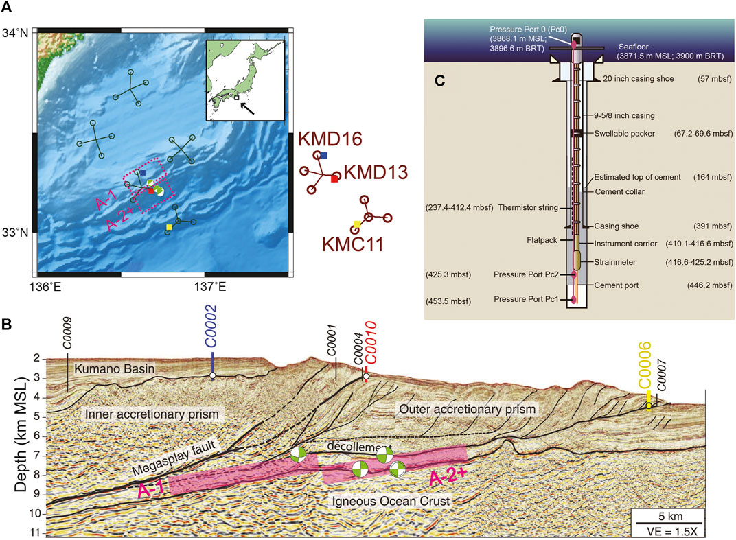
FIGURE 1. (A) Map of the fault model (A-1, A-2+) of the SSE and sVLFE in March 2020 from previous results (Ariyoshi et al., 2021). Squares represent borehole stations. Labeled names (D-16, D-13, and C-11) are the nearby DONET stations for C0002 (blue), C0010 (red), and C0006 (yellow), respectively. Focal mechanism is obtained from Ariyoshi et al. (2021). (B) Seismic section showing the location of the boreholes C0002 (937–980 mbsf), C0010 (610 mbsf), and C0006 (453.5 mbsf), where mbsf = meter below seafloor; VE = vertical exaggeration. The average source location errors of sVLFEs are 5 and 2 km for horizontal and vertical component, respectively (Nakano et al., 2018). Spatial resolution of focal depth and fixed dip angle for the SSE is 1 km and 6°, respectively (Ariyoshi et al., 2021). The focal depths of the fault models A-1 and A-2+ are assumed to be consistent with VLFE because it is practically difficult to determine the focal depth precisely from only the two volumetric strain data at boreholes (C0002 and C0010) by using the simplified green's function. (C) Borehole completion diagram at C0006. The solid magenta ellipses indicate the pressure gauges, where the top one (Pc0) is a hydrostatic reference pressure sensor used to remove oceanographic signals, BRT = below rotary table, and MSL = mean sea level. Figures (B,C) are modified after Figure 1 of Araki et al. (2017) and Figure 2 of Kinoshita et al. (2018), respectively.
Recently, the borehole observatories at C0002, C0010, and C0006 (Figure 1) were successfully connected to DONET (e.g., Araki et al., 2017; Kinoshita et al., 2018). From March 2018, we can monitor crustal deformation at three boreholes along the Nankai Trough in real time. It has been well known that the pore pressure monitoring in boreholes is a useful tool to detect the crustal deformation driven by SSEs (Araki et al., 2017), where the inland observation networks and GNSS-A would not detect it because the fault slip is too small, estimated to be a few centimeters (Ariyoshi et al., 2021).
Figure 2A shows the time series of pore pressure change at boreholes C0002, C0010, and C0006, shown in Figure 1, before and after the SSE in March 2020 (between the black dotted lines). In Figure 2A, the pore pressure change at C0002 is clearly seen as a ramp function. Noting that this characteristic is similar to that observed in the previous SSE in 2015 (Araki et al., 2017), we identified it as an SSE promptly after the occurrence of VLFEs. However, it took several months to estimate the fault model of the SSE (Ariyoshi et al., 2021).
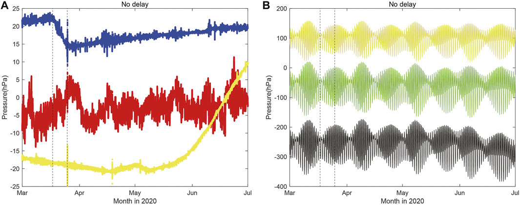
FIGURE 2. Time history of the pore pressure (compression: positive) (A) at the deepest sensors (Pc1) of each borehole observatory (C0002 blue; C0010 red; C0006 yellow), (B) raw data of Pc1 (yellow), Pc0 (black) at C0006 and KMC11 (green). The oceanic signals are canceled out by the reference hydraulic pressure gauge on the seafloor without time delay according to Eq. 1. The vertical lines represent the onset/termination time of the SSE. Offset value for each station is arbitrary and adjusted to see easily.
This difficulty of deriving a fault model is due to the following circumstances. To avoid false recognition, an SSE is identified when significant signals appear at a minimum of two stations. For the SSE shown in Figure 2, we could not find significant signal at C0010 and C0006 due to low ratio of signal to noise in each. To overcome the difficulty, we extract the pore pressure change at C0010 due to crustal deformation by applying t-test between previous record without SSE and volumetric strain change driven by the SSE fault model (Ariyoshi et al., 2021).
Since SSE and VLFE activity is expected to become shorter recurrence interval (Matsuzawa et al., 2010) with greater moment release (Ariyoshi et al., 2014), it would be better to detect SSEs before the occurrence of VLFE toward early warning of megathrust earthquakes and tsunamis. From the analysis of previous SSEs observed from pore pressure in boreholes (Nakano et al., 2018; Ariyoshi et al., 2021), shallow VLFEs (sVLFEs) occur when the SSE migrates upward and its slip reaches the sVLFE source regions, and not so when the SSE region remains in the deeper part. However, we do not know possible factors of promoting slip migration upward. Since slow earthquake including SSE is thought to have stress drop much smaller than regular earthquake (e.g., Takagi et al., 2019), small perturbation such as oceanic oscillation may affect the generation process of SSE.
Recently, ocean modeling has been developed so as to conduct an ocean state nowcast/forecast system (JCOPE-T DA) that targets the coastal waters around Japan and assimilates daily remote sensing and in situ data (Miyazawa et al., 2021). JCOPE-T DA enables to extract the ocean fluctuation component driven by Kuroshio meander which impact on the seafloor pressure without tidal component under the baroclinic condition.
In this study, we develop the method of extracting crustal deformation from pore pressure in boreholes, and discuss the relationship between the occurrence of SSE and external perturbations such as atmospheric and oceanic pressure changes toward robust monitoring of plate coupling in subduction zones.
There are three borehole observatories (C0002, C0010, and C0006) in the sedimentary wedge above the subduction plate boundary of the Nankai Trough (Figure 1B). A schematic view of the station at C0006 is shown in Figure 1C. Pressure in the borehole (Pc1 to Pc3 in Figure 1C) is designed to be independent of bottom current by swellable packer. We have monitored the crustal deformation component of pore pressure changes by the sensors installed at hydraulically isolated depth, where fluid is confined by finely sediments with low permeability and water packer above the sensors. To monitor the crustal deformation close to the subduction plate boundary, we usually focus on the deepest pore pressure (Pc1) at each borehole.
From previous studies, raw data of fluid pressure in boreholes is thought to also contain tidal and some external loadings other than crustal deformation (Davis et al., 2013) as shown in Figure 2B. To remove them from the pore-fluid records to obtain high precision pore pressure (Pp), we subtract pressure on the seafloor as reference (Pc0) with amplification correction factors, from pressure recorded beneath them in the borehole.
Focusing on Pc1 used in Figure 2, Pp at time t is described as
where α is a damping correction factor.
If there exits time lag (t0) between Pc1 and Pc0, pore pressure at Pc1 is rewritten as
where t0 is expected as positive if the main loading is driven by oceanic fluctuations propagating from the seafloor downward. Previous studies adopt this strategy (e.g., Araki et al., 2017), but the detailed process of obtaining parameters of α and t0 is not described. In the following sections, we investigate the spatio-temporal dependency of the parameters and their physical meaning.
Figure 2 shows a drastic increase of the pore pressure at C0006 after May 2020 because of the drastic decrease of the pressure in Pc0, while there is no significant change at C0002 and C0010. During that period, VLFEs were not detected from broadband seismometers of DONET. If pore pressure is changed due to fault slip, temperature is expected to react due to fluid flux or frictional heat. However, seafloor temperature is quite stable (<0.02°C) at C0006 even during the increase of pore pressure after May 2020, where the laboratory experiment suggests that the temperature dependency factor on the pressure gauge is estimated as 3.1 hPa/°C (Machida et al., 2019). In addition, this increase has been going on now (over 1 year) at the same rate while temperature has been still stable. From these results, we conclude that the increase in pore pressure at C0006 is not due to crustal deformation.
If the abnormal increase of pore pressure at C0006 is due to the instrumental drift for the reference pressure gauge (Pc0) on the seafloor (Figure 1C), it is reasonable to substitute nearby seafloor pressure gauges of DONET for the reference, where both pressure gauges of the boreholes and DONET use quartz crystal resonator sensors made by Paroscientific Co.. This means mechanical characteristics are expected to be similar to each other. In this study, we adopt seafloor pressure gauges at KMD16, KMD13, and KMC11 (Figure 1A) for the reference of C0002, C0010, and C0006, respectively, toward real-time monitoring of crustal deformation even if the reference pressure gauges get out of order due to malfunction or maintenance operation. In this case, pore pressure is obtained as
On the basis of Removal of external perturbation in pore pressure and Application of nearby DONET sensors to the seafloor reference sections, we adopt the following process to estimate the values of α and t0 for the pressure data of borehole and nearby DONET from the beginning of March to the end of June.
i) Synchronize the pressure data in the borehole and seafloor pressure of DONET by 1 s resampling.
ii) Retrieve data segments of 708 h duration (the M2 tidal period).
iii) Calculate the cross correlation function between Pc1_raw and the reference (Pc0_raw or PDONET_raw) on the seafloor.
iv) Determine t0 at the maximum value of the cross correlation coefficient.
v) Calculate the value of α that minimizes the L1 or L2 norm of Pp between raw data of Pc1 and the reference (Pc0 or PDONET_raw) on the basis of Eq. 2 and Eq. 3.
vi) Move the time window by one period of M2 tide (rough search) or one second (fine search).
vii) Repeat the analysis starting at (ii) until the termination of the data is reached (end of June).
Since pressures are strongly affected by the tides, we adopt the time window for 57 intervals of the M2 tide, which is the almost 708 h and the least common multiple periods of M2 and S2 tides (59 intervals). If the time window is whole-number multiple of tidal period, we can avoid the dependency of time lag (t0) on the length of time window for calculation of the cross correlation (Shirahata et al., 2019).
Practically, it is difficult to detide the observed seafloor pressure by using the theoretical tide within several hPa precision (e.g., Matsumoto and Araki, 2021). This is due to baroclinic condition and instrumental drift change excited by external factors such as seafloor current change (e.g., Matsumoto et al., 2021). To overcome this difficulty, we adopt the latest ocean modeling without tidal component. We calculate pressure fluctuations induced by atmospheric and oceanic variations at the seafloor using outputs provided by an ocean data assimilation system JCOPE-T DA (Miyazawa et al., 2021). JCOPE-T DA is derived not only from in-situ observations but also remote sensing data such as SST and SSH-A from satellite. Since the remote sensing covers wide range with high spatio-temporal resolution, the remote sensing data is powerful to enhance the reliability of JCOPE-T DA (Miyazawa et al., 2021).
JCOPE-T DA is a data-assimilative ocean general circulation model developed from the Princeton Ocean Model with generalized sigma coordinate (Varlamov et al., 2015), covering 17°N–50°N and 117°E–150°E with horizontal 1/36 resolution and vertical 46 active levels. The model is driven by the atmospheric forcing such as sea level pressure, wind, atmospheric temperature and humidity provided from the National Center for Environmental Prediction Global Forecast System. The tidal forcing including the major eight constituents of K1, O1, P1, Q1, K2, M2, N2, and S2 is also applied on the model. The data assimilation is applied for correction of the model states based on various kinds of the observation data provided from the satellites, profiling floats, and ships. The hourly inputs of bottom pressure, temperature, salinity, and ocean current data are used for the analyses described in Oceanic fluctuation impact on the seafloor Section. The bottom pressure of JCOPE-T DA is calculated from the water density from sea surface to bottom and atmospheric pressure at sea surface. Temporal variation of bottom pressure variations calculated by JCOPE-T DA without external tidal forcing is represented as
where Pa, ρ, η, ηet, H denote atmospheric pressure, water density, sea surface height, tidal height obtained from the external tide model output (OTIS Oregon state university Tidal Inversion Software; Egbert and Erofeeva, 2002), bottom depth, respectively, and ρ1 denotes the density of the first level grid.
In the following sections, we investigate the time series of α and t0 and apply the values that achieves the greatest noise reduction, and discuss the effect of external pressure changes by using JCOPE-T DA.
Figure 3 shows the time series of factor (α) determined in each time window (of one period of M2 tide) at each station, for the borehole a) or DONET b) surface reference pressures. From Figure 3, the estimation of α at C0002 is generally stable, except for a sharp temporal increase during the SSE in both of the cases. This implies the pore pressure changed in the material surrounding the borehole during the SSE.
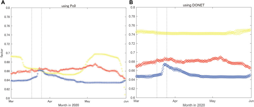
FIGURE 3. Time series of factor α for successive intervals of 12.42 h at C0002 (blue), C0010 (red), and C0006 (yellow). The reference pressures on the seafloor are assumed to be (A) Pc0 and (B) the nearest DONET station (KMD16 for C0002; KMD13 for C0010; KMC11 for C0006), respectively. Two vertical lines indicate the onset and termination time of the SSE that occurred in March 2020.
For C0010, the time function of α appears relatively stable before, during, and after the SSE. For C0006, where pore pressure change is expected to be negligible due to the SSE (Ariyoshi et al., 2021), it is quite stable in case of raw data of nearby DONET station and fluctuates in case of Pc0_raw for the reference seafloor pressure.
From these results, we conclude that the apparent increase of pore pressure at C0006 in Figure 2 is due to the instrumental drift at Pc0_raw, and that the instability as seen in Figure 2A at C0010 is not due to the malfunction of the reference pressure.
Figure 4 shows the time series of time lag (t0), where we apply the same operation to theoretical tide calculated by NAO.99Jb (Matsumoto et al., 2000) as shown in Figure 4B. Figures 5A–F show the histogram of frequency distribution for the time lag corresponding to Figure 4, and Figures 5G–I show the same histogram for the theoretical tidal component between boreholes and nearby DONET stations as shown in Figure 4B. As shown in Figure 4B and Figures 5G–I, time lag for the observation at nearby DONET station is greater than that for the theoretical one. This is because the pressure propagation of sea surface height change to the seafloor takes several seconds with decay due to baroclinic condition (e.g., Varlamov et al., 2015).
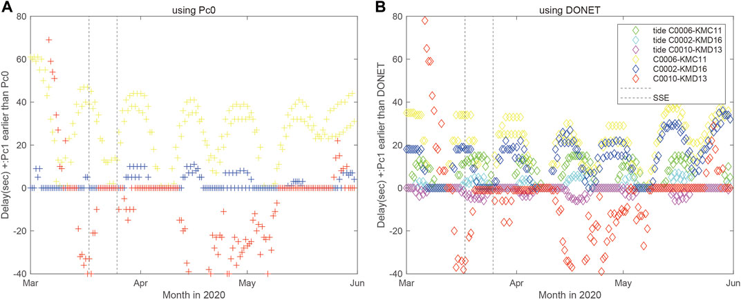
FIGURE 4. Time series of time lag t0, where t0 > 0 means Pc1_raw is earlier than the reference of raw data for (A) Pc0 and (B) PDONET_raw, respectively. Green colored plot in (B) shows the time lag of pressure change on the seafloor on the basis of theoretical tide between C0006 and KMC11. The others are the same as Figure 3.
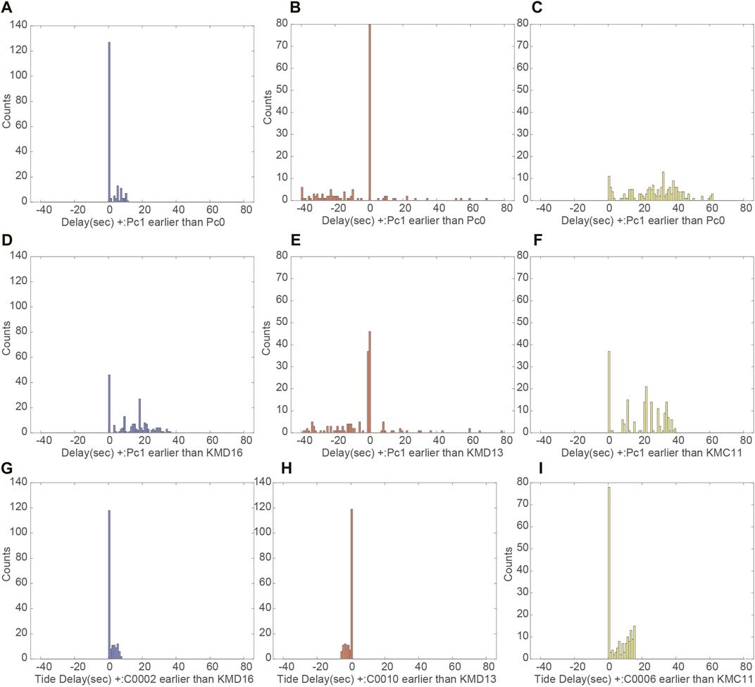
FIGURE 5. Frequency distribution histograms of the time lag t0 between raw data of Pc1 and the reference seafloor pressure: Pc0 at (A) C0002, (B) C0010, (C) C0006, (D–F) PDONET_raw; (D) KMD16, (E) KMD13, (F) KMC11, (G–I) expected from theoretical tidal component between boreholes and nearby DONET stations: (G) C0002-KMD16, (H) C0010-KMD13, and (I) C0006-KMC11, respectively.
From Figure 4B and Figures 5D–F, time lag between Pc1_raw at C0006 and raw data of nearby DONET station KMC11 has a periodic change similar to the theoretical tidal component with smaller amplitude and time delay. This feature is also applicable for C0002 and C0010 whose sense of the time lag is consistent with the theoretical component as shown in Figures 5G,H. In Figures 5G–I, time lag is negative for C0010 (Figure 5H) while the other is positive (Figures 5G,I). This is because KMD13 locates eastward from C0010 and is triggered tidal force earlier.
From Figure 4A and Figures 5A–C, the estimation of time lag between raw data of Pc1 and Pc0 is mostly zero for C0002 and C0010, whereas it fluctuates for C0006 because the operation of cross correlation does not work well due to the decrease drift for Pc0_raw (Figure 2B). These results suggest that time lag between raw data of Pc1 and Pc0 is basically negligible for C0002 and C0010 while highly variable for C0006 because the drastic increase after May 2020 is larger than its tidal component.
In this section, we apply some patterns of α and t0 fixed for the entire period of data. As described in Temporal change of α during the SSE and its stability before and after the SSE and Relationship between temporal change of t0 and tidal perturbation sections, the estimated values of α and t0 at C0002 are affected by SSE and at all boreholes by the tidal component. From the time lag between raw data of Pc1 at C0006 and KMC11 in Figure 4B, there is time lag between observation (yellow) and theoretical tide (green) with periodic oscillations that are much longer than M2 tide component. This means that the assumption that tidal effects are negligible for the estimation of α and t0 is incorrect and these parameters do not vary in accordance with the theoretical tidal calculation.
Figure 6 shows time series of residual (L1 norm) and cross correlation coefficient with their scatter diagram. Figure 6C shows negatively correlation between residual and cross correlation coefficient. This means that the order of determination for α and t0 does not affect the best solution. Figures 6A,B show residual and cross correlation became larger and smaller during the SSE. This implies that it is reasonable to find the fixed parameters so that time window does not include the duration time of SSE. From these results, we adopt the fixed parameters α and t0 when the residual is the lowest by the fine search for each reference setting. The obtained values are listed in Table 1. Here, we adopt L1 norm which can reduce the effect of spike change due to local earthquakes (Ariyoshi et al., 2021), but the results are the same as L2 norm except Pc1 for C0006.
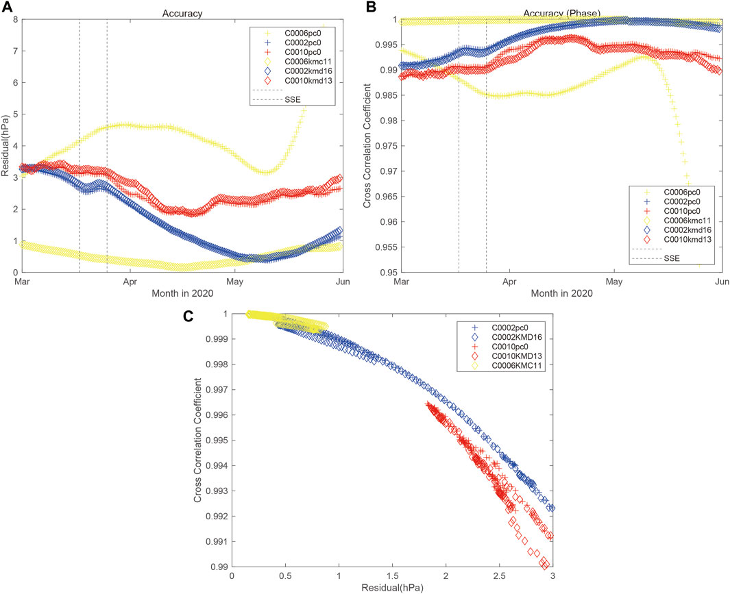
FIGURE 6. (A,B) Time series of (A) residual (L1 norm) and (B) cross correlation coefficient for each case. The others are the same as Figure 3. (C) Scatter diagram between (A) residual and (B) cross correlation coefficient.
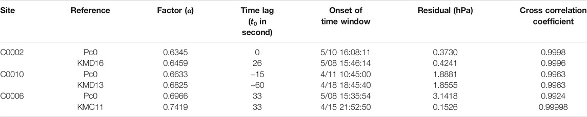
TABLE 1. Estimated parameters for estimation of pore pressure at Pc1.
Figure 7 shows the time series of pore pressure with the fixed parameters in Table 1 in case that the reference pressure on the seafloor is assumed as Pc0 and PDONET_raw. From Figure 7B, we find that the apparent increase of pore pressure at C0006 is removed by substituting Pc0_raw to KMC11 as the reference, while time lag between raw data of Pc1 and Pc0 at C0006 cannot cancel out the tidal component in Figure 7A. For the overall of C0002 and C0010, the pore pressure aligned by Pc0_raw is similar to that aligned by raw data of nearby DONET stations.
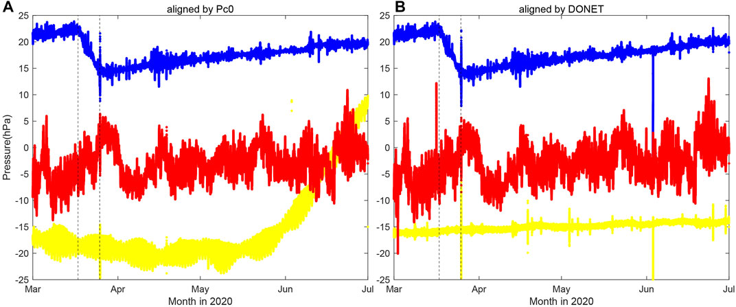
FIGURE 7. Time history of pore pressure in case of reference seafloor pressure treated as (A) Pc0 and (B) PDONET_raw with the fixed parameters in Table 1. The others are the same as Figure 2.
Figure 8 shows the amplitude spectrum of the pore pressure at Pc1 for each borehole station, focusing on M2 (12.42 h) and S2 (12 h) tides. For C0002, tidal component of M2 is removed by 30–40% for both Pc0 and KMD16 while S2 is increased by 20% for Pc0. These results suggest that the combination of M2 and S2 are totally decreased about 10–20%. For C0010, tidal component is removed by 10–30% for both of Pc0 and KMD13. Considering that the amplitude around M2 and S2 tides (0.52 and 0.5 days) is a significantly large peak, we think that the fluctuation at C0010 in Figure 2 and Figure 7 is excited by tidal components with non-linear time lag possibly due to failure of packing water in Figure 1C. For C0006, tidal component is removed by 60–90% for KMC11.
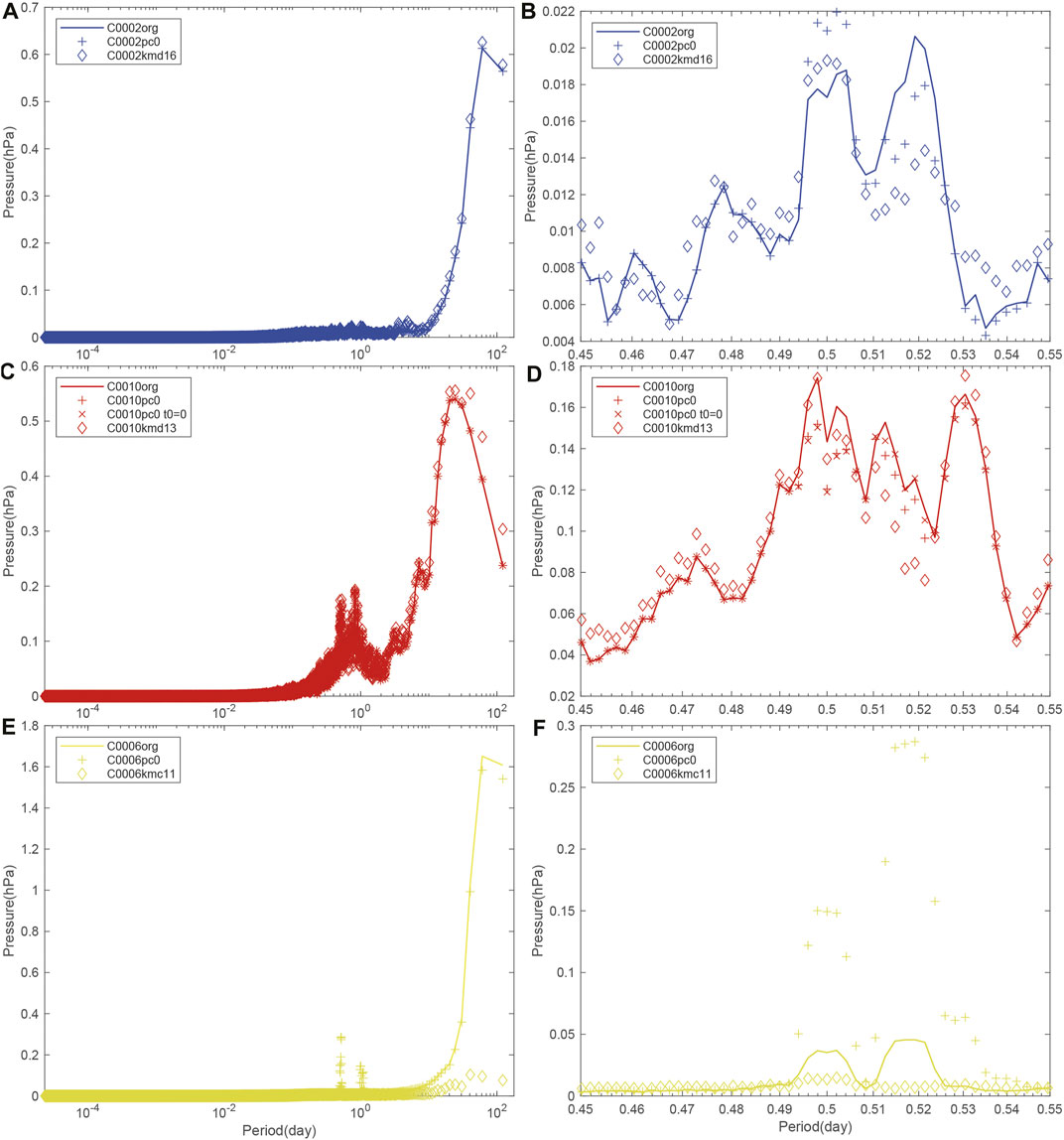
FIGURE 8. (A,C,E) Amplitude spectrum of pore pressure at Pc1_Pp at each borehole, (B,D,F) focusing on M2 and S2 tides, compared with Figure 2 (org). For C0010, Pc0 with t0 = 0 is additionally plotted.
Toward monitoring of pore pressure in real time, we determine the fixed value of α and t0 under the present condition. From the values of minimum residual and maximum cross correlation coefficient in Table 1, the reference pressure at C0002 and C0006 should be Pc0 and KMC11, respectively. For C0010, the values of the residual and cross correlation coefficient seem almost the same between Pc0 and KMD13. In addition, both of time lag (t0 = −15 and −60 s) is out of mode, average and median values as shown in Figure 5E. This indicates that the parameter values at C0010 in Table 1 might be determined by chance. To investigate the robustness, we also plot the amplitude spectrum in case of Pc0 without time lag (t0 = 0) in Figures 8cd, which shows that there seems no significant difference from the case with time lag. Therefore, it might be practical not to apply time lag in case of Pc0 at C0010, which is the same as the best condition for C0002.
Applying KMC11 to the reference seafloor pressure, we get the pore pressure at C0006 with high quality as demonstrated by Figure 7B and Table 1. Using this result, we discuss the crustal deformation there more detail. Figure 9 shows the close up of pore pressure history at C0006 before and after the SSE occurred in March 2020, which shows there exists compression about 0.6 hPa during the SSE. Considering that the onset and termination of the pore pressure change at C0006 is consistent with the duration time of the SSE determined from the pore pressure change at C0002 (Ariyoshi et al., 2021), we assume that this increase is due to crustal deformation driven by the SSE. Giving the conversion factor of C0006 as 5.0–6.0 kPa/μstrain (Davis et al., 2013; Araki et al., 2017; Ariyoshi et al., 2021), we roughly estimate the volumetric strain as 0.01 μstrain. This amount is about 10 times greater than expectation (0.0012 μstrain) from the fault model derived by Ariyoshi et al. (2021).
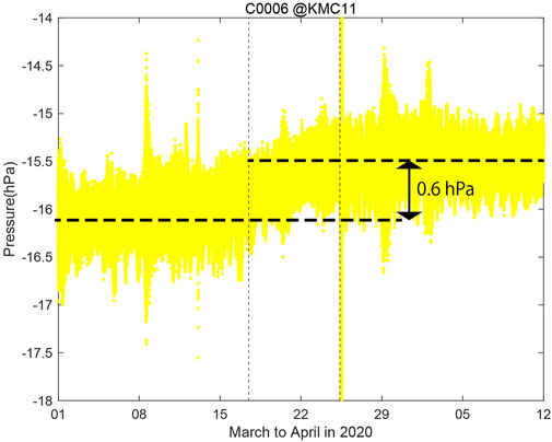
FIGURE 9. Close up of pore pressure history at C0006 before and after the SSE in March 2020 by applying KMC11 to the reference seafloor pressure. Vertical double arrows represent change amount during the SSE.
Considering the plate bending near the Nankai Trough as shown in Figure 1B and obtained dip angles of focal mechanism for the sVLFE in Figure 1A are in the range of 0–6°, we think that this discrepancy of the volumetric strain amount is mainly due to lower dip angle than the fault models (A-1 and A-2+ in Figure 1B) estimated by Ariyoshi et al. (2021), which assumes a planar fault dipping constantly at 6°.
To roughly estimate the valid dip angles for A-1 and A-2+ models, we calculate the volumetric strain change for dip angle in the range of 6–0° for A-2+ model with the same fault size, slip amount and strike angle as the original ones [fault geometry is listed in Table 5 of Ariyoshi et al. (2021)] by using a simple rectangular fault model (Okada, 1992) in a homogeneous elastic medium with a Poisson’s ratio of 0.35 (Araki et al., 2017) and a rigidity of 20 GPa. The result shows that the volumetric strain at C0002 due to the fault model of A-1 is nearly constant (0.001 μstrain) and largely independent of its dip angle. Hereafter, we focus on A-2+ model because the dip angle lower than 6° for the shallower fault (A-2+ model) is more reasonable than that for the deeper fault (A-1 model).
Table 2 and Figure 10 shows the volumetric strain changes of Pc1 at three boreholes as a function of dip angle for A-2+ model in Figure 1A. If the dip angle of A-2+ is treated as 6°, the volumetric strain at C0006 is slightly negative, which is inconsistent with the sense of the observational result (+0.01 μstrain) in Figure 9. If we adopt the reasonable range of the volumetric strain change at C0006 (vertical axis) as between 0.006 and 0.014 in Figure 10 (vertical axis), this result suggests that possible dipping angle of A-2+ is lower than 4°, which is largely consistent with the volumetric strain changes at C0002 (−0.074 μstrain) and C0010 (−0.22 μstrain) (Ariyoshi et al., 2021) by applying 5.7 and 4.7 kPa/μstrain, respectively (Davis et al., 2009; Wallace et al., 2016; Araki et al., 2017). This result is just a simplified interpretation and the unified fault model is to be proposed in our future study.
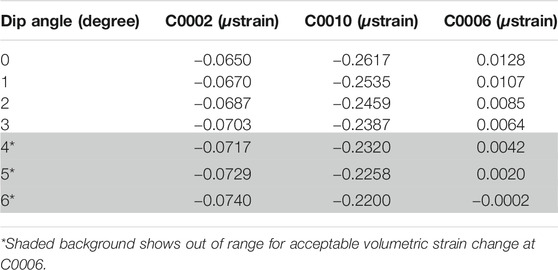
TABLE 2. Volumetric Strain as a function of dip angle for the fault model A-2.
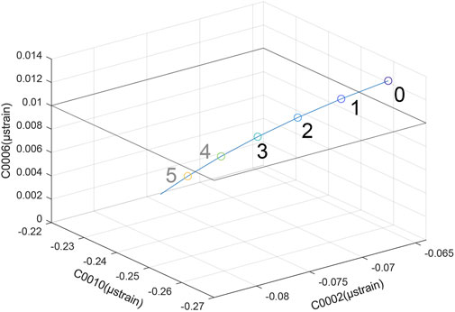
FIGURE 10. 3-D view of volumetric strain changes for Pc1 at three boreholes as a function of dip angle in degree (numerals) for the fault model A-2+ in Figure 1. Dip angle at 6° is slightly out of range (−0.0002 for vertical axis). Gray colored numbers (4, 5) indicate out of acceptable range.
To detect SSEs from pore pressure recorded in real time, it is important to distinguish oceanic perturbation from crustal deformation and understand the relationship between them. Gomberg et al. (2020) pointed out that ocean-pressure fluctuations on timescales longer than ∼5 days may affect only the termination and not the initiation of SSEs in the Hikurangi subduction zone. Since the relationship between termination time and ocean fluctuation has not been investigated yet at the Nankai Trough, we discuss it in the context of our results focusing on the SSE in March 2020.
To examine this suggestion, we calculate pressure fluctuations of the ocean variation on the seafloor at 1-h intervals by integrating the seawater density based on JCOPE ocean data assimilation system (JCOPE-T DA) (Miyazawa et al., 2021) from the sea surface to the seafloor and adding atmospheric sea level pressure. Note that tidal fluctuations on timescales shorter than ∼5 days are not accounted in the assimilation system. Another advantage of using JCOPE-T DA is the fact that the observed seafloor pressure data detided by the theoretical tide has still fluctuation about ±5 hPa and seems not reflect well baroclinic responses driven by Kuroshio meander (Matsumoto et al., 2021).
Figure 11 shows the time history of pressure fluctuated by ocean loading and pore pressures at Pc1 in each borehole by applying (Pc0, Pc0, KMC11) to the reference seafloor pressure at (C0002, C0010, C0006), respectively, with a time lag between the variations at C0006 and KMC11 listed in Table 1. To eliminate the tidal effect possibly included in the pressure fluctuation of the JCOPE-T DA, we adopt moving average for 25 h as shown by curves in Figure 11A. All the time histories of the moving average seem to represent short-term (about 5 days) oscillation. On the termination of the SSE, considering that fault regions of models A-1 and A-2+ cover under the boreholes at C0002 and C0010 (Figure 1), we find that their short-term oscillations are in increase phase. The amplitude of the short-term oscillation at C0002 and C0010 on the termination of SSE is about 6 hPa, which is consistent with statistically significance for pressure distributions at the SSEs in the Hikurangi as shown by Figure 3 of Gomberg et al. (2020). For C0006, Figure 11A shows the short-term oscillation is in increase phase with small amplitude (1∼3 hPa).
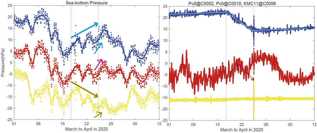
FIGURE 11. (A) Time history of detided pressure changes integrated from atmosphere to seafloor on the basis of JCOPE-T DA with the same colors as Figure 2A. Bold curves show moving average for 25 h. Vertical lines show the onset and termination time of the SSE in March 2020. Long and short arrows represent the trend change between the onset and termination of the SSE and short-term oscillation at the termination of the SSE. (B) Time history of pore pressure for corresponding time span. Dotted arrows show the crustal deformation component of pore pressure on the basis of models A-1 and A-2+ estimated by Ariyoshi et al. (2021). Light cyan lines show the regression analysis estimated by Ariyoshi et al. (2021).
Gomberg et al. (2020) suggested the physical relationship between the ocean loading and the SSE termination (in Figure 5 of their paper). The ocean loading affects the termination of the SSE as well as initiation when the fault slip causes temporal weakening of the fault strength. The fault strength is thought to depend on the time history of slip velocity and shear/normal stress in addition to frictional properties (e.g., Yoshida et al., 2020) perturbed by the SSE. In order to estimate the time history of the fault strength, it is necessary to know the time history of detailed slip process in realistic model of the SSE as well as the frictional properties, which is our future work.
The seafloor pressure changes between the onset and termination of the SSE as indicated by long arrows in Figure 11A seem to be negatively correlated with the pore pressure change in Figure 11, particularly clear for C0002 (∼+6 hPa) and C0006 (∼−6 hPa). For C0002, the pore pressure change seems to be fitted as a ramp function, which is similar to the previous SSE in 2015 (Araki et al., 2017). By applying regression analysis, we estimate the time history of crustal deformation as shown by light cyan lines. For C0010, it is difficult to find the negative correlation because the crustal deformation component of the pore pressure is complicated due to the passage of fault slip by models A-1 to A-2+ in Figure 1A, which is statistically estimated by Ariyoshi et al. (2021) as shown by arrows in Figure 11B.
During the SSE in March 2020, a Kuroshio meander occurred around DONET stations. To trace the Kuroshio meander and to monitor the deep thermal structure of the cold (higher density) core eddy south of Enshu-nada, we investigate the distributions in water temperatures at depths of 200 and 600 m (Figure 12), respectively. Associated with a westward movement of the current path of the Kuroshio indicated by the 15°C isotherm at a 200 m depth, a warm (lower density) water mass proceeded from the east of C0006 to near C0002 (Figures 12A–C). Meanwhile, at a 600 m depth, the deep cold water mass beneath the cold eddy off Enshu-nada propagated northward (Figures 12D–F).
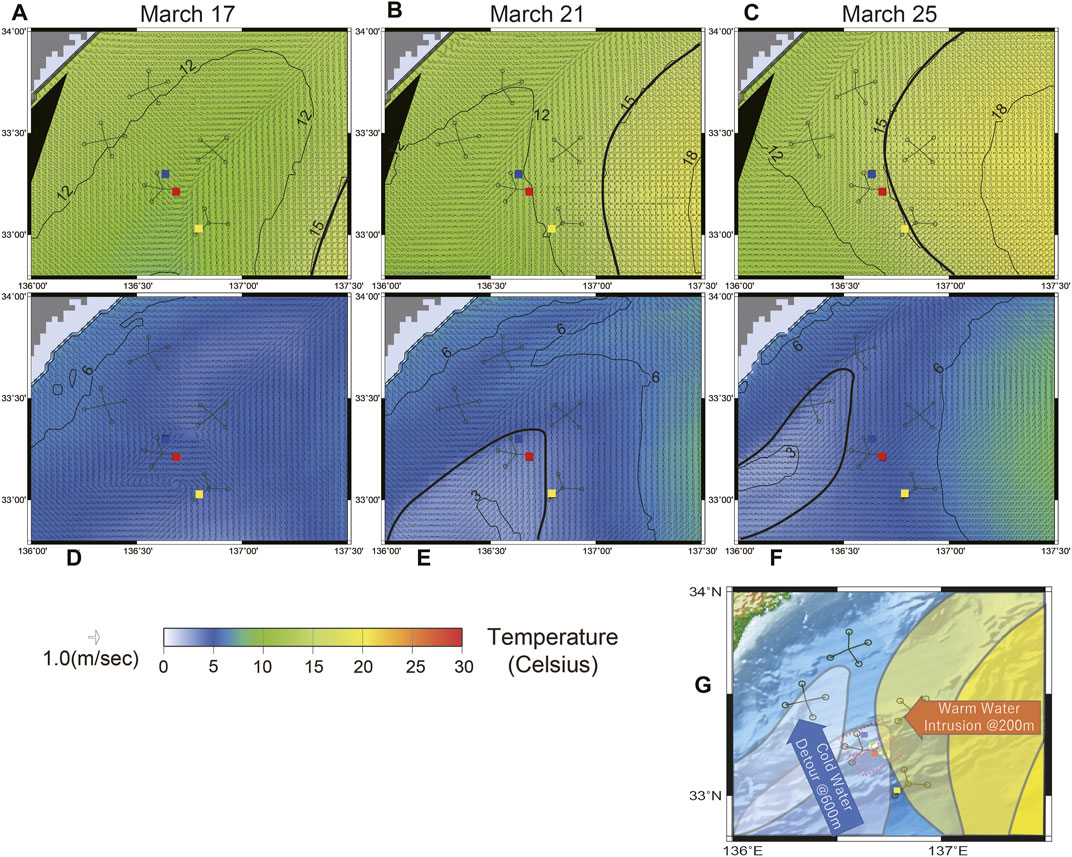
FIGURE 12. Ocean temperature with current vector at the depths of (A–C) 200 and (D–F) 600 m under the sea surface with isothermal contours (3°). Circles and squares represent DONET and borehole stations, respectively. (G) Schematic illustration of the S-shaped meandering pattern by tracing isothermal contours of 15 and 4° at the depths of 200 and 600 m as shown by bold curves in (A–F). Target region is the same as Figure 1A.
This feature is typically known as S-shaped meandering pattern (Figure 13 of Kasai et al., 1993). It is well known that the Kuroshio front variability includes 5–8, and 10–12 days periodic fluctuations (Kimura and Sugimoto 1993), and 20–50 days fluctuations as S-shaped meander (Kasai et al., 1993; Miyama and Miyazawa 2014), where the transition between warm water intrusion and cold water detour seems S-shaped (Figure 12G). The seafloor pressure changes (Eq. 4) are consistent with the variations of water density changes associated with those in temperature (the third term of the right-hand side of Eq. 4), and contributions from the other terms (the first and second terms of the right-hand of Eq. 4) are negligible. The density changes induced by the movement of the cold water are more evident at C0002 and C0010 than at C0006 (Figure 12).
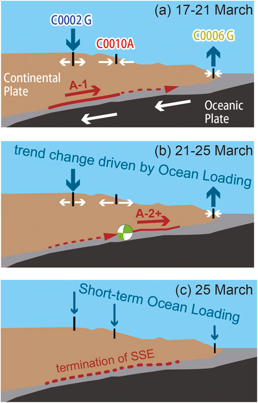
FIGURE 13. Schematic scenario of the possible process for the SSE with ocean loading (A) during model A-1, (B) during model A-2+, and (C) termination of the SSE. Representative focal mechanism of VLFE is obtained from Ariyoshi et al. (2021). Double arrows represent volumetric strain change due to crustal deformation driven by the SSE.
Since less normal stress on the fault promotes slip generation on the basis of Coulomb Failure Stress (CFS) (= τ + μ(σ-P), where τ is shear stress, μ is friction, σ is normal stress, P is pore pressure) (e.g., Labuz and Zang, 2012), we discuss the possibility of SSE triggered by ocean fluctuation quantitatively. According to Kanamori and Anderson (1975), stress drop is obtained as
where Δτ is the stress drop, G is the rigidity, D is the slip amount on the fault, W is the fault width. For model A-2+, Δτ is estimated as 24 kPa, where G is treated as 20 GPa. Neglecting dip angle (<4°), we can roughly estimate ΔCFS [=μ(Δσ), where we neglect dip angle <4°] as 2∼3 hPa, which is about 1% of the stress drop.
From theoretical research, static stress change is more effective to trigger fault slip than dynamic stress perturbation (e.g., Gomberg et al., 1998). Yoshida et al. (2020) performed a numerical simulation of earthquake cycle on the basis of rate- and state-friction laws on a simplified subduction plate boundary. With static and dynamic change of effective normal stress 1/8 time of recurrence interval before the earthquake onset, earthquakes can be instantaneously triggered by static change of less than 2.5% of stress drop while not by dynamic change of greater than 8% of stress drop. If we assume that the frictional state on the fault model A-2+ as the condition ready to occur fault slip due to nearby slip on the fault model A-1, and that the trend change is approximately applicable to static change, the amount of pressure for the trend change could be sufficient to promote slip upward through the source regions of sVLFEs.
Focusing on the pressure change around the termination of the SSE in Figure 11B (Supplementary Figure S1), impulsive pore pressure change occurs all the three borehole stations. This is thought to be excited by seismic waves of the March 25, 2020 Mw7.5 earthquake in northern Kuril Island (Ye et al., 2021). The arrival time of the P-wave is estimated as 298 s later after the origin time (11:49:21 in JST + 9 h from UTC) from tauP (Crotwell et al., 1999), which seems consistent with the arrival time at KMD13 (11:54:19) and later than the SSE termination time at around 08:40 in JST (Supplementary Figure S1).
Since the standard deviation of the estimated SSE onset/termination time is 9 h (Ariyoshi et al., 2021), it might be possible that the seismic waves also affect the termination. Since the previous studies focused on the clock advance of triggering earthquakes (Gomberg et al., 1998; Yoshida et al., 2020), it is necessary to investigate the clock advance of terminating earthquakes, which is our future study.
Figure 13 shows a schematic explanation about the possible scenario of the SSE in March 2020. The trend change driven by oceanic fluctuation (Figures 13A,B) promotes shallower slip causing sVLFEs during the passage of Kuroshio meander, and increase of normal stress due to the short-term oscillation (Figure 13C) promotes termination of the SSE as observed in the Hikurangi subduction. Therefore, monitoring of oceanic oscillation especially ocean current meander is also important to forecast the growth of SSE and avoid the misdetection of crustal deformation.
Because JCOPE-T DA is the latest version of JCOPE (Miyazawa et al., 2021), it costs much time to get the reanalyzed ocean modeling going back from the present to past time. It is our future work to apply JCOPE-T DA to the time when previous SSEs occurred, which would reveal more detailed relationship between Kuroshio meander and previous SSEs.
Our conclusions are summarized as follows.
i) If we use the reference pressure on the seafloor just above the borehole, time lag is negligible for one second sampling. This shows we can monitor pore pressure simply by subtracting the reference pressure with valid factor if the instrumental drift component is negligible.
ii) We demonstrate that the reference seafloor pressures at boreholes can be substituted with nearby DONET seafloor pressure gauge data. This would give more robust condition to monitor the pore pressure in case of malfunctioning of the borehole reference pressure gauge.
iii) The time lag of the pressure between borehole and nearby DONET station is temporarily perturbed due to tidal oscillation, which can be explained by superposition of tidal modes. The amplification factor of the reference seafloor pressure to borehole pressure is perturbed during the occurrence of nearby SSE in case of significant pore pressure change.
iv) Using the seafloor pressures recorded at the nearby DONET station to the borehole pressures at C0006, we can extract the pore pressure change due to crustal deformation of the SSE in March 2020 at the deepest borehole (Pc1) of C0006 about 0.6 hPa.
v) On the basis of ocean modeling, the ocean impact of seafloor pressure without tidal effect has short-term (5 days) oscillation and trend change between the onset and termination of the SSE. The amount of ΔCFS around C0006 is about several percent of stress drop for the SSE, which may be sufficient to promote updip slip propagation toward the fault model which triggered sVLFEs.
In summary, real-time monitoring of precise pore pressure with nearby DONET stations and ocean modeling would be a powerful tool to judge the onset and termination of SSEs promptly.
Borehole data is available from the website of the J-SEIS (JAMSTEC Ocean-bottom Seismology Database; https://join-web.jamstec.go.jp/join-portal/). DONET data is available from the website of NIED (National Research Institute for Earth Science and Disaster Resilience) https://doi.org/10.17598/nied.0008. The JCOPE-T DA data are available from the website of JAMSTEC; http://www.jamstec.go.jp/jcope/htdocs/e/distribution/.
KA estimated the best solution of the factors and time delays between boreholes and nearby DONET station, in addition to write the manuscript overall. TK tested the application of nearby DONET seafloor pressure data. YM wrote Ocean model product used for calculation of atmosphere-ocean-induced sea floor pressure fluctuations section. SV customized the JCOPE-T DA for boreholes and DONET stations. TI calculate the dependency of the volumetric strain on the dip angle in Figure 10. AN revised Oceanic fluctuation impact on the seafloor section. JG revised the manuscript as a native English writer. EA designed the borehole and DONET observatories. TM advised the interpretation of the results from JCOPE-T DA. KS managed the borehole and DONET data server. SY supported for making Figure 13. TH and SK coordinated the research discussion. NT managed the data sharing of DONET.
This work was partly supported by the Japan Society for the Promotion of Sciences (JSPS), Grant-in-Aid for Scientific Research (KAKENHI) Grant Numbers JP20H02236 and JP20KK0097.
The authors declare that the research was conducted in the absence of any commercial or financial relationships that could be construed as a potential conflict of interest.
All claims expressed in this article are solely those of the authors and do not necessarily represent those of their affiliated organizations, or those of the publisher, the editors and the reviewers. Any product that may be evaluated in this article, or claim that may be made by its manufacturer, is not guaranteed or endorsed by the publisher.
tGeneric Mapping Tools (Wessel et al., 2013) was used to create figures. Figure 13 was revised from PR section of JAMSTEC. The authors would like to thank H. Matsumoto and Jeff McGuire for their fruitful discussion and review. The authors would like to thank K. Hisamatsu for kindly providing a schematic illustration based on Figure 13. The authors would like to thank the Editorial Office of Frontiers in Earth Science to encourage our submission.
The Supplementary Material for this article can be found online at: https://www.frontiersin.org/articles/10.3389/feart.2021.717696/full#supplementary-material
Supplementary Figure S1 | Close up of Figure 11B showing the time history of pore pressure at C0002 (blue), C0010 (red), and C0006 (yellow) with regression lines (light cyan and magenta) before and after the SSE. Time is set to JST (+9hours from UTC).
Annoura, S., Hashimoto, T., Kamaya, N., and Katsumata, A. (2017). Shallow Episodic Tremor Near the Nankai Trough axis off Southeast Mie Prefecture, Japan. Geophys. Res. Lett. 44, 3564–3571. doi:10.1002/2017GL073006
Aoi, S., Asano, Y., Kunugi, T., Kimura, T., Uehira, K., Takahashi, N., et al. (2020). MOWLAS: NIED Observation Network for Earthquake, Tsunami and Volcano. Earth Planets Space 72, 126. doi:10.1186/s40623-020-01250-x
Araki, E., Saffer, D. M., Kopf, A. J., Wallace, L. M., Kimura, T., Machida, Y., et al. (2017). Recurring and Triggered Slow-Slip Events Near the Trench at the Nankai Trough Subduction Megathrust. Science 356, 1157–1160. doi:10.1126/science.aan3120
Ariyoshi, K., Iinuma, T., Nakano, M., Kimura, T., Araki, E., Machida, Y., et al. (2021). Characteristics of Slow Slip Event in March 2020 Revealed from Borehole and DONET Observatories. Front. Earth Sci. 8, 600793. doi:10.3389/feart.2020.600793
Ariyoshi, K., Nakata, R., Matsuzawa, T., Hino, R., Hori, T., Hasegawa, A., et al. (2014). The Detectability of Shallow Slow Earthquakes by the Dense Oceanfloor Network System for Earthquakes and Tsunamis (DONET) in Tonankai District, Japan. Mar. Geophys. Res. 35, 295–310. doi:10.1007/s11001-013-9192-6
Crotwell, H. P., Owens, T. J., and Ritsema, J. (1999). The TauP Toolkit: Flexible Seismic Travel-Time and ray-path Utilities. Seismological Res. Lett. 70, 154–160. doi:10.1785/gssrl.70.2.154
Davis, E., Becker, K., Wang, K., and Kinoshita, M. (2009). Co-seismic and post-seismic Pore-Fluid Pressure Changes in the Philippine Sea Plate and Nankai Decollement in Response to a Seismogenic Strain Event off Kii Peninsula, Japan. Earth Planet. Sp 61, 649–657. doi:10.1186/bf03353174
Davis, E., Kinoshita, M., Becker, K., Wang, K., Asano, Y., and Ito, Y. (2013). Episodic Deformation and Inferred Slow Slip at the Nankai Subduction Zone during the First Decade of CORK Borehole Pressure and VLFE Monitoring. Earth Planet. Sci. Lett. 368, 110–118. doi:10.1016/j.epsl.2013.03.009
Dragert, H., Wang, K., and James, T. S. (2001). A Silent Slip Event on the Deeper Cascadia Subduction Interface. Science 292, 1525–1528. doi:10.1126/science.1060152
Egbert, G. D., and Erofeeva, S. Y. (2002). Efficient Inverse Modeling of Barotropic Ocean Tides. J. Atmos. Oceanic Technol. 19, 183–204. doi:10.1175/1520-0426(2002)019<0183:eimobo>2.0.co;2
Gomberg, J., Baxter, P., Smith, E., Ariyoshi, K., and Chiswell, S. M. (2020). The Ocean's Impact on Slow Slip Events. Geophys. Res. Lett. 47, e2020GL087273. doi:10.1029/2020GL087273
Gomberg, J., Beeler, N. M., Blanpied, M. L., and Bodin, P. (1998). Earthquake Triggering by Transient and Static Deformations. J. Geophys. Res. 103 (B10), 24411–24426. doi:10.1029/98JB01125
Ide, S., Beroza, G. C., Shelly, D. R., and Uchide, T. (2007). A Scaling Law for Slow Earthquakes. Nature 447, 76–79. doi:10.1038/nature05780
Ito, Y., Obara, K., Shiomi, K., Sekine, S., and Hirose, H. (2007). Slow Earthquakes Coincident with Episodic Tremors and Slow Slip Events. Science 315, 503–506. doi:10.1126/science.1134454
Kanamori, H., and Anderson, D. L. (1975). Theoretical Basis of Some Empirical Relations in Seismology. Bull. Seismological Soc. America 65, 1073–1095.
Kaneda, Y., Kawaguchi, K., Araki, E., Matsumoto, H., Nakamura, T., Kamiya, S., et al. (2015). in Development and Application of an Advanced Ocean Floor Network System for Megathrust Earthquakes and Tsunamis. Editor P. Favali (Springer Praxis Books), 643–662. doi:10.1007/978-3-642-11374-1_25
Kasai, A., Kimura, S., and Sugimoto, T. (1993). Warm Water Intrusion from the Kuroshio into the Coastal Areas South of Japan. J. Oceanogr 49, 607–624. doi:10.1007/bf02276747
Kawaguchi, K., Kaneko, S., Nishida, T., Komine, T., et al. (2015). “Construction of the DONET Real-Time Seafloor Observatory for Earthquakes and Tsunami Monitoring,”. Editor P. Favali (Springer Praxis Books), 211–228. doi:10.1007/978-3-642-11374-1_10
Kimura, S., and Sugimoto, T. (1993). Short-period Fluctuations in Meander of the Kuroshio's Path off Cape Shiono Misaki. J. Geophys. Res. 98 (C2), 2407–2418. doi:10.1029/92jc02582
Kinoshita, M., Becker, K., Toczko, S., Edgington, J., Kimura, T., Machida, Y., et al. (2018). “Expedition 380 Methods,” in The Expedition 380 Scientists, NanTroSEIZE Stage 3: Frontal Thrust Long-Term Borehole Monitoring System (LTBMS). Proceedings of the International Ocean Discovery Program. Editors K. Becker, M. Kinoshita, and S. Toczko (College Station, TX: International Ocean Discovery Program)), 380. doi:10.14379/iodp.proc.380.102.2018
Labuz, J. F., and Zang, A. (2012). Mohr-Coulomb Failure Criterion. Rock Mech. Rock Eng. 45, 975–979. doi:10.1007/s00603-012-0281-7
Machida, Y., Araki, E., Nishida, S., Kimura, T., and Matsumoto, H. (2019). On the Accuracy of Quartz Pressure Sensor in the Seafloor Affected by Transport Condition. IEEE J. Oceanic Eng. 44, 1049–1057. doi:10.1109/JOE.2018.2855478
Matsumoto, H., and Araki, E. (2021). Drift Characteristics of DONET Pressure Sensors Determined from In-Situ and Experimental Measurements. Front. Earth Sci. 8, 600966. doi:10.3389/feart.2020.600966
Matsumoto, H., Nagano, A., Ariyoshi, K., and Araki, E., (2021). Effect of Ocean Current on Long-Term In-Situ Pressure Observation in Sagami Bay. Tokyo: Proceedings of Japan Society of Civil Engineers. Accepted. (written in Japanese with English abstract).
Matsumoto, K., Takanezawa, T., and Ooe, M. (2000). Ocean Tide Models Developed by Assimilating TOPEX/POSEIDON Altimeter Data into Hydrodynamical Model: A Global Model and a Regional Model Around Japan. J. Oceanography 56, 567–581. doi:10.1023/a:1011157212596
Matsuzawa, T., Hirose, H., Shibazaki, B., and Obara, K. (2010). Modeling Short- and Long-Term Slow Slip Events in the Seismic Cycles of Large Subduction Earthquakes. J. Geophys. Res. 115, B12301. doi:10.1029/2010JB007566
Miyama, T., and Miyazawa, Y. (2014). Short-term Fluctuations South of Japan and Their Relationship with the Kuroshio Path: 8- to 36-day Fluctuations. Ocean Dyn. 64, 537–555. doi:10.1007/s10236-014-0701-1
Miyazawa, Y., Varlamov, S. M., Miyama, T., Kurihara, Y., Murakami, H., and Kachi, M. (2021). A Nowcast/Forecast System for Japan's Coasts Using Daily Assimilation of Remote Sensing and In Situ Data. Remote Sensing 13, 2431. doi:10.3390/rs13132431
Nakano, M., Hori, T., Araki, E., Kodaira, S., and Ide, S. (2018). Shallow Very-Low-Frequency Earthquakes Accompany Slow Slip Events in the Nankai Subduction Zone. Nat. Commun. 9, 984. doi:10.1038/s41467-018-03431-5
Nishikawa, T., Matsuzawa, T., Ohta, K., Uchida, N., Nishimura, T., and Ide, S. (2019). The Slow Earthquake Spectrum in the Japan Trench Illuminated by the S-Net Seafloor Observatories. Science 365, 808–813. doi:10.1126/science.aax5618
Obara, K., and Kato, A. (2016). Connecting Slow Earthquakes to Huge Earthquakes. Science 353, 253–257. doi:10.1126/science.aaf1512
Obara, K. (2002). Nonvolcanic Deep Tremor Associated with Subduction in Southwest Japan. Science 296, 1679–1681. doi:10.1126/science.1070378
Okada, Y. (1992). Internal Deformation Due to Shear and Tensile Faults in a Half-Space. Bull. Seismological Soc. America 82, 1018–1040.
Schwartz, S. Y., and Rokosky, J. M. (2007). Slow Slip Events and Seismic Tremor at Circum-Pacific Subduction Zones. Rev. Geophys. 45, a–n. doi:10.1029/2006RG000208
Shirahata, K., Yoshimoto, S., Tsuchihara, T., and Ishida, S. (2019). Study on Aquifer Hydraulic Properties Using Tidal Response Method for Future Groundwater Development. Paddy Water Environ. 17, 531–537. doi:10.1007/s10333-019-00749-8
Takagi, R., Uchida, N., and Obara, K. (2019). Along‐Strike Variation and Migration of Long‐Term Slow Slip Events in the Western Nankai Subduction Zone, Japan. J. Geophys. Res. Solid Earth 124, 3853–3880. doi:10.1029/2018JB016738
Takemura, S., Noda, A., Kubota, T., Asano, Y., Matsuzawa, T., and Shiomi, K. (2019). Migrations and Clusters of Shallow Very Low Frequency Earthquakes in the Regions Surrounding Shear Stress Accumulation Peaks along the Nankai Trough. Geophys. Res. Lett. 46, 11830–11840. doi:10.1029/2019GL084666
Tanaka, S., Matsuzawa, T., and Asano, Y. (2019). Shallow Low‐Frequency Tremor in the Northern Japan Trench Subduction Zone. Geophys. Res. Lett. 46, 5217–5224. doi:10.1029/2019GL082817
Varlamov, S. M., Guo, X., Miyama, T., Ichikawa, K., Waseda, T., and Miyazawa, Y. (2015). M2baroclinic Tide Variability Modulated by the Ocean Circulation South of Japan. J. Geophys. Res. Oceans 120, 3681–3710. doi:10.1002/2015JC010739
Wallace, L. M., Araki, E., Saffer, D., Wang, X., Roesner, A., Kopf, A., et al. (2016). Near‐field Observations of an Offshore M W 6.0 Earthquake from an Integrated Seafloor and Subseafloor Monitoring Network at the Nankai Trough, Southwest Japan. J. Geophys. Res. Solid Earth 121, 8338–8351. doi:10.1002/2016jb013417
Wessel, P., Smith, W. H. F., Scharroo, R., Luis, J., and Wobbe, F. (2013). Generic Mapping Tools: Improved Version Released, Eos Trans. AGU 95(45), 409.
Ye, L., Lay, T., and Kanamori, H. (2021). The 25 March 2020 M 7.5 Paramushir, Northern Kuril Islands Earthquake and Major (M ≥ 7.0) Near-Trench Intraplate Compressional Faulting. Earth Planet. Sci. Lett. 556, 116728. doi:10.1016/j.epsl.2020.116728
Keywords: slow slip event, slow earthquake, Kuroshio meander, Nankai Trough, ocean modeling
Citation: Ariyoshi K, Kimura T, Miyazawa Y, Varlamov S, Iinuma T, Nagano A, Gomberg J, Araki E, Miyama T, Sueki K, Yada S, Hori T, Takahashi N and Kodaira S (2021) Precise Monitoring of Pore Pressure at Boreholes Around Nankai Trough Toward Early Detecting Crustal Deformation. Front. Earth Sci. 9:717696. doi: 10.3389/feart.2021.717696
Received: 31 May 2021; Accepted: 22 July 2021;
Published: 27 August 2021.
Edited by:
Sergey V. Samsonov, Department of Natural Resources, CanadaCopyright © 2021 Ariyoshi, Kimura, Miyazawa, Varlamov, Iinuma, Nagano, Gomberg, Araki, Miyama, Sueki, Yada, Hori, Takahashi and Kodaira. This is an open-access article distributed under the terms of the Creative Commons Attribution License (CC BY). The use, distribution or reproduction in other forums is permitted, provided the original author(s) and the copyright owner(s) are credited and that the original publication in this journal is cited, in accordance with accepted academic practice. No use, distribution or reproduction is permitted which does not comply with these terms.
*Correspondence: Keisuke Ariyoshi, YXJpeW9zaGlAamFtc3RlYy5nby5qcA==
Disclaimer: All claims expressed in this article are solely those of the authors and do not necessarily represent those of their affiliated organizations, or those of the publisher, the editors and the reviewers. Any product that may be evaluated in this article or claim that may be made by its manufacturer is not guaranteed or endorsed by the publisher.
Research integrity at Frontiers
Learn more about the work of our research integrity team to safeguard the quality of each article we publish.