 Richard Fiifi Annan
 Xiaoyun Wan
- School of Land Science and Technology, China University of Geosciences (Beijing), Beijing, China
A regional gravity field product, comprising vertical deflections and gravity anomalies, of the Gulf of Guinea (15°W to 5°E, 4°S to 4°N) has been developed from sea surface heights (SSH) of five altimetry missions. Though the remove-restore technique was adopted, the deflections of the vertical were computed directly from the SSH without the influence of a global geopotential model. The north-component of vertical deflections was more accurate than the east-component by almost three times. Analysis of results showed each satellite can contribute almost equally in resolving the north-component. This is attributable to the nearly northern inclinations of the various satellites. However, Cryosat-2, Jason-1/GM, and SARAL/AltiKa contributed the most in resolving the east-component. We attribute this to the superior spatial resolution of Cryosat-2, the lower inclination of Jason-1/GM, and the high range accuracy of the Ka-band of SARAL/AltiKa. Weights of 0.687 and 0.313 were, respectively, assigned to the north and east components in order to minimize their non-uniform accuracy effect on the resultant gravity anomaly model. Histogram of computed gravity anomalies compared well with those from renowned models: DTU13, SIOv28, and EGM2008. It averagely deviates from the reference models by −0.33 mGal. Further assessment was done by comparing it with a quadratically adjusted shipborne free-air gravity anomalies. After some data cleaning, observations in shallow waters, as well as some ship tracks were still unreliable. By excluding the observations in shallow waters, the derived gravity field model compares well in ocean depths deeper than 2,000 m.
Introduction
The advancements in satellite altimetry since the past 4 decades has led to the proliferation of sea surface height (SSH) data which has contributed significantly to geodesy, geophysics, oceanography, and hydrology. Some of its applications include: sea level variation research (Cazenave et al., 2014; Ablain et al., 2015; Watson et al., 2015; Passaro et al., 2018), determination of mean dynamic topography (MDT) and mean sea surface (Andersen et al., 2016; Ophaug et al., 2021), construction of marine geoid (Dadzie and Li, 2007; Chander and Majumdar, 2016), monitoring of lakes and rivers (Villadsen et al., 2015; Zakharova et al., 2019) and inversion of marine gravity field (Sandwell et al., 2013; Sandwell et al., 2014; Zhu et al., 2019; Nguyen et al., 2020; Wan et al., 2020b).
Marine gravity anomaly is an important geophysical quantity with applications in marine resources exploration and exploitation (Becker et al., 2009), geoid modeling (Olgiati et al., 1995; Hwang, 1998; Soltanpour et al., 2007), delimitation of continent–ocean boundaries (Sandwell et al., 2013), revelation of submarine tectonic structures (Hwang and Chang, 2014; Sandwell et al., 2014; Wan et al., 2020a), and bathymetry augmentation (Hwang, 1999). Marine gravity anomaly can be inverted from geoid heights after SSH is reduced to geoid by the removal of dynamic sea surface topography (Olgiati et al., 1995; Andersen et al., 2010; Nguyen et al., 2020). It can also be derived from the deflection of the vertical, whereby the geoid heights are differenced along satellite orbits to obtain geoid gradients. The along-track geoid gradients are then converted to vertical deflections. This along-track differentiation has the advantage of reducing the impact of long wavelength errors (Hwang et al., 2002; Zhu et al., 2019). Also, the vertical deflections approach does not require crossover adjustment (Hwang et al., 2002).
Since marine surface phenomena mostly have submarine origins, with these submarine activities best revealed through gravity anomalies, it is imperative to derive accurate marine gravity models to aid in understanding marine phenomena. Since the past decade, there have been an increase in the quantity and quality of altimetry data, as well as superior computing hardware. This has led to various researchers to develop gravity field models for their respective countries and economic blocs. For instance: over the South China Sea, Zhang et al. (2017) and Zhu et al. (2020) separately developed 1′ × 1′ marine gravity models by amalgamating multi-satellite SSH data; Nguyen et al. (2020) merged gravity anomaly derived from Cryosat-2 and Saral/AltiKa SSH datasets with shipborne gravity data over the Gulf of Tonkin area of Vietnam. A recent study by Sandwell et al. (2013) has shown that gravity field models derived from modern altimeter satellites are more accurate than those obtained from some governmental shipborne gravity data. This shows the usefulness of satellite-derived gravity models in filling the gaps between tracks of shipborne gravimetry. It must be appreciated that though gravimetry via ships is still reliable, it is expensive, slow and mostly limited to the maritime waters of developed countries. Therefore, SSH datasets from altimetry satellites are the best and cheapest option for developing regions like West Africa.
It is expected that the development of the study region synchronizes with scientific investigations of its largest natural resource (the ocean); however, this is yet to be realised. Even though the region is oil-rich (Osaretin, 2011; Bazilian et al., 2013), the scantiness of reviewed literatures about the maritime waters of West Africa shows that the region’s maritime waters is one of the least studied. The study area encompasses 15°W to 5°E, and 4°S to 4°N. Countries of interest include Guinea and Guinea Bissau at the western end, through to the central-south African country of The Congo.
The present study aims to study the gravity field of the region by using vertical deflections derived from the geodetic missions (GM) of Jason-1, Saral/AltiKa, Haiyang-2A; Cryosat-2, and Envisat. We achieve this objective through the remove-restore procedure using EGM2008 as the reference gravity filed model. The use of EGM2008 is due to the fact that it is the most frequently used global geopotential model for marine geodetic and geophysical research (Andersen et al., 2010; Sandwell et al., 2014; Zhang et al., 2017; Andersen and Knudsen, 2019; Zhu et al., 2019; Zhu et al., 2020).
Materials and Methods
Altimetry Data
The altimetry datasets used in this research comprises GDR (geophysical data record) of eight cycles of Jason-1/GM, seven cycles of Saral/AltiKa, five cycles of Envisat, five cycles of Cryosat-2, and IGDR (interim geophysical data record) of seven cycles of HY-2A/GM. The Jason-1 GDRs were obtained from the Physical Oceanography Distributed Active Archive Center, Jet Propulsion Laboratory, NASA (https://podaac.jpl.nasa.gov/JASON1?sections=data). Saral/AltiKa GDRs were obtained from AVISO (https://www.aviso.altimetry.fr/), Envisat and Cryosat-2 GDRs were provided by the European Space Agency (http://earth.esa.int); while HY-2A GDRs were provided by the National Satellite Ocean Administration Service of China (ftp2.nsoas.org.cn). Along-track SSH is computed from each cycle as given by Eq. 1. Table 1 is a summary of the various selection criteria applied to each satellite’s dataset during SSH computation. Figure 1 shows the spatial distribution of ground tracks of the different satellites.
where
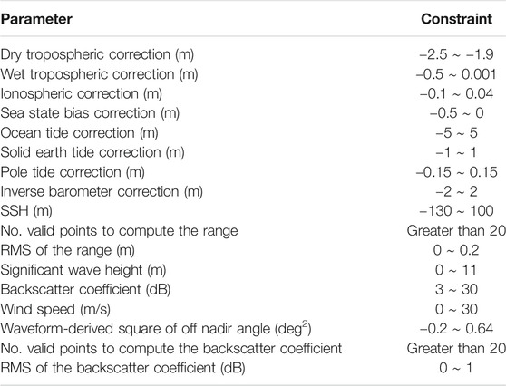
TABLE 1. Selection criteria for SSH computation.
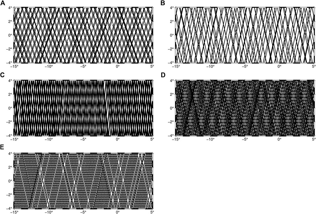
FIGURE 1. Ground tracks of (A) Jason-1/GM, (B) Envisat, (C) Cryosat-2, (D) SARAL/AltiKa, and (E) HY-2A/GM.
Reference Gravity Field
In implementing the remove-restore procedure, a global geopotential model (otherwise known as reference gravity field) is required. The reference gravity field of one quantity (which in this case is deflections of the vertical) is removed from its corresponding observed deflections of the vertical to obtain residual deflections of the vertical. The residual deflections of the vertical are then used to construct the residual gravity anomalies. Full gravity anomalies are later obtained by restoring the removed reference gravity field (now in the form of gravity anomalies). The removal of the reference gravity field ensures a more statistically homogeneous and smoother model. Also, it has the effect of ensuring that the gravity field outside the data extent is accounted for (Andersen, 2013). EGM2008 is expressed as coefficients of spherical harmonics and has a maximum degree of 2,190 (Pavlis et al., 2012). It was obtained from the International Centre for Global Earth Models (http://icgem.gfz-potsdam.de/).
Dynamic Topography
In the computation of gravity anomalies, the SSH data must initially be reduced to geoid heights. To achieve this, the time-dependent topography of the surface of the sea must be removed. It is well known that the geoid is linearly related to the mean sea surface through the mean dynamic topography (MDT) of the ocean surface. Therefore, to compute the geoid heights, this research used the mean dynamic topography DTU15MDT, obtained from the Technical University of Denmark. It is a product derived from EIGEN-6C4 and DTU15MSS mean sea surface model (Knudsen et al., 2016). The time-independent sea surface topography was removed through filtering similar to the method of Hwang et al. (2002).
Computation of Gravity Anomalies
The
Geoid gradients,
where
where
With reference to the remove-restore technique described in Figure 2, the computed components of deflections of the vertical are reduced to their residual version by subtracting EGM2008-simulated deflection components from them. The reference vertical deflections were simulated at the maximum degree/order of 2,190.
where
where
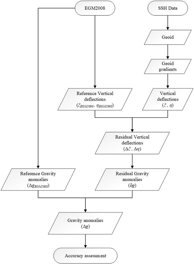
FIGURE 2. Remove-restore technique used.
Reviewed literatures have shown that for most altimetry-derived deflections of the vertical, the north component is often times more accurate than the east component. This is attributable to the inclinations of the satellites which usually are towards the north. The effect of this accuracy imbalance propagates to the resultant gravity anomalies derived from the deflections of the vertical (Small and Sandwell, 1992; Zhang, 2017; Wan et al., 2020b). In order to nullify this effect on the derived gravity anomaly model, weights are assigned to the vertical deflection components based on the covariance between them, and their error variances relative to the reference gravity field model. The residual gravity anomaly is derived from each component,
Using the constraints described in Eq. 9, the weights,
where
Results
The computed vertical deflection components are shown as Figure 3. They were validated by comparing them with simulated components from EGM2008 at maximum degree/order 2,190. The result of this comparison is summarized in Table 2. With regard to standard deviation of differences, it can be seen from Table 2 that the accuracy of the north component is slightly better than the east component by almost three times. A visual inspection shows that, in general, the positive deflections of the north component (Figure 3A) have a SW/NE orientation, whereas there is no distinct orientation in the east component (Figure 3B).
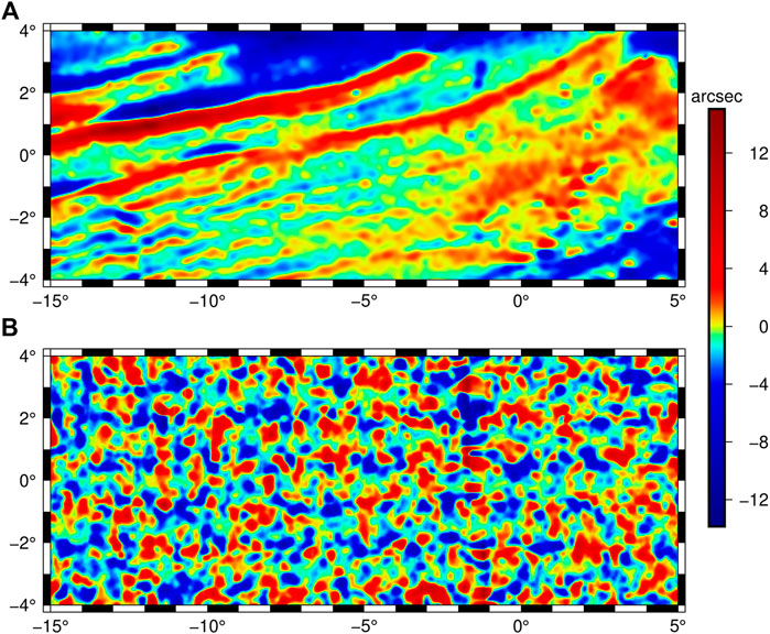
FIGURE 3. Computed vertical deflections: (A) North component, (B) East component.
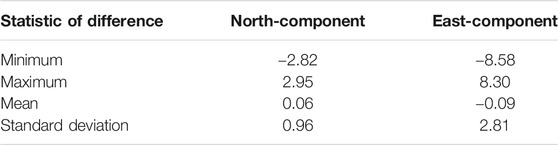
TABLE 2. Summary statistics of vertical deflection components compared with EGM2008-simulated components (unit: arcsecond).
With reference to Eqs. 8–10, Table 3 is a compilation of the vertical deflection components’ error variances, covariance and their respective weights used for the construction of the residual gravity anomaly. The constructed gravity anomaly model is shown in Figure 4. It compares well with gravity anomalies from EGM2008, DTU13 (obtained from the Technical University of Denmark) and SIOv28 (obtained from Scripps Institution of Oceanography) used as reference models. A summary of this comparison is presented in Table 4. Figure 5 shows similar histograms of gravity anomalies for the inverted model and the reference models; this is an attestation of high accuracy of the derived gravity anomalies. Figure 6 is a visual analysis of differences between the inverted gravity anomaly model and the reference models; this is a further attestation of the results presented in Table 4. On average, the model deviates from the reference models by −0.33 mGal. Further analysis of the histogram indicated that more than approximately 50% of gravity anomalies in the study region falls within the range of −80–80 mGal.
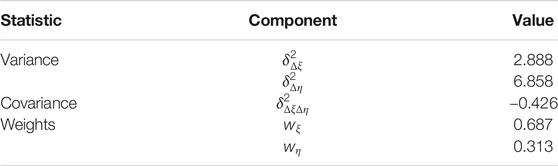
TABLE 3. Variances, covariance and weights of vertical deflection components.
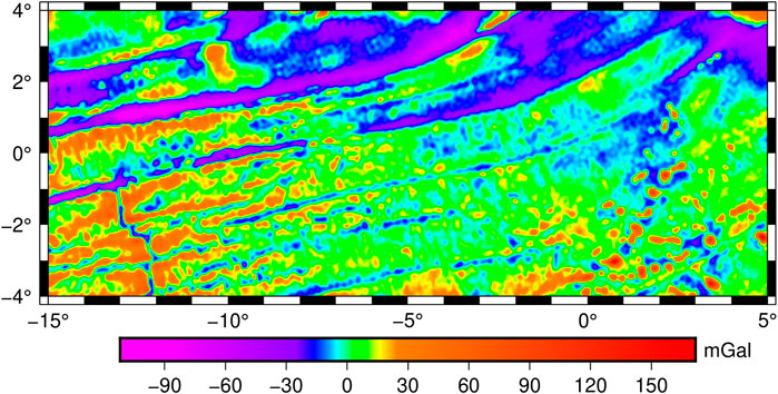
FIGURE 4. Inverted gravity anomaly model.
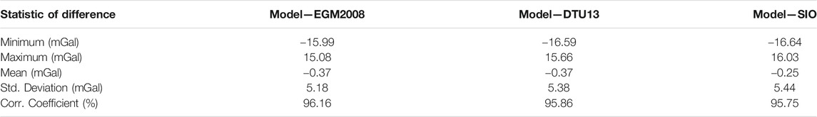
TABLE 4. Comparing modelled gravity anomaly with reference models.
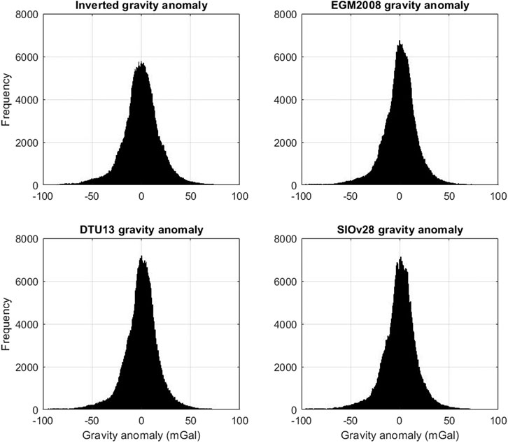
FIGURE 5. Comparing histograms of gravity anomaly models over the study region.
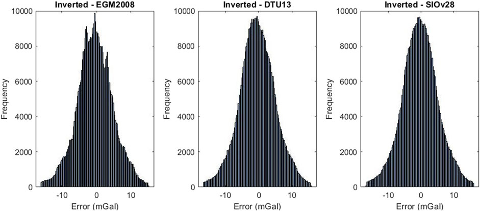
FIGURE 6. Histograms of gravity anomaly deviations from reference models.
Discussion
Comparing Derived Gravity Anomaly Model With Shipborne Gravimetry
The accuracy of the constructed gravity anomaly model is further analyzed by comparing it with gravity anomalies observed along tracks of ship cruises obtained from National Centers for Environmental Information of the National Oceanic and Atmospheric Administration (https://maps.ngdc.noaa.gov/viewers/geophysics/). However, the shipborne gravity data has the disadvantage of being very heterogenous with some erroneous observations made at some points. Some sources of these errors are: the absence of a uniform reference field at the time of measurement, drifting of the gravimeters, absence of base stations for references, etc. (Wessel and Watts, 1988). Therefore, in degree to amalgamate the shipborne gravity anomalies to a common reference, gravity anomalies simulated from EGM2008 were used as reference. With the exception of track RC1312, a second-degree polynomial model is then used to adjust the shipborne gravity anomalies. Track RC1312 was well adjusted by a first-degree polynomial. The adjustment model, given as Eq. 11, is applied separately on each ship track of observations.
where
The adjusted shipborne gravity anomalies are presented in Figure 7. From Figure 7, it can be seen that the northern half of the study region generally has lower gravity anomalies. Higher values can be observed at the southern part, especially in the south-west. The middle section has anomalies ranging approximately from −60 to 45 mGal. These observations generally agree with observations made from the constructed gravity model presented in Figure 4.
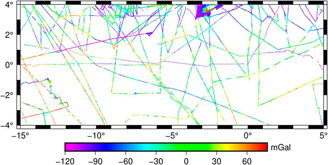
FIGURE 7. Shipborne gravity anomalies over the study region.
For each ship track, statistical summary analysis of the differences between the shipborne anomalies and modelled anomalies is computed; the results are given in Table 5. A total of 288 points were discarded due to their difference exceeding three times the standard deviation. Tracks that have relatively high standard deviations are: 88000811, CD5591, and V2604, with standard deviations of 8.50, 8.52, and 9.22 mGal, respectively. With regard to the error standard deviations, the most precise track is RC2602, it compared with the modelled gravity anomalies and yielded a standard deviation of 2.15 mGal. Without considering the mean errors, which denote the systematic errors, for major tracks of shipborne gravimetry, the standard deviations of the differences between the shipborne observations and the modelled gravity anomalies are smaller than 5.5 mGal. The ratios of the tracks with standard deviations smaller than 5.5 mGal and 6.0 mGal are about 71.4 and 78.6%, respectively. This index is close to the results of Table 4. Furthermore, from Table 5, it must be appreciated that the adjustment was done using EGM2008 as true values; therefore, the standard deviations of differences between the adjusted shipborne and EGM2008 gravity anomalies are virtually negligible. However, the magnitudes of the mean differences range within 1–20 mGal, which indicates the contribution from altimetry observations.
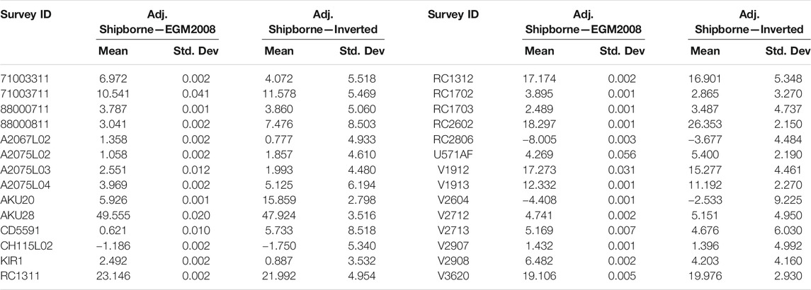
TABLE 5. Accuracy assessment of modelled gravity anomalies per track of shipborne gravimetry (unit: mGal).
In order to analyze the systematic errors depicted by the large mean errors in Table 5, the accuracy of gravity anomalies is assessed with respect to varying ocean depth. Table 6 is a summary of this analysis. The gravity anomalies are more accurate at depths deeper than 2,000 m. The mean deviation is approximately 5.09 mGal, which signifies the existence of some systematic errors. Therefore, in order to nullify the effects of these errors, observations whose deviation exceeded the mean deviation of the entire dataset were removed. This resulted in removal of values in shallow depths (depth range of 1,001–2,000 m), with the new results compiled in Table 7. It is obvious from Table 7 that the mean and standard deviation of differences escalate in shallow waters (i.e., in depth range of 1,001 ∼ 2,000 m). This shows that observations in shallow waters (depths > 2,000 m) were the main source of systematic differences.
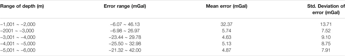
TABLE 6. Initial accuracy assessment of modelled gravity anomalies with respect to change in ocean depth.
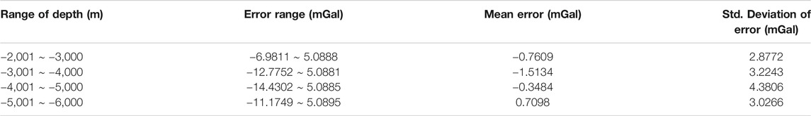
TABLE 7. Improved accuracy assessment of modelled gravity anomalies with respect to change in ocean depth.
Analyzing each satellite’s contribution in constructing the gravity anomaly model
In order to investigate the contribution of each satellite in the gravity field construction, the north,
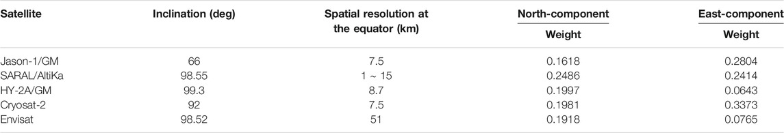
TABLE 8. Contribution of each satellite in establishing the deflections of the vertical.
It can be seen from Table 8 that SARAL/AltiKa contributed ∼25% in resolving the north component. This can be attributed to the range accuracy of its Ka-band signal. It is also possible that its good drifting phase spatial resolution (Verron et al., 2021) could be a factor, though this is sometimes lower than that of Cryosat-2. Approximately, 19% proportion of north component was realized from each of HY-2A/GM, Cryosat-2, and Envisat. This can be attributed to the geodetic spatial resolutions of these satellites, except for Cryosat-2 and Envisat which are not geodetic. Even though the datasets from Jason-1/GM are also geodetic, it contributed the lowest north component due to its lower spatial resolution. Jason-1/GM’s lower contribution in resolving the north component could also be attributed to its inclination of only 66°. On the other hand, due to this low inclination of 66°, Jason-1/GM contributed ∼28% of the east components, which is higher than that of SARAL/AltiKa. It was only surpassed by Cryosat-2 with ∼34%, which has one of the best spatial resolutions amongst altimetry satellite missions. For Cryosat-2, since it resolved more deflections in east component than north component, it seems that the effect of spatial resolution is larger than the inclination.
Conclusion
A regional gravity anomaly model of the Gulf of Guinea has been constructed through the remove-restore method. It was constructed from deflections of the vertical derived from five different altimetry missions. The north-component of vertical deflections was more accurate than the east-component by almost three times. Analysis of the vertical deflections (Table 8) revealed that, on average, SSH data from each satellite can contribute almost equally in resolving the north component. However, Cryosat-2, Jason-1/GM, and SARAL/AltiKa were the dominant contributors of the east component. The gravity anomaly model was constructed by assigning weights of 0.687 and 0.313 to the north and east components, respectively. A comparison of histograms (refer to Figure 5) of the computed gravity anomaly model with renowned models from EGM2008, SIOv28, and DTU13 showed similar results. The computed gravity anomaly averagely deviated from these reference models by −0.33 mGal. Further assessment was done by comparing it with quadratically adjusted shipborne free-air gravity anomalies. By excluding observations in shallow waters, the derived gravity field model compares well in depths deeper than 2,000 m.
Data Availability Statement
The original contributions presented in the study are included in the article/supplementary material, further inquiries can be directed to the corresponding author.
Author Contributions
Conceptualization, RA; methodology, both authors; data curation, both authors; funding acquisition, XW; formal analysis, RA; investigation, both authors; writing—original draft preparation, RA; writing—review and editing, both authors.
Funding
This research was funded by the National Natural Science Foundation of China (Nos. 42074017, 41674026); Fundamental Research Funds for the Central Universities (No. 2652018027); Open Research Fund of Qian Xuesen Laboratory of Space Technology, CAST (No. GZZKFJJ2020006); China Geological Survey (No. 20191006).
Conflict of Interest
The authors declare that the research was conducted in the absence of any commercial or financial relationships that could be construed as a potential conflict of interest.
Publisher’s Note
All claims expressed in this article are solely those of the authors and do not necessarily represent those of their affiliated organizations, or those of the publisher, the editors and the reviewers. Any product that may be evaluated in this article, or claim that may be made by its manufacturer, is not guaranteed or endorsed by the publisher.
Acknowledgments
The authors are grateful to ESA for providing GDRs of Envisat and Cryosat-2. We are appreciative to NASA/JPL and AVISO for providing GDRs of Jason-1/GM and SARAL/AltiKa, respectively. We thank the National Satellite Ocean Application Service of China for providing HY-2A/GM data. We are appreciative to DTU for providing DTU13, as well as SIO for providing SIOv28. We acknowledge the use GMT (Generic Mapping Tools) for drawing the maps. EGM2008 was provided by ICGEM/GFZ Potsdam. We recognize the use of shipborne gravity data which was provided by the National Centers for Environmental Information of the National Oceanic and Atmospheric Administration.
References
Ablain, M., Cazenave, A., Larnicol, G., Balmaseda, M., Cipollini, P., Faugère, Y., et al. (2015). Improved sea level record over the satellite altimetry era (1993-2010) from the Climate Change Initiative project. Ocean Sci. 11, 67–82. doi:10.5194/os-11-67-2015
Andersen, O. B., Knudsen, P., and Berry, P. A. M. (2010). The DNSC08GRA global marine gravity field from double retracked satellite altimetry. J. Geod. 84, 191–199. doi:10.1007/s00190-009-0355-9
Andersen, O. B., Knudsen, P., and Stenseng, L. (2016). “The DTU13 MSS (Mean Sea Surface) and MDT (Mean Dynamic Topography) from 20 Years of Satellite Altimetry,” in IGFS 2014: Proceedings of the 3rd International Gravity Field Service (IGFS), Shanghai, China, June 30 - July 6, 2014. Editors S. Jin, and R. Barzaghi (Cham: Springer), 111–121.
Andersen, O. B., and Knudsen, P. (2019). “The DTU17 Global Marine Gravity Field: First Validation Results,” in Fiducial Reference Measurements for Altimetry International Association of Geodesy Symposia.. Editors S. P. Mertikas, and R. Pail (Cham: Springer), 83–87. doi:10.1007/1345_2019_65
Andersen, O. B. (2013). “Marine Gravity and Geoid from Satellite Altimetry,” in Geoid Determination: Theory and Methods Lecture Notes in Earth System Sciences. Editors F. Sanso, and M. G. Sideris (Heidelberg: Springer-Verlag), 401–451. doi:10.1007/978-3-540-74700-0_9
Bazilian, M., Onyeji, I., Aqrawi, P.-K., Sovacool, B. K., Ofori, E., Kammen, D. M., et al. (2013). Oil, Energy Poverty and Resource Dependence in West Africa. J. Energ. Nat. Resour. L. 31, 33–53. doi:10.1080/02646811.2013.11435316
Becker, J. J., Sandwell, D. T., Smith, W. H. F., Braud, J., Binder, B., Depner, J., et al. (2009). Global Bathymetry and Elevation Data at 30 Arc Seconds Resolution: SRTM30_PLUS. Mar. Geodesy 32, 355–371. doi:10.1080/01490410903297766
Cazenave, A., Dieng, H.-B., Meyssignac, B., von Schuckmann, K., Decharme, B., and Berthier, E. (2014). The rate of sea-level rise. Nat. Clim. Change 4, 358–361. doi:10.1038/nclimate2159
Chander, S., and Majumdar, T. J. (2016). Comparison of SARAL and Jason-1/2 altimetry-derived geoids for geophysical exploration over the Indian offshore. Geocarto Int. 31, 158–175. doi:10.1080/10106049.2015.1041562
Dadzie, I., and Li, J. (2007). Determination of geoid over South China Sea and Philippine Sea from multi-satellite altimetry data. Geo-spatial Inf. Sci. 10, 27–32. doi:10.1007/s11806-006-0154-x
Hwang, C., and Chang, E. T. Y. (2014). Seafloor secrets revealed. Science 346, 32–33. doi:10.1126/science.1260459
Hwang, C., Hsu, H.-Y., and Jang, R.-J. (2002). Global mean sea surface and marine gravity anomaly from multi-satellite altimetry: applications of deflection-geoid and inverse Vening Meinesz formulaeflection-geoid and inverse Vening Meinesz formulae. J. Geodesy 76, 407–418. doi:10.1007/s00190-002-0265-6
Hwang, C. (1998). Inverse Vening Meinesz formula and deflection-geoid formula: applications to the predictions of gravity and geoid over the South China Sea. J. Geodesy 72, 304–312. doi:10.1007/s001900050169
Hwang, C., and Parsons, B. (1996). An optimal procedure for deriving marine gravity from multi-satellite altimetry. Geophys. J. Int. 125, 705–718. doi:10.1111/j.1365-246x.1996.tb06018.x
Hwang, C. (1999). A Bathymetric Model for the South China Sea from Satellite Altimetry and Depth Data. Marine Geodesy 22, 37–51. doi:10.1080/014904199273597
Knudsen, P., Andersen, O. B., and Maximenko, N. (2016). The updated geodetic mean dynamic topography model – DTU15MDT. Available at: http://lps16.esa.int/page_session122.php#998p.
Nguyen, V.-S., Pham, V.-T., Van Nguyen, L., Andersen, O. B., Forsberg, R., and Tien Bui, D. (2020). Marine gravity anomaly mapping for the Gulf of Tonkin area (Vietnam) using Cryosat-2 and Saral/AltiKa satellite altimetry data. Adv. Space Res. 66, 505–519. doi:10.1016/j.asr.2020.04.051
Olgiati, A., Balmino, G., Sarrailh, M., and Green, C. M. (1995). Gravity anomalies from satellite altimetry: comparison between computation via geoid heights and via deflections of the vertical. Bull. Géodésique 69, 252–260. doi:10.1007/BF00806737
Ophaug, V., Breili, K., and Andersen, O. B. (2021). A coastal mean sea surface with associated errors in Norway based on new-generation altimetry. Adv. Space Res. 68, 1103–1115. doi:10.1016/j.asr.2019.08.010
Osaretin, I. (2011). Energy Security in the Gulf of Guinea and the Challenges of the Great Powers. J. Soc. Sci. 27, 187–191. doi:10.1080/09718923.2011.11892919
Passaro, M., Nadzir, Z. A., and Quartly, G. D. (2018). Improving the precision of sea level data from satellite altimetry with high-frequency and regional sea state bias corrections. Remote Sensing Environ. 218, 245–254. doi:10.1016/j.rse.2018.09.007
Pavlis, N. K., Holmes, S. A., Kenyon, S. C., and Factor, J. K. (2012). The development and evaluation of the Earth Gravitational Model 2008 (EGM2008). J. Geophys. Res. 117, a–n. doi:10.1029/2011jb008916
Sandwell, D., Garcia, E., Soofi, K., Wessel, P., Chandler, M., and Smith, W. H. F. (2013). Toward 1-mGal accuracy in global marine gravity from CryoSat-2, Envisat, and Jason-1. The Leading Edge 32, 892–899. doi:10.1190/tle32080892.1
Sandwell, D. T., Müller, R. D., Smith, W. H. F., Garcia, E., and Francis, R. (2014). New global marine gravity model from CryoSat-2 and Jason-1 reveals buried tectonic structure. Science 346, 65–67. doi:10.1126/science.1258213
Small, C., and Sandwell, D. T. (1992). A comparison of satellite and shipboard gravity measurements in the Gulf of Mexico. Geophysics 57, 885–893. doi:10.1190/1.1443301
Soltanpour, A., Nahavandchi, H., and Ghazavi, K. (2007). Recovery of marine gravity anomalies from ERS1, ERS2 and ENVISAT satellite altimetry data for geoid computations over Norway. Stud. Geophys. Geod. 51, 369–389. doi:10.1007/s11200-007-0021-8
Verron, J., Bonnefond, P., Andersen, O., Ardhuin, F., Bergé-Nguyen, M., Bhowmick, S., et al. (2021). The SARAL/AltiKa mission: A step forward to the future of altimetry. Adv. Space Res. 68, 808–828. doi:10.1016/j.asr.2020.01.030
Villadsen, H., Andersen, O. B., Stenseng, L., Nielsen, K., and Knudsen, P. (2015). CryoSat-2 altimetry for river level monitoring - Evaluation in the Ganges-Brahmaputra River basin. Remote Sensing Environ. 168, 80–89. doi:10.1016/j.rse.2015.05.025
Wan, X., Annan, R. F., Jin, S., and Gong, X. (2020a). Vertical Deflections and Gravity Disturbances Derived from HY-2A Data. Remote Sensing 12, 2287. doi:10.3390/rs12142287
Wan, X., Annan, R. F., and Wang, W. (2020b). Assessment of HY-2A GM data by deriving the gravity field and bathymetry over the Gulf of Guinea. Earth Planets Space 72, 13. doi:10.1186/s40623-020-01291-2
Watson, C. S., White, N. J., Church, J. A., King, M. A., Burgette, R. J., and Legresy, B. (2015). Unabated global mean sea-level rise over the satellite altimeter era. Nat. Clim. Change 5, 565–568. doi:10.1038/nclimate2635
Wessel, P., and Watts, A. B. (1988). On the accuracy of marine gravity measurements. J. Geophys. Res. 93, 393–413. doi:10.1029/jb093ib01p00393
Zakharova, E. A., Krylenko, I. N., and Kouraev, A. V. (2019). Use of non-polar orbiting satellite radar altimeters of the Jason series for estimation of river input to the Arctic Ocean. J. Hydrol. 568, 322–333. doi:10.1016/j.jhydrol.2018.10.068
Zhang, S. (2017). Research on Determination of Marine Gravity Anomalies from Multi-Satellite Altimeter Data. Wuhan, China: Wuhan University.
Zhang, S., Sandwell, D. T., Jin, T., and Li, D. (2017). Inversion of marine gravity anomalies over southeastern China seas from multi-satellite altimeter vertical deflections. J. Appl. Geophys. 137, 128–137. doi:10.1016/j.jappgeo.2016.12.014
Zhu, C., Guo, J., Gao, J., Liu, X., Hwang, C., Yu, S., et al. (2020). Marine gravity determined from multi-satellite GM/ERM altimeter data over the South China Sea: SCSGA V1.0. J. Geod. 94, 50. doi:10.1007/s00190-020-01378-4
Keywords: sea surface heights, geoid gradients, vertical deflection, gravity anomaly, remove-restore technique, Gulf of Guinea
Citation: Annan RF and Wan X (2021) Recovering Marine Gravity Over the Gulf of Guinea From Multi-Satellite Sea Surface Heights. Front. Earth Sci. 9:700873. doi: 10.3389/feart.2021.700873
Received: 27 April 2021; Accepted: 14 July 2021;
Published: 23 July 2021.
Edited by:
D. Sarah Stamps, Virginia Tech, United StatesCopyright © 2021 Annan and Wan. This is an open-access article distributed under the terms of the Creative Commons Attribution License (CC BY). The use, distribution or reproduction in other forums is permitted, provided the original author(s) and the copyright owner(s) are credited and that the original publication in this journal is cited, in accordance with accepted academic practice. No use, distribution or reproduction is permitted which does not comply with these terms.
*Correspondence: Xiaoyun Wan, d2FueHlAY3VnYi5lZHUuY24=