 Joshua R. Chambers1*
 Mark W. Smith1
 Thomas Smith1Rudolf Sailer2
 Duncan J. Quincey1
 Jonathan L. Carrivick1
 Lindsey Nicholson3
 Jordan Mertes4
 Ivana Stiperski3
 Mike R. James5
- 1School of Geography and water@leeds, University of Leeds, Leeds, United Kingdom
- 2Department of Geography, Universität Innsbruck, Innsbruck, Austria
- 3Department of Atmospheric and Cryospheric Sciences, Universität Innsbruck, Innsbruck, Austria
- 4Centre for Environmental and Climate Science, Lund University, Lund, Sweden
- 5Lancaster Environment Centre, Lancaster University, Lancaster, United Kingdom
Spatially-distributed values of glacier aerodynamic roughness (z0) are vital for robust estimates of turbulent energy fluxes and ice and snow melt. Microtopographic data allow rapid estimates of z0 over discrete plot-scale areas, but are sensitive to data scale and resolution. Here, we use an extensive multi-scale dataset from Hintereisferner, Austria, to develop a correction factor to derive z0 values from coarse resolution (up to 30 m) topographic data that are more commonly available over larger areas. Resulting z0 estimates are within an order of magnitude of previously validated, plot-scale estimates and aerodynamic values. The method is developed and tested using plot-scale microtopography data generated by structure from motion photogrammetry combined with glacier-scale data acquired by a permanent in-situ terrestrial laser scanner. Finally, we demonstrate the application of the method to a regional-scale digital elevation model acquired by airborne laser scanning. Our workflow opens up the possibility of including spatio-temporal variations of z0 within glacier surface energy balance models without the need for extensive additional field data collection.
Introduction
The aerodynamic roughness length parameter (z0) is recognized as one of the key uncertainties in glacier surface energy balance (SEB) modeling (Cullen et al., 2007; Sicart et al., 2014; Litt et al., 2017; Fitzpatrick et al., 2019). It is defined as the topographically-controlled height above the surface at which horizontal wind velocity reaches zero (Stull, 1988; Garratt, 1992) and is typically derived from the direct observation of turbulent eddies through eddy covariance (Munro, 1989; Sicart et al., 2014; Fitzpatrick et al., 2019), or from extrapolation of log-linear fits of wind speed and air temperature profiles (Denby and Greuell, 2000; Brock et al., 2006; Quincey et al., 2017). Accurately quantifying z0 is essential for calculating and predicting glacier ablation because z0 is incorporated into calculations of the turbulent fluxes of sensible and latent heat between a surface and the adjacent atmosphere using the “bulk aerodynamic approach” (Hock, 2005). Using this approach, the sensible (H) and latent (LE) heat fluxes are defined as:
where
in which wind speed (
The turbulent fluxes commonly comprise ∼35–50% of a glacier SEB and have an increasingly important role in cloudy and windy conditions (Giesen et al., 2014), when they can become the dominant source of energy over short timescales (daily and sub-daily), contributing >75% of melt energy (Fausto et al., 2016). In maritime climates their dominance increases (Anderson et al., 2010). Despite the importance of z0, it is common for it to be generalized spatially across glacier surfaces and climatic zones, and through time (e.g., Lewis et al., 1998; Giesen et al., 2014; Bravo et al., 2017), at least partly because it is difficult to measure. Obtaining eddy covariance data or aerodynamic profiles from field measurements is challenging and provides only point-based z0 values; consequently, research has been driven toward estimation of spatially distributed z0 values from microtopography (Lettau, 1969; Munro, 1989), accelerated by the increasing availability of fine-resolution (sub-meter) and broad-scale topographic data.
Past work has identified that z0 is spatially and temporally dynamic, with topographic z0 values that have been validated against values from eddy covariance (EC) data or aerodynamic profiles (Brock et al., 2006; Irvine-Fynn et al., 2014; Miles et al., 2017; Quincey et al., 2017; Chambers et al., 2019; Fitzpatrick et al., 2019; Liu et al., 2020). In particular, the rapid data collection enabled by structure from motion photogrammetry (SfM; Smith et al., 2016b) and terrestrial laser scanning (TLS; Lemmens, 2011; Telling et al., 2017) has led to work focusing on development and validation of topographic methods, mostly concentrated on plot-scale data (tens of meters). However, the acknowledged scale and resolution-dependency of topographically-estimated z0 (Rees and Arnold, 2006) complicates the application of these methods to glacier-scale distributed energy balance models, because coarser resolution data lead to substantial underestimates of z0 and an order of magnitude change in z0 can double the calculated turbulent fluxes (Munro, 1989).
Initial efforts to produce glacier-scale maps of z0 have been promising (Smith et al., 2016a; Fitzpatrick et al., 2019; Smith et al., 2020), but here we seek to further these attempts by producing more robust topographic estimates of z0 at the glacier scale. We employ a simple workflow to correct for systematic underestimation of z0 values derived from coarser resolution data and show that the workflow can be used to produce first order estimates of z0 across the surrounding region. Specifically, we first present a multi-scale analysis of topographic z0 from data collected during the 2018 ablation season on Hintereisferner, Austria, and identify power law relations between data resolution and derived topographic z0. Second, through comparison with wind tower and EC data, we use these power laws to develop a correction factor for z0 estimates derived from coarse scale, widely available glacier surface topographic data, to bring them within one order of magnitude of likely true values, thus limiting the knock-on effects of over- or underestimation on the turbulent fluxes (c.f. Munro, 1989). Finally, we demonstrate the broader utility of the method by applying it to other nearby glacier surfaces covered by a freely available regional topographic dataset for Austria.
Data and Methods
Location
Field data were collected at Hintereisferner (46° 48′ N, 10° 47′ E) in the Austrian Alps (Figure 1), from 1 to 16 August 2018 during the Hintereisferner Experiment (HEFEX; Mott et al., 2020). Hintereisferner (HEF) is located high in the Rofenache catchment in the southern Otztal Alps, in the inner-alpine dry region (Strasser et al., 2018). The Rofenache catchment ranges from 1,891 to 3,772 m a.s.l, with an annual mean temperature of 2.5°C at 1,900 m a.s.l. (Strasser et al., 2018). Snow cover commonly persists from October through until June at elevations above 3,000 m a.s.l. Glaciers in the Otztal Alps, of which there are more than 50 (Abermann et al., 2009; Rastner et al., 2015), have been in retreat throughout the latter half of the 20th century and lost an average of 8.2% of their area between 1997 and 2006 (Abermann et al., 2009).
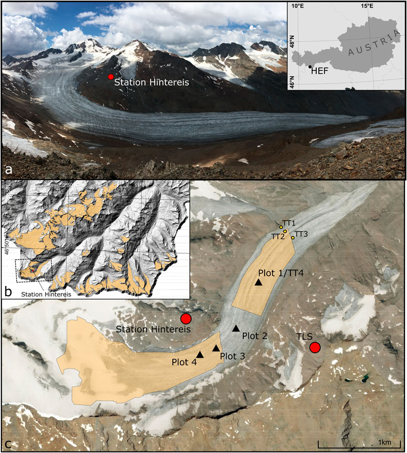
FIGURE 1. Location of Hintereisferner (HEF). (A) A digital photograph taken from the TLS installation with the location of HEF within Austria (inset). (B) The Ötztal Alps region, Tyrol, using part of the ALS DEM used in this study (Open Data Austria, 2020), highlighted with polygons of glaciers >0.5 km2 (Buckel et al., 2018). (C) Aerial imagery of HEF (ESRI; Orthophoto Tirol) with plot locations, upper/lower glacier TLS scan regions, Station Hintereis research base (2,964 m a.s.l.) and TLS (3,244 m a.s.l.).
HEF is ∼6 km long and ranges in elevation from ∼3,740 m to the current (2018) terminus at 2,498 m. Its present-day area is around 6.22 km2 but the glacier is receding rapidly, with an estimated reduction in area of 15% from 2001 to 2011, while the terminus retreated by around 390 m in the same decade (Klug et al., 2018). Mass balance records extend back to 1952/53 (Fischer, 2010) and HEF has been used as a type-site for gauging the overall health of Austrian glaciers and those of the wider European Alps, some of which, at current rates of retreat could be almost non-existent within a century (Vincent et al., 2017). Additional reconstructions suggest that HEF has been in near-constant retreat since the Little Ice Age, c.1855 (Greuell, 1992), with an increasing rate of mass loss as its tributary glaciers have become detached over the last two centuries (Fischer, 2010).
HEF has been the subject of a multitude of studies. Mass balance has been recorded using ablation stakes (Blümcke and Hess, 1899; Van De Wal et al., 1992; Kuhn et al., 1999) and numerical modelling (Escher-Vetter, 1985; Greuell, 1992; Schlosser, 1997; Fischer, 2010; Klug et al., 2018; Wijngaard et al., 2019). Remotely sensed data from airborne and satellite platforms have been used to study the glacier surface (Fritzmann et al., 2011), its reflectance properties (Koelemeijer et al., 1993) and allowed it to be included in valuable regional glacier inventories that document the decline of ice masses in the Alps (Patzelt, 1980; Lambrecht and Kuhn, 2007).
Data Collection
Data collection consisted of two main components: topographic surveys at multiple scales and meteorological data collection. Four plots were selected in the field (Figure 2), chosen to be as distinct in surface appearance as possible bearing in mind the safety risk associated with installing instrumentation and manually surveying very steep or heavily crevassed plots. Plot 1 (Figure 2A), the furthest down-glacier, was crosscut by supraglacial meltwater channels and was the most modified by melt processes having been exposed the longest after snowline retreat. Plot 2, shown in Figure 2B, appeared smoother than Plot 1, with some low (<0.2 m) flow-parallel ridges, some perpendicular crevasse traces and small moulins. Plot 3 was centered on an area of streamlined, well defined longitudinal ridges with no discernable cross-glacier features (Figure 2C). Plot 4 was the smoothest visually, with only minor surface variability and some small meltwater channels (Figure 2D).
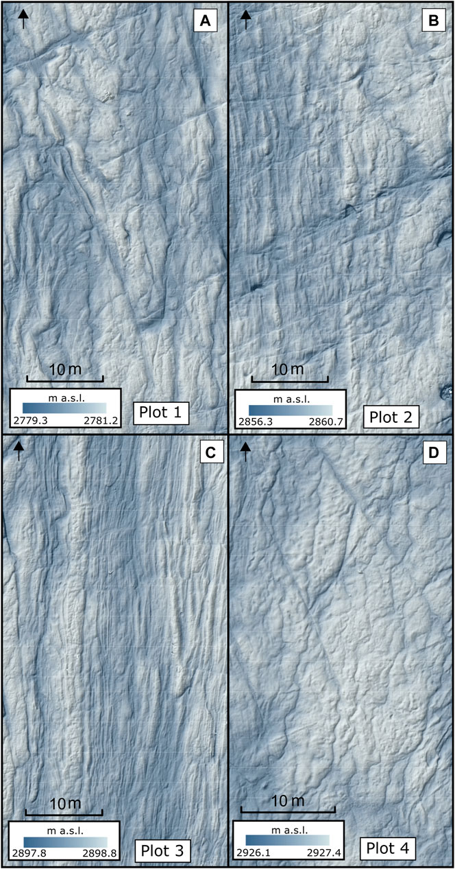
FIGURE 2. Examples of hillshaded DEMs generated from UAV imagery of each Plot. Black arrows indicate glacier flow direction.
A wind tower was installed at each plot [see Aerodynamic z0Estimation (z0WT,z0EC)] during the period when topographic surveys were carried out. As fieldwork was completed near the peak of the ablation season, air temperatures were positive for the study duration (Figure 3A) with diurnal extremes of 3–4°C at night and 10–18°C during the day. The maximum temperature was 19.8°C recorded on 5th August and the minimum was 1.3°C on 8th August. Mean wind speed for the data collection period was 2.5 m s−1, although occasionally fluctuated above 5 m s−1 (Figure 3B). The maximum recorded was 7.7 m s−1 on 14th August, while the minimum was below the stall speed of the cup anemometers (<1 m s−1) on multiple occasions. Wind direction was recorded relative to the down-glacier direction and was predominantly around 165°, indicating the presence of down-glacier flow characteristic of density driven katabatic winds (Figure 3C), which were also observed by Mott et al. (2020). Convective storms accounted for the majority of precipitation, with notable events in the afternoons of the 1st, 6th, 10th, and 13th August.
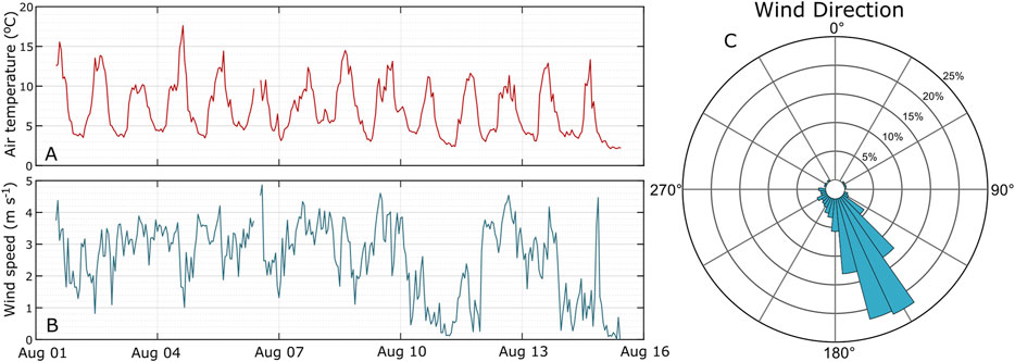
FIGURE 3. Meteorological data collected during study period. Both air temperature (A) and wind speed (B) are shown as hourly averages at ∼1 m above the glacier surface. A short gap in data on 6th August was caused by a hardware fault. Wind direction (C) is also hourly average with 0° set to the down glacier direction. All data are for Plot 1.
As part of HEFEX, four turbulence towers [TT1-4; see Aerodynamic z0Estimation (z0WT, z0EC)] were present throughout the data collection period (Mott et al., 2020). TT4 was located within Plot 1, while TT1-3 were installed further down-glacier. Independent estimates of z0 from these towers was used for validation of topographic and wind tower z0.
Topographic Surveys
Topographic z0 (z0DEM) was estimated using topographic data obtained via five methods covering a range of scales:
1. Small plots (10 m × 10 m): ground-based SfM using an Olympus OMD EM-10 camera mounted on a survey pole at ∼6 m above ground level on 10, 11, and 13 August. z0 from this method is referred to as z0Ground
2. Large plots (∼30 m × 70 m): ground-based SfM surveys encompassing [1], on 8, 10, 11, 12, and 13 August using the same camera as above but with the survey pole at ∼9 m above the surface (z0Pole)
3. Airborne plot surveys: SfM surveys of the same plots/dates as [2] using a DJI Phantom 3 uncrewed aerial vehicle (UAV) with gimbal-stabilized digital camera at ∼30 m above the surface (z0UAV)
4. Glacier-scale: the upper and lower glacier (see Figure 1) was surveyed on 3, 7, 12, and 16 August using a RIEGL VZ-6000 TLS situated on the true right of the valley, near the summit of “im Hinteren Eis”, a vantage point (Figure 1A) from which most of the glacier surface can be seen (z0TLS)
5. Regional-scale: Airborne Laser Scan (ALS) data, obtained from flights in 2001–2009 (between August and October) using ALTM3000 ALS, data freely available (Open Data Austria, 2020) (z0ALS).
Plot-Scale Structure From Motion Surveys (z0Ground, z0Pole, z0UAV)
SfM uses the principles of photogrammetry to digitally reconstruct surfaces or objects in 3D (Ullman, 1979; Brown and Lowe, 2005; Snavely et al., 2008) and has been used to obtain estimates of z0 on ice surfaces (Irvine-Fynn et al., 2014; Smith et al., 2016a; Chambers et al., 2019; Smith et al., 2020). We followed the same principles for each SfM survey, based on workflows and recommendations in James et al. (2017), O’Connor et al. (2017), completing surveys of Plot 1 on 10 and 13 August, Plot 2 on 8 August, Plot 3 on 11 August and Plot 4 on 12 August.
Camera specifications, camera calibration and survey area geometry (Table 1) were used to calculate the footprint of each image, which determined the distance between images required to achieve 60–80% overlap and the number of images needed for the survey area. Images were predominantly nadir and followed a regular grid pattern, with an additional ∼10% of images taken obliquely (<20° off nadir). All survey plots were marked out using a regular grid of 9 (z0Ground) or 21 (z0Pole and z0UAV) ground control points (GCPs), the locations of which were recorded using a Leica GS10 differential GPS, with a sub-centimeter mean accuracy for each plot. Typical 3D root mean square (RMS) control point error was ±0.03 m and RMS re-projection error was 1.66 pixels (2.6 µm). Uncertainty in z0 estimates associated with the SfM process is assumed to be negligible, following previous analysis in Chambers et al. (2019). Where z0DEM values are given for any plot, the standard deviation of the relevant plot is also given as a proxy for any further uncertainties, and the same is included for z0TLS values.
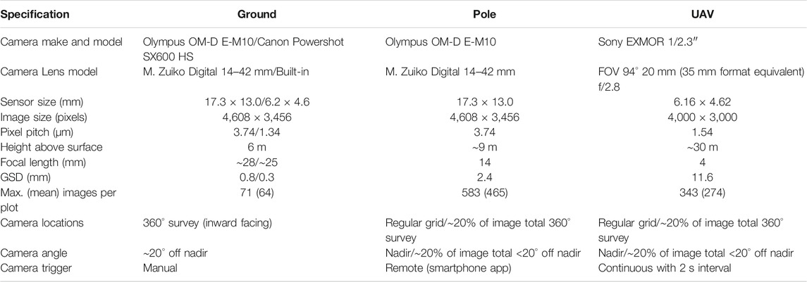
TABLE 1. Details of cameras used and survey design for SfM data collection.
Data were processed in Agisoft Photoscan Professional Edition Version 1.4.0 using the following settings: high accuracy, generic preselection enabled for all methods, reference preselection enabled for UAV surveys (as the position of the UAV is recorded for each image), camera calibration parameters F, Cx, Cy, K1-3, and P1 and P2 included, high reconstruction quality and aggressive depth filtering. Dense point clouds were imported into CloudCompare 2.10 (CloudCompare, 2020), where they were manually inspected/cleaned. Digital elevation models (DEMs) were constructed using linear interpolation with nearest non-empty neighbors, ensuring a regular grid shape with the top of the grid aligned with the direction of flow (roughly South-North). DEMs were produced at each of the grid resolutions shown in Table 2, using all of the neighborhood sizes also listed.
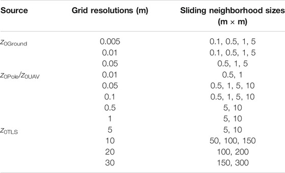
TABLE 2. List of grid resolutions and sliding neighborhood sizes used in multi-scale analysis.
Glacier and Regional-Scale Surveys (z0TLS, z0ALS)
A permanent in-situ Riegl VZ-6000 terrestrial laser scanner (TLS) was used to survey the majority of the glacier ablation zone using a near-infrared wavelength (1,050 nm) suited to snow and ice surfaces (University of Innsbruck, 2020a). The TLS is housed in a climate-controlled container near the summit of “im Hinteren Eis” (46.79586° N, 10.78277° E, 3,244 m a.s.l.). The point acquisition rate was approx. 23,000 points per second. Horizontal and vertical spatial resolution was ∼0.17 m at 1,000 m range, giving a theoretical density of 10 points per m2 mid-glacier, and 2 points per m2 at the head of the accumulation zone and near the terminus (University of Innsbruck, 2020b), due to the beam angle (Carrivick et al., 2015). Validation of scans from this TLS suggests <0.15 m difference to ALS data and <0.1 m between TLS scans (University of Innsbruck, 2020b). Surveys were split into two sections, upper and lower glacier, and carried out on 3rd, 7th, 12th, and 16th August 2018. TLS DEM creation was carried out using CloudCompare 2.10 (as described in Data Collection).
Regional (gridded) elevation data were acquired for the entire Austrian Alps at 10 m resolution (Open Data Austria, 2020). This regional product was created by interpolation of 2.5 m airborne laser scanning (ALS) data obtained during flights (details in Supplementary Table S1) over the Ötztal Alps, Tyrol, from 2006 to 2012 (Bollmann et al., 2011; Fritzmann et al., 2011; Sailer et al., 2012; Fischer et al., 2015). The reported vertical accuracy on relatively flat and smooth surfaces is ±0.07 m (σ = 0.07 m), with an absolute standard error on slopes <37° of ±0.04 m (Bollmann et al., 2011; Sailer et al., 2014). ALTM 3,100 and Gemini ALS sensors were used in the Tyrol area, with an average density of 0.25 points m−1. Glacier outlines were taken from the Austrian Glacier Inventory 4 (Buckel et al., 2018; Buckel and Otto, 2018).
Topographic z0 Estimation and Correction Factor Development
z0 was estimated from topographic datasets using the DEM-based method of Smith et al. (2016b) alongside a sliding neighborhood operation, wherein an operation is applied to each cell of a grid with a specified number of surrounding cells forming the neighborhood. The center of the neighborhood then slides to next cell until the operation has been applied to the entire grid. For this study, the sliding neighborhood function within MATLAB© R2017a was used. This approach is similar to that used by Fitzpatrick et al. (2019) but differs in how each parameter is defined. Most DEM methods, including those of Smith et al. (2016b), Fitzpatrick et al. (2019) and that used here, are based on the Lettau (1969) equation
where for each neighborhood, 0.5 is the average drag coefficient of roughness elements, h* is their average vertical extent [here we used twice the standard deviation of elevations over the detrended mean plane, mm, following Munro (1989)], s represents average silhouette area (mm2) and SA is the surface area of the neighborhood in the horizontal plane (mm2). s was calculated as the sum of the heights (mm) of all cells which visible above their respective preceding cell, as seen from the prevailing down-glacier wind direction, multiplied by cell width (mm). Detrending was performed on each neighborhood by removing the best-fit plane. TLS- and ALS-derived DEMs were additionally detrended by subtracting the moving mean calculated at 5 x grid resolution, which removed coarse scale topography but preserved finer scale topographic variability, i.e., perturbations of <1 m (Glenn et al., 2006; Smith, 2014). Resolution dependence was investigated by deriving z0DEM from grids with incrementally increased resolutions as listed in Table 2, while scale dependence was investigated by incrementally increasing neighborhood sizes.
Power law behavior displayed at Plot 1 (surveys from Day 10) was used to develop correction factors for each resolution. Correction factors were based on the quotient of modelled z0 for different grid resolutions and wind tower-derived z0 (z0WT), which was available from more locations across the glacier than z0 derived from turbulence towers (z0EC). Correction factors (CF) were calculated using:
where Res is a given resolution, a is the intercept and b is the corresponding gradient of a linear model fitted to a plot of log10 transformed grid resolution and z0DEM. The model fitted to the Plot 1 Day 10 data had a goodness of fit of r2 = 0.4, RMSE of 3 mm and p < 0.01, for 49 data points (47 degrees of freedom). The residuals of the model were normally distributed and displayed homoscedasticity when plot against predicted values. While some scatter remained in corrected z0DEM values, the predictive performance of the linear model was superior to non-linear models which were also tested, which under-predicted z0DEM at coarser grid resolutions and over-corrected it as a consequence.
Correction factors were calibrated using the data from Plot 1, then validated with Plots 2, 3, 4, and data from Plot 1 on Day 13, then TLS DEMs of Hintereisferner. Finally, they were used to project z0DEM values for the ALS DEMs of other local glaciers. An index of correction factor values for grids with resolutions of 0.005 m up to 30 m is included in Table 3.
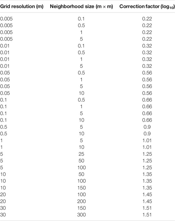
TABLE 3. Index of correction factors for each grid resolution.
Aerodynamic z0 Estimation (z0WT, z0EC)
Two wind towers provided point-based profile z0 measurements (z0WT). Since the prevailing wind was down-glacier the wind towers were placed toward the down-glacier end of each of the 30 m × 70 m plots, thereby capturing part of the tower footprint within the plots (Fitzpatrick et al., 2019). One tower was placed at Plot 1 for the duration of the study and the second “roving” tower, with the same set up as the first, was erected at Plot 2 from 5 to 8 August, Plot 3 from 8 to 12 August and Plot 4 from 12 to 15 August.
Each tower comprised five NRG 40 cup anemometers (uncertainty ±0.14 m s−1; starting at 0.3, 0.65, 1.22, 1.79, and 2.32 m above the surface, re-measured at each visit), one NRG 200P (uncertainty ±1.6°) wind vane and five shielded and passively-ventilated Extech RHT10 temperature and humidity loggers (uncertainty ±1°C and ±3%), following previous installations and processing steps (Quincey et al., 2017; Chambers et al., 2019). Data were averaged over 15 min intervals and processed using an r2 filter of 0.99 for log-linear profile fits, a minimum wind speed threshold of 1 m s−1 and a stationarity filter of 0.25°C m−1. A stability correction based on Monin-Obukhov (MO) similarity theory was applied to all profiles, as is common practice for glacier surfaces (Conway and Cullen, 2013; Stigter et al., 2017; Steiner et al., 2018).
Means and standard deviations for z0WT are given in Table 4. The limited duration of data collection and other sources of uncertainty affect the results given by the wind tower method, which can end up yielding very few data points due to the prevalence of katabatic winds; in these conditions, where the wind speed maximum is close to the surface, profiles do not adhere to MO theory (Denby, 1999). The longest duration of wind tower data collection was available for Plot 1 (15 days), which was used to calibrate the parameters of the correction factor (Eq. 6). Despite the small number of profiles that fit MO theory once corrected for atmospheric stability, the resulting dataset is more representative of typical atmospheric conditions than the shorter duration of other Plots. Values of z0WT from Plots 2, 3, and 4 were used for comparison with other z0DEM values, bearing in mind the inherent limitations of the method. Applying the MO stability correction ensured that, while the number of fitted profiles was smaller, profiles from katabatic conditions were not likely to be included erroneously.
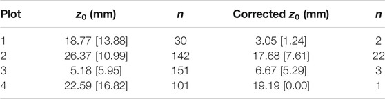
TABLE 4. Summary of z0WT (mm) from wind towers. Mean z0WT for the entire measurement duration for each plot is shown, including mean z0WT corrected for stability, with standard deviation (mm) in square brackets. n is the number of profiles that fit MO similarity theory.
The set-up of turbulence towers is described fully in Mott et al. (2020). On each tower, turbulence data were recorded by Campbell CSAT3 sonic anemometers at two levels, sampling at 20 Hz. Turbulent fluxes were calculated at 1 min intervals and averaged to 30 min, and z0EC (Table 5) was derived following Fitzpatrick et al. (2019), with assumed neutral stratification (z/L > 0 and z/L < 0.2) and additional quality control filters in place for atmospheric stability, wind direction (150–250°), minimum wind speed (2 m s−1), friction velocity (>0.1 m s−1) and stationarity. TT4 was located next to the wind tower in Plot 1, with mean z0EC for the entire study period providing an extra level of validation. Values of z0EC from TT1-3 were used to provide independent validation, but did not overlap with any Plots or the TLS data.
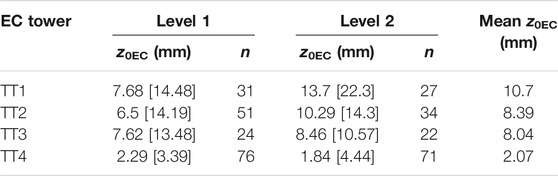
TABLE 5. Summary of z0EC (mm) from EC towers. Mean z0EC for the entire measurement duration for both levels at each tower is shown with standard deviation (mm) in square brackets, including overall mean. n is the number of values that fit the quality control criteria.
Results
Correction Factor Development
Scale and Resolution Relationships
Mean z0DEM as an average of all topographic methods, was 1.6 mm (σ = 3.3 mm), compared to 3.05 mm (σ = 1.24 mm) for z0WT and 2.07 mm (σ = 3.92 mm) for z0EC. Figure 4A shows that finer grid resolutions were associated with greater mean z0DEM values for each resolution between 0.005 m (mean z0DEM = 9.8 mm, σ = 7.5 mm) and 10 m (mean z0DEM = 0.1 mm, σ = 0.05 mm). At coarser grid resolutions, i.e., 10, 20, and 30 m, mean z0DEM increased by 0.1 –0.3 mm; these resolutions had fewer associated data points and the <0.5 mm variation is considered inconsequential. Larger z0DEM estimates were given at each resolution when larger neighborhood sizes were used, which increased the scale over which z0DEM was calculated. The average increase in z0DEM when neighborhood size was increased from the minimum was 0.7 mm (σ = 0.8 mm). Exceptions to this observation included resolutions of 0.005, 0.01, 5, and 20 m, where in each case there was one instance of decreased z0DEM with an increase of neighborhood size. Similar trends were observed for each of the other plots (Figures 4C–F).
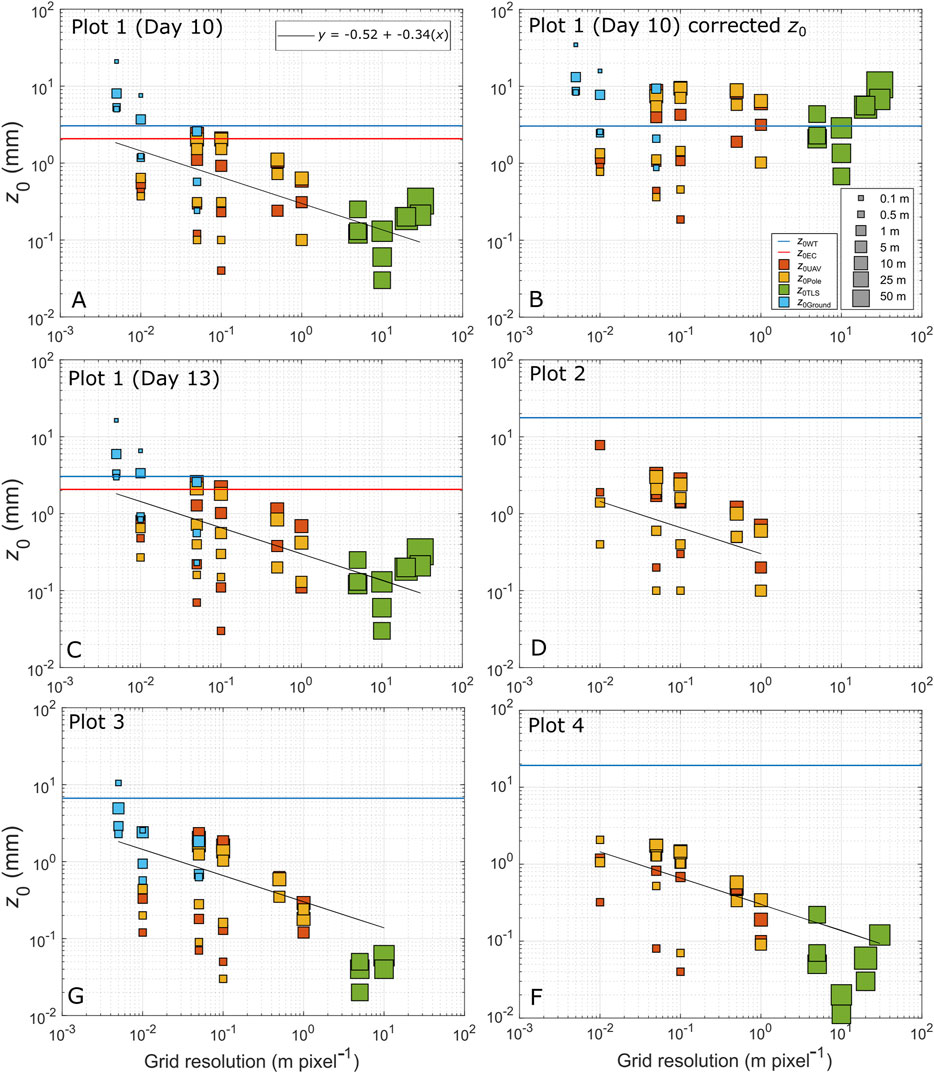
FIGURE 4. DEM grid resolution against z0DEM on log-log scale. Each data point represents z0DEM calculated using particular method, resolution and window size, extracted at the wind tower location within the Plot. (A) Plot 1 Day 10 uncorrected z0DEM, along with power law model developed using Plot 1 Day 10 data. (B) Corrected z0DEM for Plot 1 Day 10, where the correction factor for each DEM resolution is applied to raw input data. (C) Plot 1 Day 13 uncorrected z0DEM with Plot 1 Day 10 model to demonstrate its applicability elsewhere. (D) Plot 2 uncorrected z0DEM, again with model from Plot 1 Day 10 for illustration. (E) Plot 3 uncorrected z0DEM. (F) Plot 4 uncorrected z0DEM. The legends in (A) and (B) apply to all plots. The blue lines show z0WT for each plot (see Table 4) and red line show z0EC at Plot 1.
Correction Factor Calibration
Calibration of correction factors was performed on the data from Plot 1 Day 10 (Figure 4A). Once grid resolution and z0DEM were log10 transformed, the fitted linear model (with 95% confidence intervals) had an intercept of −0.52 ± 0.17 and slope of −0.34 ± 0.13 (RMSE = 3 mm; p < 0.01, 47 degrees of freedom). Correction factors increased with resolution from 0.22 at 0.005 m to 1.51 at 30 m. Application of the correction factors, as shown in Figure 4B, resulted in a shift in mean z0DEM from 1.6 to 3.04 mm (σ = 3.1 mm). On average, z0DEM was increased by 3.6 mm (σ = 3.1 mm). The mean difference between z0WT and corrected z0DEM was 2.2 mm (σ = 5.7 mm), and 3.15 mm (σ = 5.7 mm) between z0ECT and corrected z0DEM. Values of z0DEM at the finest resolutions were slightly over-corrected, but the performance of the correction factors at the coarsest resolutions is the main focus, since it is desirable that similar corrections can be applied to coarse resolution data in other locations.
Correction Factor Validation
The linear model from Plot 1 Day 10 was applied to the data from the remaining Plots (Figures 4C–F), where the fit and predictive capability was checked. The data from Plot 1 Day 13 (Figure 4C) showed only minor differences to Plot 1 Day 10, including some small increases in z0DEM, so the performance of the model was similar (r2 = 0.4). In Figure 4D, the data from Plot 2 (limited to UAV and Pole surveys) show a similar spread to those at Plot 1 and the mean corrected z0DEM was 3.8 mm (σ = 2.9 mm). The model appeared to describe the data less well (r2 = 0.1) due to relatively high scatter compared to the more extensive datasets at other Plots. At Plot 3 (Figure 4E) mean z0DEM was corrected to 1.7 mm (σ = 3.6 mm), which may have been an under-correction compared to the other Plots arising from a smaller sample of z0TLS data giving a weaker fit (r2 = 0.3). Plot 4 (Figure 4F) had the smallest z0TLS values (minimum 0.01 mm) and the highest z0WT values (19.2 mm). Here, mean z0DEM was corrected to 2.1 mm (σ = 2.6 mm), with the model fitting the data as well as in Plot 1 (r2 = 0.4).
Glacier-Scale Correction Factor Tests
Figure 5 shows corrected z0TLS calculated from glacier-scale TLS data, produced from 10 m resolution input data and 10 m × 10 m neighborhoods. The lower glacier scan exhibited a smaller range of z0TLS values (0.2–16.2 mm) than the upper (0.03–167.9 mm), with higher z0TLS attributed to an area covered by a thin layer of supraglacial debris. The mean lower glacier z0TLS was 1.7 mm (σ = 2.1 mm). The z0TLS values for the upper glacier covered four orders of magnitude, which reflected the presence of both heavy crevassing and icefalls alongside areas of smooth ice and those that were still snow-covered or recently exposed. The mean z0TLS for the upper glacier was 0.9 mm (σ = 4.3 mm), indicating that smoother surfaces were prevalent and that rougher surfaces caused extreme high z0TLS in a minority of cases. Inset panels (Figure 5i–v) show comparisons of the different z0DEM, z0WT and z0EC values for each Plot.
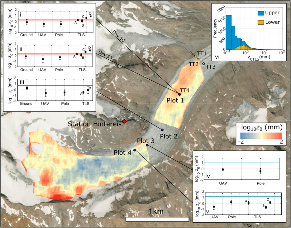
FIGURE 5. Upscaled and corrected z0TLS. Data shown is log10 transformed z0TLS at 10 m resolution obtained using 10 m × 10 m neighborhoods. Inset graphs (i–v) show comparisons of z0DEM from different sources. Ground, UAV and Pole data used 0.05 m resolution/0.5 m neighborhoods. TLS (A) used 5 m/50 m; TLS (B) 10 m/100 m; TLS (C) 20 m/200 m; TLS (D) 30 m/300 m. Error bars show the standard deviation of z0DEM at all tested grid resolutions for each method. Inset (vi) shows the distribution of z0TLS for the upper and lower glacier. The blue lines show z0WT for each plot (see Table 4) and red lines show z0EC at Plot 1.
Generally, corrected z0Ground, z0UAV and z0Pole was smaller than z0WT. Plot 1 Days 10 and 13 produced the most consistent z0DEM values across all methods (Figures 5i, ii), unsurprisingly given the model was calibrated to Plot 1. All z0DEM was lower than z0WT at Plots 2, 3, and 4; however, the observed z0WT values at Plots 2 and 4 were unexpectedly high (see Robustness of z0Estimates). Mean correction error for available data at Plots 1 and 3 was 1.9 mm (σ = 5.2 mm), 12 mm at Plot 2 and 16.1 mm at Plot 4. Plot 2 was not covered by TLS data so could not be compared fully. Plot 3 overlapped with the lower edge of the upper glacier scan, meaning z0TLS was not available at resolutions of 20 and 30 m.
Application to Regional Airborne Laser Scan Data
In order to demonstrate the potential for use of this upscaling approach at other locations without wind tower validation, z0DEM was calculated and corrected for glaciers surrounding Hintereisferner that are >0.5 km2 in area. Comparing corrected z0ALS and z0TLS values over Hintereisferner (Figures 6A,B), r2 for the upper and lower glacier was 0.6 and 0.5, respectively (both p < 0.01) suggesting that the distribution and values matched well (Supplementary Figure S1). Due to the temporal misalignment between the datasets, z0ALS was not expected to replicate z0TLS exactly, yet the spatial patterns and the distributions of both upper and lower glacier are similar, and are included here for demonstration in Figures 6A,B (insets). The sliding neighborhood operation allowed z0 to be estimated quickly for all glaciers at once from a single DEM of the region (Figure 7A). A correction factor of 1.35 was selected from the index (Table 3) according to resolution and neighborhood size (10 m resolution, 100 m × 100 m neighborhood size), and then applied to the uncorrected grid of log10z0ALS.
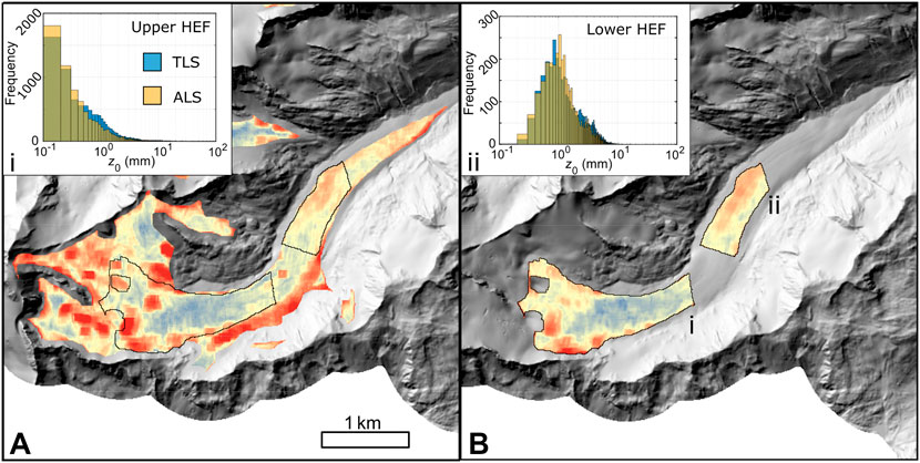
FIGURE 6. Corrected z0ALS for HEF (A) with TLS area overlain. Corrected z0TLS shown in (B). Comparison of distributions for upper (i) and lower (ii) glacier shown in insets–ALS data in front of TLS data.
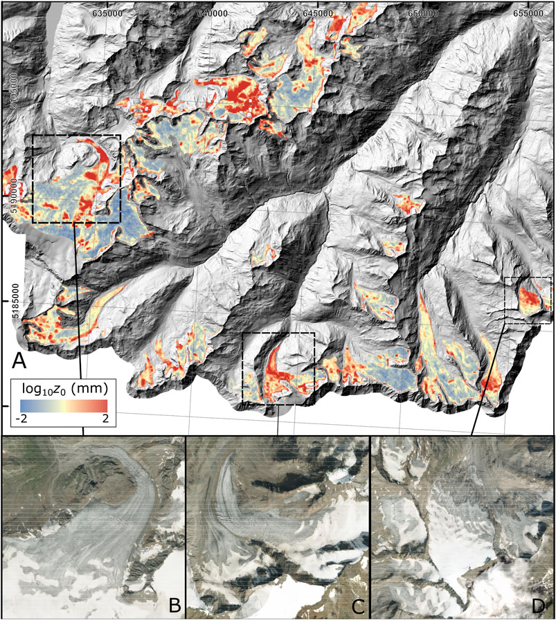
FIGURE 7. Corrected z0ALS for glaciers in the region around HEF (A). Lower images show enlarged imagery of select glaciers, including (B) Gepatsch Ferner, (C) Marzellferner and (D) Rotmoosferner (Source: ArcGIS World Imagery Basemap). Elevation data from Open Data Österreich (Digitales 10 m–Geländemodell aus Airborne Laserscan Daten). Glacier outlines from Austrian Glacier Inventory 4 (Buckel and Otto, 2018). Glaciers restricted to those with area >0.5 km2. z0ALS calculated using 100 m neighborhoods. All z0 is log10 transformed.
Regionally, corrected z0ALS was generally 0.1–10 mm (Figure 7A). Zones of z0 < 0.1 mm coincided with the highest elevation areas where persistent snow cover is likely, while zones of 10–100 mm covered areas of supraglacial debris, medial moraine (Figure 7C), light crevassing and rough ice. The roughest areas (>100 mm) matched heavily crevassed areas such as icefalls (Figure 7B), ice margins and where the glacier polygon overlapped with bedrock. Extreme values of z0ALS (>> 100 mm) were coincident with areas of very high relief, such as icefalls, heavy crevassing and ice-margins where uncertainty in elevation data is greatest. Visual comparison of z0ALS with inset images (Figures 7B–D) confirmed that expected spatial distributions of z0 can be derived from our workflow at the regional scale, as well as the glacier scale.
Discussion
Robustness of z0 Estimates
Several studies have demonstrated similarity between topographic and aerodynamic z0 over glaciers at the plot-scale (see Brock et al., 2006; Miles et al., 2017 for extensive compilations), lending confidence to our topographic estimates at finer resolutions. The values we obtained for 10 × 10 m and 30 m × 70 m plots using ground-based, UAV and pole-based surveys fall well within expected bounds (same order of magnitude) of z0 for an ablating Alpine glacier (∼0.1–10 mm; c.f. Munro, 1989; Brock et al., 2006), with the exception of the finest resolutions of 0.005 m. Power law behavior was observed in the distribution of 3D z0DEM against DEM grid resolution (Figure 4), as also shown by Rees and Arnold (2006) for 2D transect z0 estimates. Where Rees and Arnold (2006) noted a difficulty in obtaining a dataset that spanned a continuous range of scales and resolutions, modern survey techniques have afforded us the opportunity to collect and analyze data at resolutions across five orders of magnitude and at scales across four orders.
The z0DEM estimates within this study are also comparable to those given for different surfaces on Hintereisferner obtained using a slightly different topographic approach (Smith et al., 2020). A temporal model developed in Smith et al. (2020) noted that z0 was generally associated with the length of time that ice surface areas had been exposed by snow melt, as well as by physical factors such as surface gradient, which accounts for some of the highest z0 values. The z0TLS values for rougher surfaces like crevasses and a rock pedestal were more extreme in this study compared to the plots used by Smith et al. (2020), which were up to ∼20 mm, compared to 102 mm in this study. It is likely that our data incorporated some ice-marginal areas given the mismatch in resolutions between the TLS data and the glacier outline polygons derived from coarser resolution imagery. Other characteristic ice surfaces, such as the smooth/dirty ice, supraglacial channel and pressure ridge plots surveyed at the plot-scale in detail by Smith et al. (2020) compare well with the estimates of z0DEM here (within <5 mm generally).
The sliding neighborhood algorithm used to obtain z0DEM estimates in this study is similar to that described and used by Fitzpatrick et al. (2019), who used sliding neighborhoods to calculate a “drag parameter” (FD_local). Fitzpatrick et al. then attempted to account for fetch when calculating z0 for a point (z0_bloc) by equally weighting all cells within an area then finding their sum. Despite some minor differences in the initial calculation of each parameter, the range of values found for FD_local by Fitzpatrick et al. (2019) is the same as the range of corrected z0DEM values found in this study (∼10–5–∼100 m). For further comparison, we also calculated z0_bloc for the z0UAV grids of each Plot, by equally weighting z0 within all cells and finding their sum. We found that the given z0_bloc values from our Plots were at least an order of magnitude smaller than corrected z0UAV values. It is worth noting that the area used for calculating z0_bloc here was only ∼70 m × 30 m, compared to the ∼2,000 m × 2,000 m used by Fitzpatrick et al. (2019), so the smaller order of magnitude is likely to be a function of the smaller number of values within a plot. Additionally, we consider the sliding neighborhood method used here to be more practical when trying to model glacier-wide z0 for use in a distributed SEB model because it does not require topographic data from beyond the margins of the glacier; although fetch is not explicitly accounted for, doing so would require the incorporation of turbulence characteristics across different surfaces and especially near the margins of the glacier (Nicholson and Stiperski, 2020), which would detract from the intended simplicity of our approach.
A key area of uncertainty exists in the z0WT values derived from Plots 2 (17.86 mm) and 4 (19.18 mm), which were both greater than expected considering field observations of the surface characteristics, z0WT and z0EC values at other plots and those from similar glaciers (e.g., Brock et al., 2006). Confidence in the value at Plot 4 is low because only one z0 value was obtained after stability correction; conversely, confidence is higher for Plot 2, where the 22 values given (Table 4) suggest either i) potential underestimation by topographic methods or ii) a stronger wind speed gradient likely due to a near-surface wind speed maximum under katabatic conditions (c.f. Mott et al., 2020).While z0WT values were included for comparison, we acknowledge that the short duration of data collection at Plots 2, 3, and 4 (<4 days for each) reduces confidence in their results. It is typical to collect much longer time-series in order to ensure that the average aerodynamic properties of the surface are captured even after aggressive data filtering (Stull, 1988; Radić et al., 2017; Fitzpatrick et al., 2019). These uncertainties further highlight the merits of a topographic approach, which does not rely on a lengthy field campaign.
We are confident that the longer data collection period at Plot 1 (2 weeks) was sufficient for it to be used to calibrate the parameters of the correction factor and that, at worst, it indicated the likely order of magnitude of z0. This is supported by topographic estimates of z0, which were similar for Days 10 and 13, and by the mean z0EC values for the same Plot which was less than 1 mm smaller and had a standard deviation that would still put z0 within the same order of magnitude. Other theoretical and methodological flaws in the retrieval of z0 from wind profiles and EC data using MO similarity theory, such as the likely presence of katabatic winds (Mott et al., 2020) and collecting data over an ablating surface (Denby, 1999; Denby and Greuell, 2000; Litt et al., 2014; Radić et al., 2017), deterred us from seeking a perfect match between corrected z0DEM and z0WT.
Correction Factor Performance
The correction factor was developed by calibrating topographic z0 from Plot 1 with z0WT for the same plot, assuming z0DEM to be representative of a portion of the footprint of the wind tower (c.f. Fitzpatrick et al., 2019). Our goal was to match the wind-tower-derived z0 values to within an order of magnitude. Small differences in z0 will alter resultant turbulent flux values, but it is unreasonable to simply accept any one value as being absolute because z0 changes rapidly in both time and space over several orders of magnitude (Smith et al., 2016a; Smith et al., 2020). Furthermore, it is difficult to measure a “true” value of z0, as even EC data (often seen as the benchmark) relies to an extent on modeling and associated embedded assumptions (Cullen et al., 2007; Radić et al., 2017). Therefore, z0WT values were used as a calibration point to ensure z0DEM was calibrated to within an order of magnitude of the true z0. Of course, further aerodynamic data from this and other regions would strengthen the upscaling workflow developed here. However, this upscaling method provides a more reasonable estimate of distributed z0 than is achievable using aerodynamic methods by themselves or through the use of past topographic z0 techniques.
From visual inspection, and bearing in mind the absence of validation data beyond Hintereisferner itself, the correction factor appears to produce a realistic representation of spatial z0 variability at multiple scales (Figure 6) when resulting values are compared to past studies. Spatial patterns in the derived values are maintained and correspond to areas that appear smoother/rougher based on surface features identified in satellite imagery. Areas of dubiously high values (>102 mm) are coincident with areas where the DEM is least reliable, including heavily crevassed regions, icefalls and other areas of high relief (Sailer et al., 2014). While the distribution of z0 matches expectations from the perspective of surface roughness, it is worth noting that the footprint, or fetch, of each particular DEM cell is not considered. The fetch includes all aerodynamically important areas upwind of a point Kljun et al., 2015 which, over glaciers, has been observed to extend from ∼100 to 200 m, depending on the wind speed (Fitzpatrick et al., 2019). This leads to the question of how the sharp transitions between areas of contrasting roughness that can be seen in Figures 5, 6 can be accounted for in a straightforward model such as that used in this study, or indeed if they can be at all, as the nature of turbulent air flow over glaciers is extremely complex when considering the influence of the valley sides, different surfaces and tributary valleys (Stiperski and Rotach, 2016; Mott et al., 2020; Nicholson and Stiperski, 2020). It may be possible to account for fetch in topographic models in the future, considering advances in the availability of fine-resolution fields of meteorological variables such as wind speed (Sauter and Galos, 2016) and capabilities for modelling their interactions with terrain at small (100 m) scales (Fiddes and Gruber, 2014; Peleg et al., 2017). That being said, the topographic z0 methods employed here were developed only to use the properties of a surface to produce a value similar to an aerodynamically-derived value for the same point (Lettau, 1969; Munro, 1989); our workflow is intended to retain this rationale whilst indicating broader patterns. Additional complexities could be factored in with further work, depending on the application.
Implications
Use of the correction factor presented here allowed a realistic z0 value to be derived from a relatively coarse resolution DEM of Hintereisferner, Austria, of the type typically available for whole glacierized regions of the cryosphere. Additional testing and ground-truthing, ideally with sonic anemometers, would allow further calibration of the power laws and correction factors, especially in areas with varying debris sizes and coverage (e.g., Miles et al., 2017; Nicholson and Stiperski, 2020) and in areas covered by snow, that were not sampled in our study. Our workflow is an advance in the use of topographic methods for estimating z0 that can be applied (with caution until further validated) to other glaciers without the need for additional field data collection. It provides a more robust estimate of z0 than is achievable by collecting 2D transects, or by implementing z0 values borrowed from the literature and we foresee that the prevailing practice of using a constant or assumed z0 value in both distributed and single-point SEB models could potentially be eliminated.
A worthwhile additional step will be to develop the workflow for spatially distributed z0 grids established here into a model that includes a temporal dimension. Fully distributed z0 could then be incorporated in a distributed surface energy balance (SEB) model, to analyze the effects that this new quantification of z0 has on the turbulent fluxes and resultant meltwater production. This development would be especially useful when combined with the more widespread availability of national ALS campaign datasets (such as that used herein for Austria), or regional DEM datasets such as the ArcticDEM, the Reference Elevation Model for Antarctica and the High Mountain Asia DEM (Shean, 2017; Porter et al., 2018; Howat et al., 2019) and increasing availability of multi-temporal DEMs from platforms such as WorldView 2, Pléiades and Geo-Eye-1 (Belart et al., 2017; Shean, 2017). A work-flow diagram and example code for calculating corrected z0 is provided in the Supplementary Information (Supplementary Figure S2) to facilitate replication of the method, with the caution that full testing across different sites exhibiting a variety of surface characteristics, and using topographic data from a range of different sources, is still required.
Conclusion
We carried out a multi-scale investigation of topographic z0 over Hintereisferner, Austria. Data from SfM, TLS and ALS were employed to rapidly capture z0 at resolutions from sub-cm to 30 m. z0 values exhibited a power law behavior with data resolution. From this relationship we devised correction factors that adjusted topographic z0 so that it was within an order of magnitude of previously validated, more robust values from both finer resolutions and z0 calculated from wind profiles. While sensitivities and uncertainties in z0 estimates persist due to scale/resolution dependence and the simplification of aerodynamic processes, the method presented here has allowed z0 to be rapidly estimated at the glacier scale, capturing more detail and variability than is possible with point-scale or 2D techniques. We used the same upscaling method to demonstrate how topographic z0 can be estimated at the glacier scale across an entire region. Further analysis for sites within different climatic zones is required to calibrate the correction factors, but the workflow provides a robust foundation for obtaining spatially distributed z0 without the need for lengthy field campaigns with delicate meteorological equipment, by being compatible with regional elevation datasets that are increasingly becoming publicly available.
Data Availability Statement
The datasets supporting the conclusions of this article are available from the UK Polar Data Centre repository, DOI: https://doi.org/10.5285/57EB95F0-1650-4670-A1BB-8CCC90CB1C5F
Author Contributions
Fieldwork was carried out during the HEFEX campaign. JRC, TS and MS collected UAV, pole, ground and wind tower data. Turbulence tower data was collected by IS, LN and JM, and TLS data by RS. JRC performed data analysis and wrote the manuscript with supervision from MS and DQ. IS processed the turbulence data and provided manuscript feedback along with JLC, LN, JM, RS, and MJ.
Funding
Fieldwork was funded by an INTERACT Transnational Access grant awarded to MWS under the European Union H2020 Grant Agreement No. 730938. JRC is supported by a NERC PhD studentship (NE/L002574/1). IS was funded by Austrian Science Fund (FWF) grant T781-N32. Publication is covered by the University of Leeds UKRI block grant.
Conflict of Interest
The authors declare that the research was conducted in the absence of any commercial or financial relationships that could be construed as a potential conflict of interest.
Acknowledgments
We gratefully acknowledge the use of the TLS facility and data, financed by the University of Innsbruck and jointly operated by the Department of Geography and the Department of Atmospheric and Cryospheric Research. We thank the reviewers for their helpful and constructive feedback that greatly improved this manuscript. We also thank an reviewer for their comments on an earlier draft of the manuscript.
Supplementary Material
The Supplementary Material for this article can be found online at: https://www.frontiersin.org/articles/10.3389/feart.2021.691195/full#supplementary-material
References
Abermann, J., Lambrecht, A., Fischer, A., and Kuhn, M. (2009). The Cryosphere Quantifying Changes and Trends in Glacier Area and Volume in the Austrian Otztal Alps (1969-1997-2006). The Cryosphere 3, 205–215. doi:10.5194/tc-3-205-2009Available at: www.the-cryosphere.net/3/205/2009/
Anderson, B., Mackintosh, A., Stumm, D., George, L., Kerr, T., Winter-Billington, A., et al. (2010). Climate Sensitivity of a High-Precipitation Glacier in New Zealand. J. Glaciol. 56 (195), 114–128. doi:10.3189/002214310791190929
Blümcke, A., and Hess, H. (1899). Untersuchungen Am Hintereisferner. Verlag d. Dt. u. Österr. Alpenvereins
Belart, J. M. C., Berthier, E., Magnússon, E., Anderson, L. S., Pálsson, F., Thorsteinsson, T., et al. (2017). Winter Mass Balance of Drangajökull Ice Cap (NW Iceland) Derived From Satellite Sub-Meter Stereo Images. Cryosphere 11 (3), 1501–1517. doi:10.5194/tc-11-1501-2017
Bollmann, E., Sailer, R., Briese, C., Stötter, J., and Fritzmann, P. (2011). Potential of Airborne Laser Scanning for Geomorphologic Feature and Process Detection and Quantifications in High alpine Mountains. Zeit fur Geo Supp 55 (Suppl. 2), 83–104. doi:10.1127/0372-8854/2011/0055S2-0047
Bravo, C., Loriaux, T., Rivera, A., and Brock, B. W. (2017). Assessing Glacier Melt Contribution to Streamflow at Universidad Glacier, central Andes of Chile. Hydrol. Earth Syst. Sci. 21 (7), 3249–3266. doi:10.5194/hess-21-3249-2017
Brock, B. W., Willis, I. C., and Sharp, M. J. (2006). Measurement and Parameterization of Aerodynamic Roughness Length Variations at Haut Glacier d'Arolla, Switzerland. J. Glaciol. 52 (177), 281–297. doi:10.3189/172756506781828746
Brown, M., and Lowe, D. G. (2005). Unsupervised 3D Object Recognition and Reconstruction in Unordered Datasets. Proceedings of the Fifth International Conference on 3-D Digital Imaging and Modeling, Ottawa, Canada, 13-16 June 2005. doi:10.1109/3DIM.2005.81
Buckel, J., and Otto, J. C. (2018). ‘The Austrian Glacier Inventory GI 4 (2015) in ArcGis (Shapefile) Format’. Pangaea doi:10.1594/PANGAEA.887415
Buckel, J., Otto, J. C., Prasicek, G., and Keuschnig, M. (2018). Glacial Lakes in Austria - Distribution and Formation since the Little Ice Age. Glob. Planet. Change 164, 39–51. doi:10.1016/j.gloplacha.2018.03.003
Carrivick, J. L., Smith, M. W., and Carrivick, D. M. (2015). Terrestrial Laser Scanning to Deliver High-Resolution Topography of the Upper Tarfala valley, Arctic Sweden. Gff 137 (4), 383–396. doi:10.1080/11035897.2015.1037569
Chambers, J. R., Smith, M. W., Quincey, D. J., Carrivick, J. L., Ross, A. N., and James, M. R. (2020). Glacial Aerodynamic Roughness Estimates: Uncertainty, Sensitivity, and Precision in Field Measurements. J. Geophys. Res. Earth Surf. 125 (2). doi:10.1029/2019JF005167
CloudCompare (2020). CloudCompare. Available at: http://cloudcompare.org/(Accessed August 20, 2020)
Conway, J. P., and Cullen, N. J. (2013). Constraining Turbulent Heat Flux Parameterization over a Temperate Maritime Glacier in New Zealand. Ann. Glaciol. 54 (63), 41–51. doi:10.3189/2013AoG63A604
Cullen, N. J., Mölg, T., Kaser, G., Steffen, K., and Hardy, D. R. (2007). Energy-balance Model Validation on the Top of Kilimanjaro, Tanzania, Using Eddy Covariance Data. Ann. Glaciol. 46, 227–233. doi:10.3189/172756407782871224
Denby, B., and Greuell, W. (2000). The Use of Bulk and Profile Methods for Determining Surface Heat Fluxes in the Presence of Glacier Winds. J. Glaciol. 46 (154), 445–452. doi:10.3189/172756500781833124
Denby, B. (1999). Second-order Modelling of Turbulence in Katabatic Flows. Boundary-Layer Meteorol. 92 (1), 65–98. doi:10.1023/a:1001796906927
Escher-Vetter, H. (1985). ‘Energy Balance Calculations for the Ablation Period 1982 at Vernagtferner. Oetztal Alps’.A. Glaciol., 6, 158–160. doi:10.3189/1985AoG6-1-158-160
Fausto, R. S., As, D., Box, J. E., Colgan, W., Langen, P. L., and Mottram, R. H. (2016). The Implication of Nonradiative Energy Fluxes Dominating Greenland Ice Sheet Exceptional Ablation Area Surface Melt in 2012. Geophys. Res. Lett. 43 (6), 2649–2658. doi:10.1002/2016GL067720
Fiddes, J., and Gruber, S. (2014). TopoSCALE v.1.0: Downscaling Gridded Climate Data in Complex Terrain. Geosci. Model. Dev. 7 (1), 387–405. doi:10.5194/gmd-7-387-2014
Fischer, A., Seiser, B., Stocker Waldhuber, M., Mitterer, C., and Abermann, J. (2015). Tracing Glacier Changes in Austria from the Little Ice Age to the Present Using a Lidar-Based High-Resolution Glacier Inventory in Austria. The Cryosphere 9 (2), 753–766. doi:10.5194/tc-9-753-2015
Fischer, A. (2010). Glaciers and Climate Change: Interpretation of 50years of Direct Mass Balance of Hintereisferner. Glob. Planet. Change 71 (1–2), 13–26. doi:10.1016/j.gloplacha.2009.11.014
Fitzpatrick, N., Radić, V., and Menounos, B. (2019). ‘A Multi-Season Investigation of Glacier Surface Roughness Lengths through In Situ and Remote Observation’, The Cryosphere, 13, 1051–1071. doi:10.5194/tc-13-1051-2019
Fritzmann, P., Höfle, B., Vetter, M., Sailer, R., Stötter, J., and Bollmann, E. (2011). Surface Classification Based on Multi-Temporal Airborne LiDAR Intensity Data in High Mountain Environments A Case Study from Hintereisferner, Austria. Zeit fur Geo Supp 55 (Suppl. 2), 105–126. doi:10.1127/0372-8854/2011/0055S2-0048
Giesen, R. H., Andreassen, L. M., Oerlemans, J., and Van Den Broeke, M. R. (2014). Surface Energy Balance in the Ablation Zone of Langfjordjøkelen, an Arctic, Maritime Glacier in Northern Norway. J. Glaciol. 60 (219), 57–70. doi:10.3189/2014JoG13J063
Glenn, N. F., Streutker, D. R., Chadwick, D. J., Thackray, G. D., and Dorsch, S. J. (2006). Analysis of LiDAR-Derived Topographic Information for Characterizing and Differentiating Landslide Morphology and Activity. Geomorphol. 73 (1–2), 131–148. doi:10.1016/j.geomorph.2005.07.006
Greuell, W. (1992). Hintereisferner, Austria: Mass-Balance Reconstruction and Numerical Modelling of the Historical Length Variations’, J. Glaciol., 38(129), pp. 233–244. doi:10.3189/S0022143000003646
Hock, R. (2005). Glacier Melt: a Review of Processes and Their Modelling. Prog. Phys. Geogr. Earth Environ. 29 (3), 362–391. doi:10.1191/0309133305pp453ra
Howat, I. M., Porter, C., Smith, B. E., Noh, M.-J., and Morin, P. (2019). The Reference Elevation Model of antarctica. The Cryosphere 13 (2), 665–674. doi:10.5194/tc-13-665-2019
Irvine-Fynn, T. D. L., Sanz-Ablanedo, E., Rutter, N., Smith, M. W., and Chandler, J. H. (2014). Measuring Glacier Surface Roughness Using Plot-Scale, Close-Range Digital Photogrammetry. J. Glaciol. 60 (223), 957–969. doi:10.3189/2014JoG14J032
James, M. R., Robson, S., d'Oleire-Oltmanns, S., and Niethammer, U. (2017). Optimising UAV Topographic Surveys Processed with Structure-From-Motion: Ground Control Quality, Quantity and Bundle Adjustment. Geomorphology 280, 51–66. doi:10.1016/j.geomorph.2016.11.021
Kljun, N., Calanca, P., Rotach, M. W., Schmid, H. P., et al. (2015). A Simple Two-Dimensional Parameterisation for Flux Footprint Prediction (FFP). Geoscientific Model Development 8 (11), 3695–3713. doi:10.5194/gmd-8-3695-2015
Klug, C., Bollmann, E., Galos, S. P., Nicholson, L., Prinz, R., Rieg, L., et al. (2018). Geodetic Reanalysis of Annual Glaciological Mass Balances (2001-2011) of Hintereisferner, Austria. The Cryosphere 12 (3), 833–849. doi:10.5194/tc-12-833-2018
Koelemeijer, R., Oerlemans, J., and Tjemkes, S. (1993). Surface Reflectance of Hintereisferner, Austria, from Landsat 5 TM Imagery’, A. Glaciology., 17, 17–22. doi:10.3189/S0260305500012556
Kuhn, M., Dreiseitl, E., Hofinger, S., Markl, G., Span, N., and Kaser, G. (1999). Measurements and Models of the Mass Balance of Hintereisferner. Geografiska Annaler A 81 (4), 659–670. doi:10.1111/1468-0459.0009410.1111/j.0435-3676.1999.00094.x
Lambrecht, A., and Kuhn, M. (2007). Glacier Changes in the Austrian Alps during the Last Three Decades, Derived from the New Austrian Glacier Inventory’, Ann. Glaciol., 46, 177–184. doi:10.3189/172756407782871341
Lemmens, M. (2011). Terrestrial Laser Scanning. In: Geo-information. Geotechnologies and the Environment, vol 5. DordrechtSpringer, doi:10.1007/978-94-007-1667-4_6
Lettau, H. (1969). ‘Note on Aerodynamic Roughness-Parameter Estimation on the Basis of Roughness-Element Description’, J. Appl. Meteorol., 8(5), 828–832. doi:10.1175/1520-0450(1969)008<0828:noarpe>2.0.co;2
Lewis, K. J., Fountain, A. G., and Dana, G. L. (1998). Surface Energy Balance and Meltwater Production for a Dry Valley Glacier, Taylor Valley, Antarctica. A. Glaciology. 27, 603–609. doi:10.3189/1998AoG27-1-603-609
Litt, M., Sicart, J.-E., Helgason, W. D., and Wagnon, P. (2014). Turbulence Characteristics in the Atmospheric Surface Layer for Different Wind Regimes over the Tropical Zongo Glacier (Bolivia, $$16^\circ $$ 16 ∘ S). Boundary-layer Meteorol. 154 (3), 471–495. doi:10.1007/s10546-014-9975-6
Litt, M., Sicart, J.-E., Six, D., Wagnon, P., and Helgason, W. D. (2017). Surface-layer Turbulence, Energy Balance and Links to Atmospheric Circulations over a Mountain Glacier in the French Alps. The Cryosphere 11 (2), 971–987. doi:10.5194/tc-11-971-2017
Liu, J., Chen, R., and Han, C. (2020). Spatial and Temporal Variations in Glacier Aerodynamic Surface Roughness during the Melting Season, as Estimated at the August-One Ice Cap, Qilian Mountains, China. The Cryosphere 14 (3), 967–984. doi:10.5194/tc-14-967-2020
Miles, E. S., Steiner, J. F., and Brun, F. (2017). Highly Variable Aerodynamic Roughness Length (Z 0 ) for a Hummocky Debris-Covered Glacier. J. Geophys. Res. Atmos. 122 (16), 8447–8466. doi:10.1002/2017JD026510
Mott, R., Stiperski, I., and Nicholson, L. (2020). Spatio-temporal Flow Variations Driving Heat Exchange Processes at a Mountain Glacier. The Cryosphere 14 (12), 4699–4718. doi:10.5194/tc-14-4699-2020
Munro, D. S. (1989). Surface Roughness and Bulk Heat Transfer on a Glacier: Comparison with Eddy Correlation. J. Glaciol. 35 (121), 343–348. doi:10.3189/s0022143000009266
Nicholson, L., and Stiperski, I. (2020). ‘Comparison of Turbulent Structures and Energy Fluxes over Exposed and Debris-Covered Glacier Ice’, J. Glaciol., 66(258), 543. doi:10.1017/jog.2020.23
O’Connor, J., Smith, M. J., and James, M. R. (2017). Cameras and Settings for Aerial Surveys in the Geosciences: Optimising Image Data. Prog. Phys. Geogr. 41 (3), 325–344. doi:10.1177/0309133317703092
Open Data Austria (2020). Austria Digital Elevation Model. Available at: https://www.data.gv.at/katalog/dataset/land-ktn_digitales-gelandemodell-dgm-osterreich (Accessed August 20, 2020)
Patzelt, G. (1980). The Austrian Glacier Inventory: Status and First Results. Proceedings of the Riederalp Workshop. Riederalp, Switzerland, September 17-22, 1978.
Peleg, N., Fatichi, S., Paschalis, A., Molnar, P., and Burlando, P. (2017). An Advanced Stochastic Weather Generator for Simulating 2-D High-Resolution Climate Variables. J. Adv. Model. Earth Syst. 9 (3), 1595–1627. doi:10.1002/2016MS000854
Porter, C., Morin, P., Howat, I., Noh, M.-J., Bates, B., Peterman, K., et al. (2018). ArcticDEM. Harvard Dataverse, V1. doi:10.7910/DVN/OHHUKH
Quincey, D., Smith, M., Rounce, D., Ross, A., King, O., and Watson, C. (2017). Evaluating Morphological Estimates of the Aerodynamic Roughness of Debris Covered Glacier Ice. Earth Surf. Process. Landforms 42, 2541–2553. doi:10.1002/esp.4198
Radić, V., Menounos, B., Shea, J., Fitzpatrick, N., Tessema, M. A., and Déry, S. J. (2017). Evaluation of Different Methods to Model Near-Surface Turbulent Fluxes for an alpine Glacier in the Cariboo Mountains, BC, Canada. The Cryosphere, 11, 2897–2918. doi:10.5194/tc-11-2897-2017
Rastner, P., Nicholson, L., Sailer, R., Notarnicola, C., and Prinz, R. (2015). Mapping the Snow Line Altitude for Large Glacier Samples from Multitemporal Landsat Imagery. 8th International Workshop on the Analysis of Multitemporal Remote Sensing Images. Institute of Electrical and Electronics Engineers Inc. Annecy, France, 22-24 July 2015. doi:10.1109/Multi-Temp.2015.7245788
Rees, W. G., and Arnold, N. S. (2006). Scale-dependent Roughness of a Glacier Surface: Implications for Radar Backscatter and Aerodynamic Roughness Modelling. J. Glaciol. 52 (177), 214–222. doi:10.3189/172756506781828665
Sailer, R., Bollmann, E., Hoinkes, S., Rieg, L., Sproß, M., and Stötter, J. (2012). Quantification of Geomorphodynamics in Glaciated and Recently Deglaciated Terrain Based on Airborne Laser Scanning Data. Geografiska Annaler: Ser. A, Phys. Geogr. 94 (1), 17–32. doi:10.1111/j.1468-0459.2012.00456.x
Sailer, R., Rutzinger, M., Rieg, L., and Wichmann, V. (2014). Digital Elevation Models Derived from Airborne Laser Scanning point Clouds: Appropriate Spatial Resolutions for Multi-Temporal Characterization and Quantification of Geomorphological Processes. Earth Surf. Process. Landforms 39 (2), 272–284. doi:10.1002/esp.3490
Sauter, T., and Galos, S. P. (2016). Effects of Local Advection on the Spatial Sensible Heat Flux Variation on a Mountain Glacier. The Cryosphere 10 (6), 2887–2905. doi:10.5194/tc-10-2887-2016
Schlosser, E. (1997). Numerical Simulation of Fluctuations of Hintereisferner, Ötztal Alps, since AD 1850. A. Glaciol. 24, 199–202. doi:10.1017/s0260305500012179Available at: https://www.cambridge.org/core
Shean, D. (2017). High Mountain Asia 8-meter DEM Mosaics Derived from Optical Imagery, Version 1, NASA National Snow and Ice Data Center Distributed Active Archive Cent. Boulder, Colorado USA. doi:10.5067/KXOVQ9L172S2
Sicart, J. E., Litt, M., Helgason, W., Tahar, V. B., and Chaperon, T. (2014). A Study of the Atmospheric Surface Layer and Roughness Lengths on the High-Altitude Tropical Zongo Glacier, Bolivia. J. Geophys. Res. Atmos. 119 (7), 3793–3808. doi:10.1002/2013JD020615
Smith, M. W., Quincey, D. J., Dixon, T., Bingham, R. G., Carrivick, J. L., Irvine-Fynn, T. D. L., et al. (2016a). Aerodynamic Roughness of Glacial Ice Surfaces Derived from High-Resolution Topographic Data. J. Geophys. Res. Earth Surf. 121 (4), 748–766. doi:10.1002/2015JF003759
Smith, M. W., Carrivick, J. L., and Quincey, D. J. (2016b). Structure from Motion Photogrammetry in Physical Geography. Prog. Phys. Geogr. Earth Environ. 40 (2), 247–275. doi:10.1177/0309133315615805
Smith, T., Smith, M. W., Chambers, J. R., Sailer, R., Nicholson, L., Mertes, J., et al. (2020). A Scale-dependent Model to Represent Changing Aerodynamic Roughness of Ablating Glacier Ice Based on Repeat Topographic Surveys. J. Glaciol. 66, 950–964. doi:10.1017/jog.2020.56
Smith, M. W. (2014). Roughness in the Earth Sciences. Earth-Science Rev. 136, 202–225. doi:10.1016/j.earscirev.2014.05.016
Snavely, N., Seitz, S. M., and Szeliski, R. (2008). Modeling the World from Internet Photo Collections. Int. J. Comput. Vis. 80 (2), 189–210. doi:10.1007/s11263-007-0107-3
Steiner, J. F., Litt, M., Stigter, E. E., Shea, J., Bierkens, M. F. P., and Immerzeel, W. W. (2018). The Importance of Turbulent Fluxes in the Surface Energy Balance of a Debris-Covered Glacier in the Himalayas. Front. Earth Sci. 6 (October), 1–25. doi:10.3389/FEART.2018.00144
Stigter, E. E., Wanders, N., Saloranta, T. M., Shea, J. M., Bierkens, M. F. P., and Immerzeel, W. W. (2017). Assimilation of Snow Cover and Snow Depth into a Snow Model to Estimate Snow Water Equivalent and Snowmelt Runoff in a Himalayan Catchment. The Cryosphere 11 (4), 1647–1664. doi:10.5194/tc-11-1647-2017
Stiperski, I., and Rotach, M. W. (2016). On the Measurement of Turbulence over Complex Mountainous Terrain. Boundary-layer Meteorol. 159 (1), 97–121. doi:10.1007/s10546-015-0103-z
Strasser, U., Marke, T., Braun, L., Escher-Vetter, H., Juen, I., Kuhn, M., et al. (2018). The Rofental: a High Alpine Research basin (1890-3770 M a.s.l.) in the Ötztal Alps (Austria) with over 150 Years of Hydrometeorological and Glaciological Observations. Earth Syst. Sci. Data 10 (1), 151–171. doi:10.5194/essd-10-151-2018
Telling, J., Lyda, A., Hartzell, P., and Glennie, C. (2017). Review of Earth Science Research Using Terrestrial Laser Scanning. Earth-Science Rev. 169 (April), 35–68. doi:10.1016/j.earscirev.2017.04.007
Ullman, S. (1979). The Interpretation of Structure from Motion. Proceedings of the Royal Society of London. Series B, Biological Sciences, 203(1153), 405–426. doi:10.1098/rspb.1979.0006
University of Innsbruck (2020a). Permanent Terrestrial Laserscanner ‘Im Hinteren Eis’, Available at: https://www.uibk.ac.at/geographie/projects/i_he/ (Accessed August 20, 2020)
University of Innsbruck (2020b). Remotely Sensed Data. Available at: https://www.uibk.ac.at/projects/station-hintereis-opal-data/remotely-sensed-data/ (Accessed August 20, 2020)
Van De Wal, R. S. W., Oerlemans, J., and van der Hage, J. C. (1992). A Study of Ablation Variations on the Tongue of Hintereisferner, Austrian Alps’, J. Glaciol. 38(130), 319–324. doi:10.3189/S0022143000002203
Vincent, C., Fischer, A., Mayer, C., Bauder, A., Galos, S. P., Funk, M., et al. (2017). Common Climatic Signal from Glaciers in the European Alps over the Last 50 Years. Geophys. Res. Lett. 44 (3), 1376–1383. doi:10.1002/2016GL072094
Keywords: glacier, z0, structure from motion, terrestrial laser scanning, aerodynamic roughness
Citation: Chambers JR, Smith MW, Smith T, Sailer R, Quincey DJ, Carrivick JL, Nicholson L, Mertes J, Stiperski I and James MR (2021) Correcting for Systematic Underestimation of Topographic Glacier Aerodynamic Roughness Values From Hintereisferner, Austria. Front. Earth Sci. 9:691195. doi: 10.3389/feart.2021.691195
Received: 05 April 2021; Accepted: 14 May 2021;
Published: 28 May 2021.
Edited by:
Felix Ng, The University of Sheffield, United KingdomReviewed by:
Jakob Steiner, International Centre for Integrated Mountain Development, NepalRijan Bhakta Kayastha, Kathmandu University, Nepal
Copyright © 2021 Chambers, Smith, Smith, Sailer, Quincey, Carrivick, Nicholson, Mertes, Stiperski and James. This is an open-access article distributed under the terms of the Creative Commons Attribution License (CC BY). The use, distribution or reproduction in other forums is permitted, provided the original author(s) and the copyright owner(s) are credited and that the original publication in this journal is cited, in accordance with accepted academic practice. No use, distribution or reproduction is permitted which does not comply with these terms.
*Correspondence: Joshua R. Chambers, Z3lqcmNAbGVlZHMuYWMudWs=