Experimental Validation of N2 Emission Ratios in Altitude Profiles of Observed Sprites

Recent efforts to compare the sprite ratios with theoretical results have not been successfully resolved due to a lack of theoretical results for sprite streamers in varying altitudes. Advances in the predicted emission ratios of sprite streamers with a simple analytic equation have opened up the possibility for direct comparisons of theoretical results with sprite observations. The study analyzed the blue-to-red ratios measured by the ISUAL array photometer with the analytical expression for the sprite emission ratio derived from the modeling of downward sprite streamers. Our statistical studies compared sprite halos and carrot sprites where the sprite halos showed fair agreement with the predicted ratios from the sprite streamer simulation. But carrot sprites had lower emission ratios. Their estimated electric field has a lower bound of greater than 0.4 times the conventional breakdown electric field (E_k). It was consistent with the results of remote electromagnetic field measurements for short delayed or big/bright sprites. An unexpectedly lower ratio in carrot sprites occurred since sprite beads or glow in carrot sprites may exist and contribute additional red emission.

Introduction

A spectrophotometric diagnostic of sprites is of interest because the measured emission ratios indicate their characteristic energy and ionization degree in their discharge phenomena (Armstrong et al., 1998, 2000; Morrill et al., 2002). Previous spectral observations demonstrated two major visual emission bands: N₂ second positive band (2P, $C^3{\text{Π}}_u-B^3{\text{Π}}_g$ ) for blue emission, and N₂ first positive band (1P, $B^3{\text{Π}}_g$−$A^3{\text{Σ}}_u^{+}$ ) for red emission (Mende et al., 1995; Green et al., 1996; Hampton et al., 1996). One of the minor blue emission bands is the N₂⁺ first negative band (1N) for ionization associated emission (Armstrong et al., 1998, 2000; Morrill et al., 2002; Kanmae et al., 2010a, 2010b; Stenbaek-Nielsen et al., 2020). Observational techniques for sprite emission ratios have made significant progress using spectrophotometers (Armstrong et al., 1998; 2000), array photometers (Miyasato et al., 2002; 2003), optical spectra at 10,000 fps (Kanmae et al., 2010a, 2010b; Stenbaek-Nielsen et al., 2020) in ground campaigns, airplane campaigns (Morrill et al., 2002), and satellite measurements (Kuo et al., 2005; Mende et al., 2005; Adachi et al., 2006; Liu et al., 2006; Adachi et al., 2008; Kuo et al., 2008; Kuo et al., 2009). The investigation of the electrical discharge phenomena using remote sensing observation will help us study the impact of plasma chemistry and energy deposition by sprites in the middle atmosphere (Gordillo-Vázquez and Pérez-Invernón, 2021).

The sprite emission ratio of N₂ 2P to 1P can indicate the gained energy of accelerated electrons and the applied electric field in the streamer process and stands as a proxy for the electron energy leading to the emissions (Stenbaek-Nielsen et al., 2020). However, an inconsistent interpretation of sprite emission has appeared from past to now. Previous studies show sub-electric breakdown results (<1 E_k) in their observation (Morrill et al., 2002; Miyasato et al., 2003) where E_k is the electric field required for conventional breakdown. But their interpretation cannot reflect the high electric field (3−5 E_k) at a streamer head with a high emission rate. The estimated peak electric field in a streamer head provides insight into the sprite inception and the later development of sprite streamers from their initiation locations to lower altitude. The sprite emission estimation for a non-uniform streamer (Celestin and Pasko, 2010) complicates the electric field’s optical diagnostic method.

The analysis by Celestin and Pasko (2010) may explain why the electric field is estimated in the range of 1–2 E_k by Adachi et al. (2006). The emission ratios (2P/1N) reported by Kuo et al. (2005, 2009) indicated that the peak electric field of ∼3 E_k in sprites and ∼3.4–5.5 E_k in gigantic jets. These derived E-field values were underestimated for a peak electric field greater than 5 E_k in a sprite streamer simulation (Liu et al., 2006). Recently, Ihaddadene and Celestin (2017) developed analytic expressions from a streamer simulation to interpret the observed emission ratios at various altitudes. But they still lack spectroscopic data analysis to validate their sprite emission calculation at 50–90 km.

The interpretation of measured sprite emission at a sprite altitude of 50–90 km based on streamer modeling is still challenged (Celestin and Pasko, 2010). The neutral density varies exponentially with altitude. The transmittances for 2P and 1P emissions are sensitive to their observation path, as shown in Eq. 1. For sprite emission calculation in Eq. 2, their associated time coefficients depend on altitude. Besides, a sprite streamer’s characteristic spatial and temporal scale decreases exponentially with ambient neutral density at heights from 70 to 30 km. For example, the spatial scale of a sprite streamer varies from tens of meters at an altitude of 70 km to tens of centimeters at an altitude of 30 km (Pasko et al., 1998; Liu and Pasko, 2004). Figure 1 shows a streamer simulation at an altitude of 70 km. The non-uniform spatial distribution of their emission intensity at1P and 2P makes it impossible to easily estimate their sprite emission ratios, where the red and blue curves in Figure 1C indicate the 1P and 2P intensities along the streamer propagation direction. In Figure 2, the characteristic time coefficients in Eq. 2 vary with altitude. Even for a single streamer, the inhomogeneous emission intensity makes it difficult to estimate their emission ratios. We should consider the observation detection limits on their temporal and spatial scales and the synthesis effects of their spatial and temporal resolution on the emission measurement.

FIGURE 1

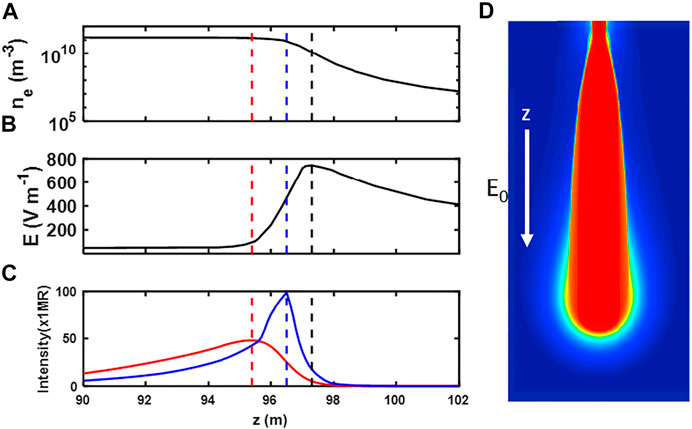
FIGURE 1. The inhomogeneous spatial distribution of electron density (n_e), electric field (E), and their 1P and 2P emission intensity in a sprite streamer. Here we show the computer simulation of a sprite streamer at time of 0.27 ms where the axial profiles of (A) electron density, (B) electric field and (C) N₂ 1P and 2P intensity are plotted along the propagating direction (z) with the ambient field 12 × $\frac{N}{N_0}$ kV cm⁻¹ (∼0.4 E_k), and at the altitude 70 km. The vertical red, blue and black dashed lines indicate the peaks of N₂ 1P, 2P emission and the electric field, respectively. A time lag between their peaks should be considered in sprite emission ratios. Panel (D) show the 2D cross section of the contour plot of positive streamer electron density of a streamer with positive streamer where electric field is downward (Ihaddadene and Celestin, 2017).

FIGURE 2

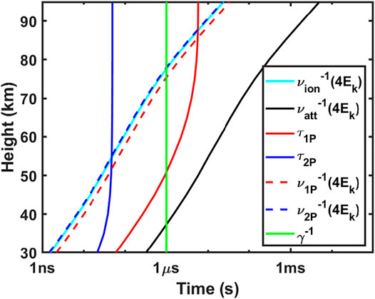
FIGURE 2. The characteristic time coefficient for calculating sprite emissions are compared in units of seconds at different altitudes. The characteristic time scales versus altitude where these time coefficients represent the ionization rate (cyan solid line) ν_ion⁻¹, the excitation rate ν_1P⁻¹ for N₂ $B^3{\text{Π}}_g$ state (red dashed line) at 4 E_k, the excitation rate ν_2P⁻¹ for $C^3{\text{Π}}_u$ state (blue dashed line) at 4 E_k, the lifetime τ_1P of N₂ 1P (red solid line), and the lifetime τ_2P of 2P band (blue solid line) emissions. The lifetimes of the N₂ 1P and 2P bands tend to be shorter due to the higher quenching rates (i.e., de-excitation processes) with increased neutral density at lower altitudes. The characteristic time for electron attachment rate ν_att⁻¹ at 4 E_k (black solid line) indicates the lifetime of streamer body where accumulated electrons at the streamer body are dissipated away after impact ionization by high electric field at the streamer head. The characteristic time (γ⁻¹ for the green line) for the growth rate γ in a sprite streamer is almost constant.

To approach this issue, we revisited similar analyses of the emission ratio by Adachi et al. (2006) based on analytic expressions from a streamer simulation (Ihaddadene and Celestin, 2017). Unlike ground and airplane campaigns, satellite measurement allow for a better transmittance, especially in the shorter wavelength range (e.g., the blue emission). The higher detected intensity in the blue emission may avoid underestimation of total blue emission when considering their transmittance. This study utilized the ISUAL dataset involving sprite blue and red emission onboard the FORMOSAT-2 satellite in The ISUAL array photometer. Analytical expressions for sprite emission ratios derived the analytical expressions for sprite emission ratios in an altitude profile of 50–90 km. After analyzing measured emission ratios, we validated an analytic expression for a streamer emission to interpret the observed emission ratios at various altitudes in Data Analyses. In the Summary, we summarized our results.

The ISUAL Array Photometer

The ISUAL payload on the FORMOSAT-2 satellite consists of an ICCD imager, a six-channel spectrophotometer (SP), and a dual-band array photometer (AP). The ISUAL AP contains blue (370–450 nm) and red (530–650 nm) bands of multiple-anode photometers at a sampling rate of 20 kHz. Each group of the AP has 16 vertically-stacked photomultiplier tubes (PMTs) with a combined field of view (FOV) of 22 deg (H) x 3.6 deg (V) (Chern et al., 2003; Mende et al., 2005; Frey et al., 2016). The ISUAL AP, imager, and SP are co-aligned at the centers of their respective FOVs.

FORMOSAT-2 is a Sun-synchronous satellite with 14 revisiting orbits per day. The ISUAL payload surveys transient luminous events (TLEs) and other luminescent emissions in the upper atmosphere globally with a side-looking view from an orbital altitude of 891 km. Wu et al. (2017) estimated a mean pointing error of 0.05° using star calibration with 1,296 stars from 2004 to 2014. The average pointing accuracy of ISUAL corresponds to a vertical resolution of 3.0 km at the maximum observation distance (3,500 km). Each AP channel has a half-height of 5.7–7.0 km for a distance of 2,900–3,500 km. Using satellite information recorded for TLE events, we can determine the altitude and location of the events based on the assumption that a bright center of a lightning-illuminated cloud has 10 ± 5 km (Kuo et al., 2008). Later, we constrained the uncertainty as a maximum value of the AP half height, considering the ISUAL pointing accuracy and the cloud height error after finally checking the top altitude of sprites at 90 km with an uncertainty of less than the AP half-height. The details of the uncertainty assessment on height are considered in Uncertainty in sprite emission ratios.

The AP band emission percentages B_k(h) for N₂ 1P and 2P band emission were used to convert the AP-measured brightness with blue and red filters into the specified total band emissions (2P and 1P, respectively). This was done while considering the atmospheric transmittance and instrument calibrations, including the filter wavelength range, lens transmittance, and detector response function (Frey et al., 2016). The percentage of the total band emission in an ISUAL AP is defined as the band percentage B_k(h), which is also a function of the altitude h and can be expressed as:

$B_k\left(h\right)=\frac{{\displaystyle \int {{\displaystyle I}}_k\left(h,\lambda \right)T\left(h,\lambda \right)R\left(\lambda \right)d\lambda }}{{\displaystyle \int {{\displaystyle I}}_k\left(h, \lambda \right)d\lambda }}(1)$

where $I_k(h,\lambda )$ is the intensity of emission lines in the specified band emission (N₂ 1P and 2P band emission) at an altitude h, which varies with the wavelength λ. $T(\lambda ,h)$ is the atmospheric transmittance, and $R\left(\lambda \right)$ is the AP response function (Frey et al., 2016).

We selected sprite events in the first 7 years (2005–2011) of satellite operation to avoid later-stage degradation in the AP sensitivities. Later, we used the band percentage B_k(h) to retrieve the AP-measured total emissions of the N₂ 2P and 1P bands. For $I_k\left(\lambda \right)$, we considered the N₂ 1P and 2P spectrum with a vibrational distribution function obtained by Gordillo-Vázquez et al. (2012), where the vibrational distribution is obtained from halos and sprites at 85 km and from sprites alone at 75 km. The significant changes are the unknown percentage of vibrational number v = 0 for the N₂ 1P spectrum. The uncertainty in the band percentage is typically ±15%. For the worst case, the error of the ratio is as high as 30%. We neglected the N₂⁺ 1N emission in the AP-measured blue emission. For an ambient electric field <2E_k, the contribution of N₂⁺ 1N emission to N₂ 2P is less than 2% according to similar calculations performed in Analytical Expressions for Sprite Emission Ratios.

Analytical Expressions for Sprite Emission Ratios

A measurement of the N₂ emission band ratio in sprites (e.g., 2P/1P or 1N/2P) is one of the most common remote optical diagnostic methods used to explore the physical conditions of complex sprite phenomena (Armstrong, 1998, 2000; Morrill et al., 2002; Miyasato et al., 2003; Kuo et al., 2005; Adachi et al., 2006; Adachi et al., 2008; Kuo et al., 2008; Kuo et al., 2009; Stenbaek-Nielsen et al., 2020). Sprite streamers associated with the first positive (1P), second positive (2P), and first negative (1N) band emission of N₂ can be analyzed using the analytical expressions for emission ratios in sprite streamer simulations (Celestin and Pasko, 2010; Pérez-Invernón et al., 2018). Here, we present the simplest expression for the sprite emission Ratio 1 $\left(r_{CB}\right)$ adopted in previous studies (Morrill et al., 2002; Miyasato et al., 2003; Kuo et al., 2005; Mende et al., 2005; Adachi et al., 2006; Adachi et al., 2008; Kuo et al., 2008; Kuo et al., 2009) in The Spatially Localized Instantaneous Emission Ratio. In The spatially and temporally integrated ratio, we modified the simplest expression by using an integral form for Ratio 2 $\left(R_{CB}\right)$ by considering the spatially and temporally integrated effects of the observations on the sprite emissions. Finally, we propose a complete presentation of Ratio 3 $\left(R_{CB}^{\ast }\right)$ considering the expansion of sprite streamers in The Spatially and Temporally Integrated Effect and the Experimental Growth of Streamer Expansion.

The Spatially Localized Instantaneous Emission Ratio

Following the calculation of streamer emissions (Pasko et al., 1997; Pasko et al., 1998; Barrington-Leigh and Inan, 1999; Liu et al., 2006; Celestin and Pasko, 2010; Ihaddadene and Celestin, 2017), the number density of the specified k-th excited state n_k is calculated using the population and depopulation equation:

$\frac{\partial n_k}{\partial \text{t}}=v_k{n}_e-n_k\left(A_k+q_{N_2}^k{n}_{N_2}+q_{O_2}^k{n}_{O_2}\right)+{\sum }_m{n}_m{A}_m(2)$

where ${\nu }_k$ is the excitation rate (s⁻¹), which depends on the applied electric field (Moss et al., 2006) with consideration of the cascade terms ${\displaystyle \sum _m{n}_m{A}_m}$, such as the cascading term $n_C$ for the N₂ 1P ($B^3{\text{Π}}_g$–$A^3{\text{Σ}}_u^{+}$) band emission. The number density of the specified k-th excited state spontaneously emits photons at a rate of the Einstein coefficient $A_k$, and ${\tau }_k$ is the lifetime defined by ${\tau }_k={\left(A_k+q_{N_2}^k{n}_{N_2}+q_{O_2}^k{n}_{O_2}\right)}^{-1}$. The quenching coefficients $q_{N_2}^k$ and $q_{O_2}^k$ are de-excitation rates by the ambient neutral density ($n_{N_2}$ or $n_{O_2}$ ). The lifetime ${\tau }_k$ of the k-th excited state is a function of height where larger neutral density at lower altitudes would decrease the lifetimes. If a maximum value of $n_k$ is reached $\left(\frac{\partial n_k}{\partial \text{t}}=0\right)$, the spatially localized instantaneous emission ratio $r_{k\prime k}$ is represented by (Celestin and Pasko, 2010),

$r_{k\prime k}=\frac{n_{k\prime }{A}_{k\prime }}{n_k{A}_k}=\frac{v_{k\prime }{A}_{k\prime }{\tau }_{k\prime }}{v_k{A}_k{\tau }_k},(3)$

where $k\prime$ -th and k-th excited states are emission bands of interest. In this study, the Ratio 1 is chosen as the ratio $r_{CB}$ of the N₂ 2P $\left(C^3{\text{Π}}_u-B^3{\text{Π}}_g\right)$ to N₂ 1P $\left(B^3{\text{Π}}_g-A^3{\text{Σ}}_u^{+}\right)$ band emission, which is given by:

$r_{CB}=\frac{n_C{A}_C}{n_B{A}_B}=\frac{v_C{n}_e{\tau }_C{A}_C}{\left(v_B{n}_e{\tau }_B+n_C{A}_C{\tau }_B\right)A_B}=\frac{v_C{A}_C{\tau }_C}{v_B{A}_B{\tau }_B}{\left(1+\frac{v_C{\tau }_C{A}_C}{v_B}\right)}^{-1}(4)$

where the cascading term ${\left(1+\frac{v_C{\tau }_C{A}_C}{v_B}\right)}^{-1}$ is considered as the cascading from the $C^3{\text{Π}}_u$ state into the $B^3{\text{Π}}_g$ state; ${\tau }_B$ and ${\tau }_C$ indicate the lifetime of their corresponding excited state $C^3{\text{Π}}_u$ and $B^3{\text{Π}}_g$, respectively. The number densities of the excited state $n_B=v_B{n}_e{\tau }_B+n_C{A}_C{\tau }_B$ and $n_C=v_C{n}_e{\tau }_C$ are obtained from Eq. 2 if a steady-state at its peak value is reached $\left(\frac{\partial n_k}{\partial \text{t}}=0\right)$. In Eq. 2, the number density $n_k$ of specified emission band is increased at the excitation rate $v_k$, which is proportional to the applied electric field. For a maximum electric field, the $n_k$ takes a time lag to reach its maximum value of specified band emission intensity.

Figure 1 illustrates a simulation result of the sprite streamer (Ihaddadene and Celestin, 2017). The panels (a), (b), and (c) of Figure 1 show the axial profiles of electron density, electric field and N₂ 1P/2P intensity along the propagating z-direction at a time of 0.27 ms and at an altitude of 70 km. For N₂ 1P/2P emission peaks (red/blue dashed line in Figure 1B), there exists a time lag between an emission peak and an electric field peak (black dashed line). Hence, Ratio 1 $\left(r_{CB}\right)$ in Eq. 4 is applied only for the ideal case. However, the optical diagnostic of sprites could not be spatially localized at a streamer head region and at an instantaneous time without considering time delays between their emission peaks. We should consider the temporally and spatially integrated effects compared with observation results. In the next section, we discuss further the temporally and spatially integrated impact on the Ratio 1 $r_{CB}$.

The Spatially and Temporally Integrated Ratio

Due to the AP detection limits both on spatial resolution (∼12 km at a distance 3,000 km) and temporal scale (50 µs), the spatially localized instantaneous emission ratio ${\mathit{r}}_{\mathit{CB}}$ should be considered as the time-integrated and spatial-integrated measurement by the AP. That means that Eq. 3 is spatially and temporally integrated. The spatially and temporally integrated ratio ${\mathit{R}}_{\mathit{k\text{'}k}}$ (noted by Ratio 2 hereafter) is:

$R_{k\prime k}={\displaystyle \iint r_{k\prime k}}\mathit{dtdV}=\frac{A_{k\prime }{\displaystyle \iint \left(\frac{\partial n_{k\prime }}{\partial \text{t}}\right)}\mathit{dtdV}}{A_k{\displaystyle \iint \left(\frac{\partial n_k}{\partial \text{t}}\right)}\mathit{dtdV}}(\mathrm{5a})$

$=\frac{A_{k\prime }{\tau }_{k\prime }{\displaystyle \iint v_{k\prime }{n}_e}\mathit{dtdV}}{A_k{\tau }_k{\displaystyle \iint v_k{n}_e}\mathit{dtdV}}=\frac{A_{k\prime }{\tau }_{k\prime }{v}_{k\prime }{N}_{e,k\prime }^{\ast }}{A_k{\tau }_k{v}_k{N}_{e,k}^{\ast }}(\mathrm{5b})$

where $N_{e,k}^{\ast }$ is the correction term for spatially and temporally integrating the electron density in the streamer region, and is expressed by ${\displaystyle \iint \left(\frac{\partial n_k}{\partial \text{t}}\right)}dtdV\equiv {\tau }_k{v}_k{N}_{e,k}^{\ast }$ where $N_{e,k}^{\ast }$ is defined by $v_k{N}_{e,k}^{\ast }\equiv {\displaystyle \iint v_k{n}_e}dtdV$ (Ihaddadene and Celestin, 2017) and in which the maximum contribution to the integration is at peak time of $n_k\left(t\right)$. Considering the cascading from the $C^3{\text{Π}}_u$ state into the $B^3{\text{Π}}_g$ state, we reformulated the Ratio 2 $\left(R_{CB}\right)$, which is expressed by

$R_{CB}=\frac{A_C{\tau }_C{v}_C}{A_B{\tau }_B{v}_B}\left(\frac{N_{e,C}^{\ast }}{N_{e,B}^{\ast }}\right){\left[1+\left(\frac{N_{e,C}^{\ast }}{N_{e,B}^{\ast }}\right)\frac{A_C{\tau }_C{v}_C}{v_B}\right]}^{-1}(6)$

where the cascading term is derived in a similar way in the Eq. 4 except for the addition of the term $\left(\frac{N_{e,C}^{\ast }}{N_{e,B}^{\ast }}\right)$.

In Eqs. 5a we can realize that $\frac{\partial n_k}{\partial \text{t}}$ and $\frac{\partial n_{k\prime }}{\partial \text{t}}$ can be replaced with the right hand side of Eq. 2 where $n_k$ is the $B^3{\text{Π}}_g$ state and $n_{k^{\prime }}$ is the $C^3{\text{Π}}_u$ state for the considered N₂ 2P and 1P emission band, respectively. The first term $v_k{n}_e$ of Eq. 2 indicates the electron impact excitation where the excitation rate $v_k$ means the excitation rate for N₂ 1P and 2P and the electron number density $n_e\left(t\right)=n_{e0}{e}^{{\displaystyle \underset{0}{\overset{t}{\int }}{v}_i\left(E\right)dt}}\approx n_{e0}{e}^{v_i\left(E_h\right)t}$ under the approximation of constant exponential growth rate $v_i\left(E_h\right)$ through the rapidly increasing electron density from the streamer head region to the streamer body region (Babaeva and Naidis, 1997; Liu et al., 2004).

Since the lifetime ${\tau }_B$ is greater than the lifetime ${\tau }_C$, the peak time of $n_B\left(t\right)$ is delayed longer than the peak time of $n_C\left(t\right)$, also shown in Figure 1C. We should consider the time delayed effect of integrating the exponentially increased electron density in the definition form of $v_k{N}_{e,k}^{\ast }={\displaystyle \iint v_k{n}_e}dtdV$ where the electron density $n_e\left(t\right)$ in the streamer head exponentially increases over time and can be approximated by $n_e\left(t\right)\approx n_{e0}{e}^{v_i\left(E_h\right)t}$ with 0 ≤ t ≤ ${\tau }_h$ where ${\tau }_h$ denotes the time scale of $n_e$ from the ambient electron density $n_{e0}$ to the streamer body electron density $n_{eb}$. After its peak time, the number density $n_B\left(t\right)$ relaxes over time with a characteristic time scale of the previously defined lifetime ${\tau }_B$.

In the Eq. 3 for Ratio 1 $r_{k\prime k}$ we assumed the electron number density can be canceled simultaneously at the same peak $n_k\left(t\right)$ time as $\frac{\partial n_k}{\partial \text{t}}=0$. For Ratio 2 $\left(R_{k\prime k}\right)$ in Eq. 5, the correction for the higher value of temporal integrating $n_e$ in N₂ 1P as compared with 2P was considered by the spatially and temporally integrated term $N_{e,k}^{\ast }$ (Tables 5, 6 in Ihaddadene and Celestin, 2017). The simulation shows the peak time of $n_B\left(t\right)$ with longer lifetime ${\tau }_B$ delay at a time scale of <1 μs. The required propagation time of the streamer head region is defined by τ_h. For a typical streamer with a velocity 5 × 10⁶ ∼ 1 × 10⁷ m/s at an altitude of 70 km (Liu and Pasko, 2004), the τ_h = 1∼ 2 µs, corresponding to its streamer radius with ∼10 m. With the coefficients with ${\tau }_h$ = 1.5 μs and $v_i\left(5E_k\right)$ = 6 × 10⁶ s⁻¹, the electron density drastically increased by $e^{v_i\left(E_h\right){\tau }_h}\approx {10}^4$ in front of the streamer and back to the streamer body. A time delay of peak value $n_B\left(t\right)$ after $n_C\left(t\right)$ will increase the electron density $n_e\left(t\right)$ in the integration term of $v_k{N}_{e,k}^{\ast }$ at the peak time of $n_B\left(t\right)$. Therefore, we expected that $\left(\frac{N_{e,C}^{\ast }}{N_{e,B}^{\ast }}\right)<1$ for higher integrated values $N_{e,B}^{\ast }$ than $N_{e,C}^{\ast }$.

Figure 1C clearly shows the unsynchronized issue in the calculation of Ratio 1 $r_{k\prime k}$ in Eq. 3. The smaller propagation distance (z) at the location of the N₂ 1P peak value (red) compared to the N₂ 2P peak intensity (blue dashed line) reveals the postponed time of the N₂ 1P peak intensity in comparison with N₂ 2P peak intensity, i.e., approximated to be the time of peak values for the excited state density $n_B\left(t\right)$ than that for $n_C\left(t\right)$. When the postponed time of the N₂ 1P peak intensity is attained, it corresponds to the higher value of electron density, shown in the red dashed line in Figure 1A.

In addition, Liu et al. (2009) compared their sprite streamer simulations with a high-speed video recording with 50 μs resolution. During the initial stage of development, the sprite streamer accelerates its speed while the brightness of the streamer head increases exponentially due to the expansion of the streamer head radius in a concise time of 1 ms. Therefore, we should consider the exponential growth rate of the streamer head brightness at the sprite initial expansion stage, i.e., the left-hand side $\frac{\partial n_k}{\partial \text{t}}$ term cannot be neglected in our ratio calculation.

The Spatially and Temporally Integrated Effect and the Exponential Growth of Streamer Expansion

For the typical exponential growth of the streamer expansion stage at altitudes of 50–90 km, the time scale is about 1 µs; i.e., the exponential growth rate is 10⁶ s⁻¹ (Liu et al., 2009; Kosar et al., 2012). Corresponding to streamer head expansion, the time scale of 1 μs for the exponential growth rate is much shorter than the AP time resolution of 50 µs. Figure 2 shows the 1 μs for the exponential growth rate at the green vertical line while the lifetimes of N₂ 1P (τ_1P) and 2P (τ_2P) are compared. The emission band with a lifetime exceeding 1 μs should be carefully addressed, especially for 1P at an altitude of >50 km. Therefore, the exponential growth of the streamer expansion stage should be considered, with $\frac{\partial n_k}{\partial \text{t}}=\gamma n_k$, where the exponential growth rate γ is considered in the streamer simulation of Ihaddadene and Celestin (2017). After substitution with the left-hand-side of Eq. 1, the measured emission ratios $R_{k\prime k}^{\ast }$ of the $k\prime$ -th to $k$ -th band is modified by the following:

$R_{k\prime k}^{\ast }=\frac{A_{k\prime }{N}_{k\prime }}{A_k{N}_k}=\frac{A_{k\prime }{\tau }_{k\prime }{v}_{k\prime }{N}_{e,k\prime }^{\ast }\left(1+{\tau }_k\gamma \right)}{A_k{\tau }_k{v}_k{N}_{e,k}^{\ast }\left(1+{\tau }_{k\prime }\gamma \right)}(7)$

where k′ and k are $C^3{\text{Π}}_u$ and $B^3{\text{Π}}_g$, and their corresponding effective spatially and temporally integrated excited state number densities are $N_{e,C}^{\ast }$ and $N_{e,B}^{\ast }$, respectively.

If the growth rate satisfies $\gamma \ll {\tau }_k^{-1}$ and $\gamma \ll {\tau }_{k^{\prime }}^{-1}$ without considering cascading terms, Eq. 7 is approximated as Eq. 5 at an altitude <50 km (${\tau }_B$ ∼ 1 μs and ${\tau }_C$ ∼ 47 ns), also shown by red and blue lines in Figure 2. It is noted that the lifetime ${\tau }_k$ is decreased by higher neutral density at a lower altitude. Considering the cascading from the $C^3{\text{Π}}_u$ state to the $B^3{\text{Π}}_g$ state and the spatially and temporally integrated excited state $N_B=\frac{{\tau }_B{v}_B{N}_{e,B}^{\ast }}{1+\gamma {\tau }_B}\left[1+\frac{A_C{\tau }_C{v}_C}{v_B\left(1+\gamma {\tau }_C\right)}\frac{N_{e,C}^{\ast }}{N_{e,B}^{\ast }}\right]$, the spatially and temporally integrated emission ratios with consideration of the exponential growth of streamer expansion (Ratio 3 $R_{CB}^{\ast }$ ) become:

$R_{CB}^{\ast }=\frac{A_C{\tau }_C{v}_C}{A_B{\tau }_B{v}_B}\left(\frac{N_{e,C}^{\ast }}{N_{e,B}^{\ast }}\right)\left(\frac{1+{\tau }_B\gamma }{1+{\tau }_C\gamma }\right){\left[1+\left(\frac{N_{e,C}^{\ast }}{N_{e,B}^{\ast }}\right)\frac{A_C{\tau }_C{v}_C}{v_B\left(1+{\tau }_C\gamma \right)}\right]}^{-1}(8)$

where the first factor $F_1\equiv \left(\frac{N_{e,C}^{\ast }}{N_{e,B}^{\ast }}\right)$ is estimated to be about 0.7 (0.57) for streamer head electric fields 3.7 E_k (4.6 E_k) under ambient electric fields of 0.4 E_k (0.9 E_k) at AP measured altitudes of 50–90 km. The first factor F₁ reflects the correction for the spatially and temporally integrated effect on the streamer head where the electric field in the streamer head is dominant over its peak field magnitude in comparison with the altitude changes (Tables 8, 9 in Ihaddadene and Celestin, 2017). The second factor $F_2\equiv \left(\frac{1+{\tau }_B\gamma }{1+{\tau }_C\gamma }\right)$ is responsible for the exponential growth of sprite streamers and is sensitive to altitude. The γ value is obtained from the simulation work of Ihaddadene and Celestin (2017). The lifetime (${\tau }_B$ and ${\tau }_C$) in The Spatially Localized Instantaneous Emission Ratio are highly quenched by the increasing neutral density at lower altitude. Therefore, we should carefully estimate the effects using F₂ on the brightness ratios in varying altitude conditions. The third factor $F_3\equiv {\left[1+\left(\frac{N_{e,C}^{\ast }}{N_{e,B}^{\ast }}\right)\frac{A_C{\tau }_C{v}_C}{v_B\left(1+{\tau }_C\gamma \right)}\right]}^{-1}$ is the cascading effect term, which is considered by the spatially and temporally integrated effect and the exponential growth of the streamer expansion. Next, in Data Analyses, we compare the AP-measured emission ratios of sprite events with Ratio 1 $r_{CB}$ in Eq. 4, Ratio 2 $R_{CB}$ in Eq. 6, and Ratio 3 $R_{CB}^{\ast }$ in Eq. 8.

These height-dependent emission values of Ratio 1 $\left(r_{CB}\right)$, Ratio 2 $\left(R_{CB}\right)$, and Ratio 3 $\left(R_{CB}^{\ast }\right)$ are shown by the red dotted, dashed, and solid curves for a peak electric field of 0.9–4.6 E_k, and blue ones for 0.4–3.7 E_k in the altitude profiles of Figures 6–10, respectively. The predicted emission ratios are approximately constant above altitudes of the quenching height ∼67 km for N₂ 1P (Kuo et al., 2008) with less quenching effect. Due to the increased quenching rate by ambient molecules below the 1P quenching altitude, the decreasing intensity of 1P emission could cause greater values of predicted emission ratios. In Data analyses, we analyzed ISUAL AP data, compared with predicted emission ratios of Ratio 1 $\left(r_{CB}\right)$, Ratio 2 $\left(R_{CB}\right)$, and Ratio 3 $\left(R_{CB}^{\ast }\right)$, and validated further the analytic expressions from a streamer simulation (Ihaddadene and Celestin, 2017).

Data Analyses

Adachi et al. (2008) analyzed the ISUAL AP data and estimated the electric field in sprite events. They confirmed the estimated electric field 0.8–3.2 ± 0.42 E_k in sprite streamer regions at altitudes <75 km. A wide distribution of estimated electric fields from the AP-measured emission ratios needs to be clarified. What kind of process was involved in sprites associated with a lower electric field? In Uncertainty in Sprite Emission Ratios, we discuss the strategies to limit the measurement uncertainty of sprite emission ratios for our selected sprite events. After comparing sprite images, we found that most carrot sprite events have lower sprite emission ratios than sprite halo events. In Comparison with Morphology of Recorded Sprites Observed at 5000 fps, we associated the streamer processes in ISUAL-observed sprite halo and carrot events with detailed image sequences from a high-speed camera at the Lulin Observatory in Taiwan in 2018. Two Distinct Types of Observed Sprites Determined by the Inception Altitudes: Sprite Halo Event and the Carrot Sprite Event presents the altitude profiles of sprite ratios for two typical cases: sprite halo and carrot sprite events, respectively. In The Statistical Analysis of AP-measured Emission Ratios, we compared the statistical data on emission ratios with predicted emission ratios, and validated the analytic expressions from a streamer simulation (Ihaddadene and Celestin, 2017). In The Effects of AP-measured Ratios for a Pre-Existing Sprite on a Later-Occurring Sprite, we discussed the pre-ionization effects on sprite emissions.

Uncertainty in Sprite Emission Ratios

We attributed uncertainties in sprite emission measurements to the following: 1) band percentage uncertainties, 2) altitude errors, 3) lightning contamination. In contrast with previous studies using estimated electric field results (Kuo et al., 2005; Adachi et al., 2006; Adachi et al., 2008; Kuo et al., 2008; Kuo et al., 2009), we presented the emission ratio of the total intensity of the 2P to 1P band in the data points of Figures 6–11. The measured emission ratio should be independent of their observed instrument (spectrophotometer, array photometer, or intensified imager) if their relative instrument detection efficiency for 2P/1P emissions is well calibrated. However, that also causes an error of the band percentage B_k(h) calculation introduced into a total specified band emission.

As mentioned in the discussion of altitude errors in The ISUAL array photometer, some of these errors from different calculations could be accumulated. After checks on the ISUAL recorded images, the altitude errors would be controlled within ±5 km based on a top altitude of 90 km for triangularly measured sprites (Sentman et al., 1995; Wescott et al., 2001). Besides, we selected sprite events with the distance of 2,900–3,500 km, where few errors in the B_k(h) would be introduced. The uncertainty in the band percentage can be limited to ±10%. However, as mentioned in The ISUAL array photometer, the unknown percentage of the 1P spectrum with vibrational number v = 0 would contribute as much as 30% to the error.

Most sprite events were reported with substantial blue lightning contamination (Adachi et al., 2008) due to the short delay time <0.1 ms between the parent lightning and sprite events. We chose sprite events for which lightning signals can be separated from sprite emissions. If a time delay between lightning and sprite emission is longer than >0.1 ms, the AP vertical channel can separate the lower-altitude lightning emission from the higher-altitude sprite emission. For our considered sprite events in Table 1, the AP-measured blue/red emission peak occurred at least 0.1 ms after the time of recorded lightning SP5 at 777.4 nm, and no simultaneous lightning was contaminating other AP channels.

TABLE 1

TABLE 1. The event list for two sprite categories (sprite halo and carrot sprite events) and their inception altitudes and emission times.

Comparison With Morphology of Recorded Sprites Observed at 5,000 fps

Figure 3 helps us to study the features for the specific streamer processes using the AP-measured sprite emission ratio. We identify the sprite streamer processes with four major processes: 1) sprite streamer inception, 2) upper branches of bi-directional streamers with negative polarity, 3) downward propagating streamers with positive polarity, and 4) reigniting of upward streamer in the sprite cluster region. Figure 4 also illustrates the stages 1–4 of streamer processes for sprites. In the development stage (1), Figures 3A–C, 4A pinpoint the occurrence of steamer inception near the downward edge of the sprite halo. The bi-directional streamers fully developed into upper and lower branches in the stage (2) in Figures 3D,E, 4B. The streamer heads in their lower branches propagated downward with extra brightness, shown in Figures 3F–H, 4C. The sprite body’s emission was continuously recorded in several later frames of the images in Figures 3I,J, 4D. Next, we will analyze their AP-measured emission ratio based on the time and the height of ISUAL-recorded sprite events. The morphology of a typical sprite event recorded at 5,000 fps helps us imagine the successive image frames and identify the stages 1–4 for recorded sprites since the ISUAL payload lacks the detailed dynamics in their recorded sprites.

FIGURE 3

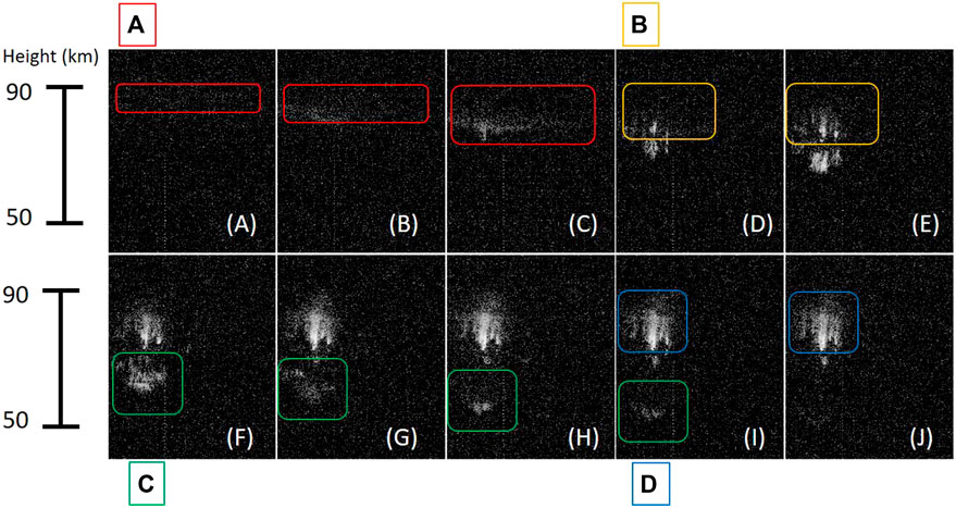
FIGURE 3. Although AP lacks sufficient spatial resolution to point out their development stages, we used typical sprite events in the 2018 Taiwan campaign and extracted the major dynamic features of sprite development. These features of sprite developing stages help us to analyze the AP-measured emission ratio for the ISUAL-recorded sprites events in times and in altitudes, also corresponding to Figures 4 (A–D).

FIGURE 4

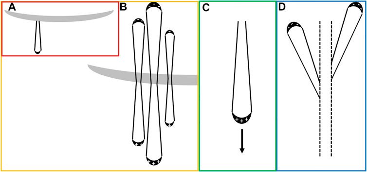
FIGURE 4. To analyze the AP emission characteristics of each developed stage in ISUAL recorded sprites, we choose (A) sprite streamer inception, (B) upper branches of bi-directional streamers with negative polarity, (C) downward propagating streamers with positive polarity, and (D) reigniting of upward streamer in the sprite body for specific streamer process in Figure 3 and later used to study the AP measured emission ratio.

Two Distinct Types of Observed Sprites Determined by Their Inception Altitudes: Sprite Halo Event and the Carrot Sprite Event

Sprites involve streamer heads emerging from the downward leading edge of a halo or plasma inhomogeneity and branching into both downward streamers and upward-propagating streamers simultaneously (Stanley et al., 1999; Stenbaek-Nielsen et al., 2000; Moudry et al., 2003; Marshall and Inan, 2005; Cummer et al., 2006; McHarg et al., 2007; Stenbaek-Nielsen et al., 2013). Numerical studies compared sprite halo and carrot sprites (Qin et al., 2011). The short-delayed halo sprites were possibly produced by a–CG (Cloud-to-Ground lightning with negative polarity) with an impulsive lightning current and without continuing current, while long-delayed carrot sprites were triggered by + CG (Cloud-to-Ground lightning with positive polarity) due to a long-lasting high field region for a lightning continuing current. Listed in Table 1, we selected sprite events from 2005 to 2011 to minimize possible uncertainty in emission ratios. Ten sprite events were excluded from twenty candidates. In six sprite events lightning was more powerful than the AP-measured blue/red emission. Difficulties were faced in another four sprite events in separating the sprite emission from the lightning emission. The final ten selections are included in Table 1 which shows the characteristics of sprite halo and carrot sprite events in their inception altitudes, AP-measured ratios, and emission times.

In ISUAL recorded images (spatial resolution ∼2 km), sprite halos events have narrow structures (likely column sprites) with a distinguished halo. In contrast, carrot sprites have compact structures with higher brightness and longer emission duration. For AP-measured emission altitudes, sprite halo events were accompanied by downwardly-propagating streamers, and were intercepted at altitudes 84.3 ± 3.8 km with an average emission time 0.9 ± 0.3 ms. Otherwise, the AP measured emission for carrot sprite events began at lower altitudes 67.4 ± 7.6 km and developed into upward and downward-propagating emissions with an average emission time 3.0 ± 0.5 ms. Besides, a mixed type was found that a sprite event at time 21:45:48.239 (UT) on Mach 16, 2006 initialized at 83.4 ± 6.8 km with an emission time 2.9 ms, not listed in Table 1. The sprite event has both characteristics of our categorized sprite halos and carrot sprites. We identified this event with the mixed type. The sprite may be accompanied by the halo emission at higher altitudes and finally developed into a whole carrot sprite with a more prolonged emission. The recorded images also show the cloud emission lasted more than 180 ms. We conjecture the sprite event may be affected by the lightning continuing current associated with cloud emissions.

Figure 5 compares two distinct categories of sprite events (sprite halo and carrot sprite events) distinguished by their inception altitudes and their AP-measured emission, listed in Table 1; Figures 6, 7 show their spatial and temporal diagrams of AP-measured blue-to-red ratios, respectively. For a sprite halo event (14:43:37.240 UT on October 3, 2005) Figures 5A, 6A show AP-measured ratios in green cross symbols as referenced by curves to represent the simulated streamer ratios with 0.4–4.6 E_k. Figure 6B indicates the diagram of AP-measured ratios by colors in altitudes and times. In Figure 6B, a sprite halo is initialized at an altitude of 88.5 ± 6.3 km, which corresponds to the altitude range of the transition from a halo to the inception of sprite streamers in Figure 5A. The AP signals propagated down to a lower altitude of 62.6 ± 6.3 km. As shown in Figure 6A, AP-measured ratios (green cross symbols) are found between 0.9 E_k and 3.7–4.6 E_k in the streamer head. Although AP-measured ratios have lower values than predicted emission ratios (thick cyan and magenta lines), the statistical analysis in Figure 8A with more sprite halo events implies that the AP-measured ratios are consistent with predicted emission ratios.

FIGURE 5

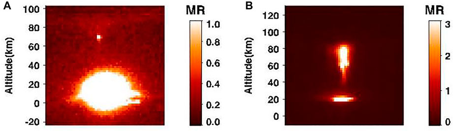
FIGURE 5. Two distinct types of observed sprites determined by the AP where the color indicates the brightness in units of MR (mega Rayleigh): (A) the sprite halo event observed at 14:53:13.687–716 on October 3, 2005 where the upper part (70–90 km) was a funnel-shaped halo structure with a compact sprite emission at ∼ 70 km, and the lower part (0–40 km) was a nut-shaped lightning emission filled with scattered photons (Luque et al., 2020), and (B) the carrot sprite event at 04:36:16.235 (UT) on July 11, 2010. The carrot sprite emission extended widely at altitudes of 30–90 km over the cloud top emission at a projected altitude up to ∼20 km.

FIGURE 6

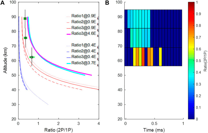
FIGURE 6. The sprite halo event observed at 14:53:13.687–716 on October 3, 2005: (A) the AP-measured ratio 2P/1P with predicted emission ratios of Ratio 1 $\left(r_{CB}\right)$, Ratio 2 $\left(R_{CB}\right)$, and Ratio 3 $\left(R_{CB}^{\ast }\right)$ at ambient electric fields of 0.4 E_k and 0.9 E_k. The thick cyan and magenta lines represent the predicted 2P/1P ratio in sprite streamer simulations with streamer head electric fields of 3.7 E_k and 4.6 E_k under ambient electric fields of 0.4 E_k and 0.9 E_k, respectively. The green crosses indicate the data points of AP-measured ratios, while the square symbols are the means of the AP-measured ratios, and the horizontal bars are their standard deviations. (B) the diagram of AP-measured ratios indicated by colors in altitudes and times.

FIGURE 7

FIGURE 7. The carrot sprite event at 04:36:16.235 (UT) on July 11, 2010: (A) the AP-measured ratio 2P/1P with predicted emission ratios of Ratio 1 $\left(r_{CB}\right)$, Ratio 2 $\left(R_{CB}\right)$, and Ratio 3 $\left(R_{CB}^{\ast }\right)$ at ambient electric fields of 0.4 E_k and 0.9 E_k. The thick cyan and magenta lines represent the predicted 2P/1P ratio in sprite streamer simulations with streamer head electric fields of 3.7 E_k and 4.6 E_k under ambient electric fields of 0.4 E_k and 0.9 E_k, respectively. (B) the diagram of AP-measured ratios indicated by colors in altitude and time.

FIGURE 8

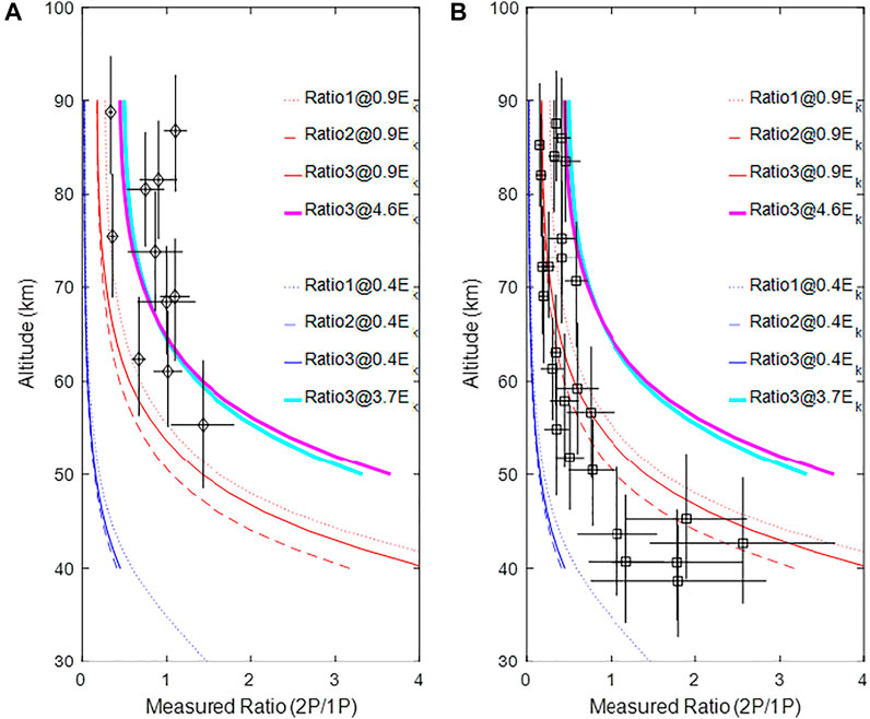
FIGURE 8. AP-measured emission ratios of 2P to 1P for 10 selected sprite events without potential lightning contamination. Two categories of ISUAL sprite events are shown in AP-measured ratios: (A) sprite halo events with impulse AP emission time (0.9 ± 0.3 ms) and higher estimated electric fields, and (B) carrot sprite events with long AP emission time (3.0 ± 0.5 ms) and lower estimated electric fields.

Figure 5B shows a carrot sprite event without a distinguished halo observed at 04:36:16.235 (UT) on July 11, 2010. The AP-measured blue/red emission peaks are delayed about 0.4 ms after the recorded lightning signal by SP5 at 777.4 nm. The carrot sprite event initialized at an estimated altitude of 68.8 ± 6.8 km, and subsequently propagated downwardly and upwardly. Figure 7A compares AP-measured ratios with predicted emission ratios while Figure 7B shows their timing diagram in altitude. The carrot sprite initialized in an altitude range of 62–76 km at time −0.4 ms, and developed into lower altitude emission in the interval −0.4–0.05 ms. Unexpectedly, AP-measured ratios approach the red lines (0.9 E_k). After the time 0.05 ms, AP-measured ratios gradually decreased and reached to the blue lines (0.4 E_k). The gradual decrease of the emission ratios can be understood since the sprite streamer energy is finally dissipated in electron collisions with ambient molecules. In addition, the upper branches of sprite emission occurred after 0 ms where the AP-measured ratios have a maximum value 0.33. Similarly, the AP-measured ratios are slightly higher than red lines (0.9 E_k) and are lower than predicted emissions in cyan and magenta lines (3.7–4.6 E_k). Next, we collected additional sprite events to support more evidence on the higher emission ratios for sprite halos and lower values for carrot sprites.

Statistical Analysis of AP-Measured Emission Ratios

Figure 8 shows the selected sprite events where each event has 3-4 points measured in the corresponding altitude range by the AP vertically-stacked channels. The square symbol indicates the mean sprite ratio at a specified altitude, where the vertical error bars show the altitude range of the AP measurements. The horizontal error bars indicate the standard deviation of the AP-measured ratios in the same AP channels. In Figure 8A, the AP-measured ratios (2P/1P) in sprite halo events have data points scattered around the curves for predicted emission ratios from streamer head electric fields (3.7–4.6 E_k for cyan and magenta lines). The scatter in the distribution of AP measured ratios in sprite halos events of Figure 8A may is attributable to the variances of large-scale quasi-steady electric field magnitudes caused by charge transfer inside the clouds beneath or to uncertainty in the AP measurement with unknown reasons.

In Figure 8B, the carrot sprite events initialized at a lower altitude of 60–75 km, and have lower emission ratios than sprite halos events in Figure 8A. AP-measured ratios are slightly lower than the predicted ratios (streamer head electric fields of 3.7 E_k and 4.6 E_k in cyan and magenta lines) in higher altitudes of 65–90 km (sprite upper branches and central regions). The lower tendrils in carrot sprites at lower altitudes (50–65 km) have increased emission rates. The emission ratios reflect the quenching effect in Analytical expressions for sprite emission ratios. But these values are unexpected, ranging between blue lines (0.4 Ek) and red lines (0.9 E_k) in Figure 8B.

Figure 8B have a lower bound of data points near blue lines (0.4 E_k). Most of the estimated ambient electric fields were greater than 0.4 E_k. The ambient electric field threshold (0.4 E_k) is consistent with the results of remote electromagnetic field measurements for short-delayed or big/bright sprites (Hu et al., 2002; Li et al., 2008). The non-streamer head regions (such as sprite streamers’ bodies and tails or the surroundings of sprite streamers) may contribute additional red (1P) emission, which may cause lower emission ratios (2P/1P). Stenbaek-Nielsen et al. (2020) compared the blue-to-red emission ratio and found that upper propagating streamer, sprite beads, and glow have lower emission ratios. For those non-streamer processes, a large percentage of 1P (red) emission makes lower AP-measured ratios, especially for the case of long emission time in the carrot sprites. Hence, for carrot sprites, our study shows that sprite inception at lower altitudes may favor development into the whole complex structures of sprites, which may be accompanied by non-streamer emission or sprite beads caused by attachment instability in streamer channels (Luque et al., 2016). The Possibly a pre-existing free ionized plasma patch in the early stage of sprites may provide more free energized electrons. More non-streamer processes with lower emission ratios could occur and co-exist with reigniting of upward streamers. Next, we provide an example case to show the effect of a favorable plasma environment.

The Effects of AP-Measured Ratios for a Pre-existing Sprite on a Later-Occurring Sprite

Figure 9 shows successive sprite events at 22:01:23.178 (UT) on August 3, 2007, which are also called dancing sprites (Lyons, 1994; Bór et al., 2018 and reference therein). The preceding sprite event in Figure 9A began ∼85 ms before the second sprite event with lower brightness in Figure 9B. We also demonstrate the decrease in emission ratios for a pre-existing sprite on a later-occurring sprite in Figures 10, 11. The measured emission ratios for the pre-existing sprite and the later-occurring sprite are compared with predicted emission ratios Ratio 1 $\left(r_{CB}\right)$, Ratio 2 $\left(R_{CB}\right)$, and Ratio 3 $\left(R_{CB}^{\ast }\right)$.

FIGURE 9

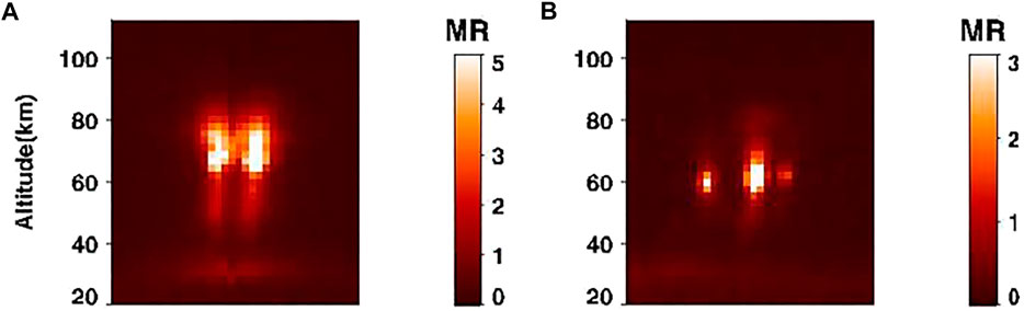
FIGURE 9. Successive sprite events at 22:01:23.178 (UT) from August 3, 2007, demonstrating the effects of AP-measured emission ratios for (A) a pre-existing sprite and, (B) a later-occurring sprite, which are also called dancing sprites.

FIGURE 10

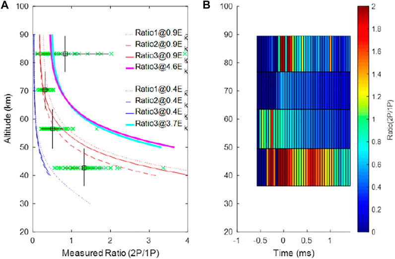
FIGURE 10. The (A) AP-measured ratio 2P/1P with predicted emission ratios and (B) the diagram of AP-measured ratios indicated by colors in altitudes and times for the pre-existing sprite event at 22:01:23.178 (UT) from August 3, 2007.

FIGURE 11

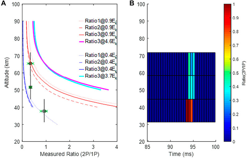
FIGURE 11. The (A) the AP-measured ratio 2P/1P with predicted emission ratios and (B) the diagram of AP-measured ratios indicated by colors in altitude and time for the later-occurring sprite event at 22:01:23.178 (UT) from August 3, 2007.

The comparison of Figure 10A with Figure 11A shows a slightly lower value of AP-measured emission ratio 2P/1P, which may imply that the plasma environment and the generation mechanism of the second sprite event may be different from that of the first sprite event. Successive sprite events have been reported in previous studies using a high-speed image-intensified camera (Stenbaek-Nielsen et al., 2000). A second sprite occurred in the fading region of the first sprite, gradually brightened, and developed branched tendrils towards lower altitudes. The upwardly branched streamers may arise from previous older streamer channels (Stenbaek-Nielsen et al., 2000; Luque et al., 2016). The AP-measured emission ratio in Figure 11B provides direct evidence of the upper branches developing in pre-existing sprite structures where lower-altitude AP-measured ratios developed into the region at higher altitude. The AP-measured ratios in the later-occurring sprite are lower than that in the previous sprite event. That may support the idea that the change of the plasma environment may cause lower emission ratios in carrot sprite events.

Summary

We verified experimentally the AP-measured emission ratio 2P/1P and compared it with the theoretically predicted sprite emission ratio 2P/1P using numerical results on sprite streamers (Celestin and Pasko, 2010; Pérez-Invernón et al., 2018). AP-measured ratios in sprite halo events are consistent with predicted ratios for streamer head electric fields of 3.7 E_k and 4.6 E_k in Figure 8A. Most carrot sprite events initialized at altitudes 67.4 ± 7.6 km with lower estimated electric field 1∼3 or 4 E_k. Below 60 km, surprisingly, AP-measured ratios fell below the predicted ratio 1 E_k. We conjectured that the lower emission ratios are contributed from those non-streamer regions (upper propagating streamer, sprite beads, and glow) by Stenbaek-Nielsen et al. (2020). In addition, the AP-measured ratios have a lower bound of predicted emission ratios associated with 0.4 E_k.

For space-based optical diagnostics in limb observation, as with the ISUAL mission, the main conclusions from our studies on the sprite emission ratio 2P/1P are the following:

1) For accurate analyses of ISUAL AP data, we selected sprite events from the first 7 years (2004–2011) of operation to avoid the degradation in instrument performance. After analyzing the ten selected sprite events, the AP-measured ratios scatter widely as previous results in sprites (Adachi et al., 2008), and estimated electric fields range between 0.4 E_k and greater than 4 E_k. The downward propagating streamers verified the streamer head electric fields in the range ∼3.7–4.6 E_k. At lower altitudes, AP-measured ratios have a lower bound, corresponding to the predicted ratio for 0.4 E_k. The threshold of the estimated electric field (0.4 E_k) is consistent with the earlier results of remote electromagnetic field measurements for short-delayed or big/bright sprites (Hu et al., 2002; Li et al., 2008).

2) The AP-measured ratios of downward propagating streamers in sprite halo events scattered around the ratios predicted by numerical streamer head electric fields with 3.7–4.6 E_k (Ihaddadene and Celestin, 2017) where the estimated electric field was in the range 0.4–∼0.9 E_k. However, for carrot sprite events, the AP-measured emission ratio 2P/1P showed lower values than predicted ratios. The extra 1P red emission may be contributed from non-streamer dominant emissions: sprite beads and glow or possibly by plasma environment changes in upper streamers in carrot sprites with lower inception altitude and longer emission time Qin et al., 2014.

Data Availability Statement

The original contributions presented in the study are included in the article/Supplementary Material, and further inquiries can be directed to the corresponding author.

Author Contributions

EW conceived the study to check AP data for sprite halos. C-LK analyzed AP data. KI and SC formulated the analytical equations for sprite emission ratios and conducted the simulation of sprite streamers. TA, YT, HF, and SM provided the AP calibration data. YT, HF, SM, R-RH, and L-CL were all part of the ISUAL science team. All authors contributed to the final interpretation and writing of the manuscript with major contribution by C-LK.

Funding

The work of C-LK was supported in part by grants MOST 110-2111-M-008-007, MOST 109-2111-M-008-006 and MOST 108-2111-M-008-005 from Ministry of Science and Technology of Taiwan.

Conflict of Interest

The authors declare that the research was conducted in the absence of any commercial or financial relationships that could be construed as a potential conflict of interest.

Publisher’s Note

All claims expressed in this article are solely those of the authors and do not necessarily represent those of their affiliated organizations, or those of the publisher, the editors and the reviewers. Any product that may be evaluated in this article, or claim that may be made by its manufacturer, is not guaranteed or endorsed by the publisher.

Acknowledgments

We benefitted from the preliminary studies by Master student Mr. Pei-Yu Chen, and appreciate the assistance and support from the staff at the Center for Astronautical Physics and Engineering of National Central University in Taiwan.

References

Adachi, T., Fukunishi, H., Takahashi, Y., Hiraki, Y., Hsu, R.-R., Su, H.-T., et al. (2006). Electric Field Transition between the Diffuse and Streamer Regions of Sprites Estimated from ISUAL/array Photometer Measurements. Geophys. Res. Lett. 33, 17803. doi:10.1029/2006GL026495

CrossRef Full Text | Google Scholar

Adachi, T., Hiraki, Y., Yamamoto, K., Takahashi, Y., Fukunishi, H., Hsu, R.-R., et al. (2008). Electric fields and Electron Energies in Sprites and Temporal Evolutions of Lightning Charge Moment. J. Phys. D: Appl. Phys. 41 (23), 234010. doi:10.1088/0022-3727/41/23/234010

CrossRef Full Text | Google Scholar

Armstrong, R. A., Shorter, J. A., Taylor, M. J., Suszcynsky, D. M., Lyons, W. A., and Jeong, L. S. (1998). Photometric Measurements in the SPRITES '95 & '96 Campaigns of Nitrogen Second Positive (399.8 Nm) and First Negative (427.8 Nm) Emissions. J. Atmos. Solar‐Terrestrial Phys. 60 (7–9), 787–799. doi:10.1016/S1364‐6826(98)00026‐1

CrossRef Full Text | Google Scholar

Armstrong, R. A., Suszcynsky, D. M., Lyons, W. A., and Nelson, T. E. (2000). Multi-color Photometric Measurements of Ionization and Energies in Sprites. Geophys. Res. Lett. 27 (5), 653–656. doi:10.1029/1999GL003672

CrossRef Full Text | Google Scholar

Babaeva, N. Y., and Naidis, G. V. (1997). Dynamics of Positive and Negative Streamers in Air in Weak Uniform Electric fields. IEEE Trans. Plasma Sci. 25, 375–379. doi:10.1109/27.602514

CrossRef Full Text | Google Scholar

Barrington-Leigh, C. P., and Inan, U. S. (1999). Elves Triggered by Positive and Negative Lightning Discharges. Geophys. Res. Lett. 26, 683–686. doi:10.1029/1999gl900059

CrossRef Full Text | Google Scholar

Bór, J., Zelkó, Z., Hegedüs, T., Jäger, Z., Mlynarczyk, J., Popek, M., et al. (2018). On the Series of +CG Lightning Strokes in Dancing Sprite Events. J. Geophys. Res. Atmos. 123, 11030–11047. doi:10.1029/2017JD028251

CrossRef Full Text | Google Scholar

Celestin, S., and Pasko, V. P. (2010). Effects of Spatial Non-uniformity of Streamer Discharges on Spectroscopic Diagnostics of Peak Electric fields in Transient Luminous Events. Geophys. Res. Lett. 37 (7), a–n. doi:10.1029/2010GL042675

CrossRef Full Text | Google Scholar

Chern, J. L., Hsu, R. R., Su, H. T., Mende, S. B., Fukunishi, H., Takahashi, Y., et al. (2003). Global Survey of Upper Atmospheric Transient Luminous Events on the ROCSAT-2 Satellite. J. Atmos. Solar-Terrestrial Phys. 65, 647–659. doi:10.1016/S1364-6826(02)00317-6

CrossRef Full Text | Google Scholar

Cummer, S. A., Jaugey, N., Li, J., Lyons, W. A., Nelson, T. E., and Gerken, E. A. (2006). Submillisecond Imaging of Sprite Development and Structure. Geophys. Res. Lett. 33 (4). doi:10.1029/2005gl024969

CrossRef Full Text | Google Scholar

Frey, H. U., Mende, S. B., Harris, S. E., Heetderks, H., Takahashi, Y., Su, H. T., et al. (2016). The Imager for Sprites and Upper Atmospheric Lightning (ISUAL). J. Geophys. Res. Space Phys. 121 (8), 8134–8145. doi:10.1002/2016JA022616

CrossRef Full Text | Google Scholar

Gordillo-Vázquez, F. J., Luque, A., and Simek, M. (2012). Near Infrared and Ultraviolet Spectra of TLEs. J. Geophys. Res. 117, a–n. doi:10.1029/2012JA017516

CrossRef Full Text | Google Scholar

Gordillo-Vázquez, F. J., and Pérez-Invernón, F. J. (2021). A Review of the Impact of Transient Luminous Events on the Atmospheric Chemistry: Past, Present, and Future. Atmos. Res. 252, 105432. doi:10.1016/j.atmosres.2020.105432

CrossRef Full Text | Google Scholar

Green, B. D., Fraser, M. E., Rawlins, W. T., Jeong, L., Blumberg, W. A. M., Mende, S. B., et al. (1996). Molecular Excitation in Sprites. Geophys. Res. Lett. 23 (16), 2161–2164. doi:10.1029/96GL02071

CrossRef Full Text | Google Scholar

Hampton, D. L., Heavner, M. J., Wescott, E. M., and Sentman, D. D. (1996). Optical Spectral Characteristics of Sprites. Geophys. Res. Lett. 23 (1), 89–92. doi:10.1029/95GL03587

CrossRef Full Text | Google Scholar

Hu, W., Cummer, S. A., Lyons, W. A., and Nelson, T. E. (2002). Lightning Charge Moment Changes for the Initiation of Sprites. Geophys. Res. Lett. 29 (8), 120–124. doi:10.1029/2001gl014593

CrossRef Full Text | Google Scholar

Ihaddadene, M. A., and Celestin, S. (2017). Determination of Sprite Streamers Altitude Based on N 2 Spectroscopic Analysis. J. Geophys. Res. Space Phys. 122 (1), 1000–1014. doi:10.1002/2016ja023111

CrossRef Full Text | Google Scholar

Kanmae, T., Stenbaek-Nielsen, H. C., McHarg, M. G., and Haaland, R. K. (2010b). Observation of Blue Sprite Spectra at 10,000 Fps. Geophys. Res. Lett. 37, a–n. doi:10.1029/2010GL043739

CrossRef Full Text | Google Scholar

Kanmae, T., Stenbaek-Nielsen, H. C., McHarg, M. G., and Haaland, R. K. (2010a). Observation of Sprite Streamer Head's Spectra at 10,000 Fps. J. Geophys. Res. 115, A00E48. doi:10.1029/2009JA014546

CrossRef Full Text | Google Scholar

Kosar, B. C., Liu, N., and Rassoul, H. K. (2012). Luminosity and Propagation Characteristics of Sprite Streamers Initiated from Small Ionospheric Disturbances at Subbreakdown Conditions. J. Geophys. Res. 117 (A8), a–n. doi:10.1029/2012ja017632

CrossRef Full Text | Google Scholar

Kuo, C.-L., Chou, J. K., Tsai, L. Y., Chen, A. B., Su, H. T., Hsu, R. R., et al. (2009). Discharge Processes, Electric Field, and Electron Energy in ISUAL-Recorded Gigantic Jets. J. Geophys. Res. 114 (A4), a–n. doi:10.1029/2008ja013791

CrossRef Full Text | Google Scholar

Kuo, C.-L., Hsu, R. R., Chen, A. B., Su, H. T., Lee, L. C., Mende, S. B., et al. (2005). Electric fields and Electron Energies Inferred from the ISUAL Recorded Sprites. Geophys. Res. Lett. 32, a–n. doi:10.1029/2005GL023389

CrossRef Full Text | Google Scholar

Kuo, C. L., Chen, A. B., Chou, J. K., Tsai, L. Y., Hsu, R. R., Su, H. T., et al. (2008). Radiative Emission and Energy Deposition in Transient Luminous Events. J. Phys. D: Appl. Phys. 41, 234014. doi:10.1088/0022-3727/41/23/234014

CrossRef Full Text | Google Scholar

Li, J., Cummer, S. A., Lyons, W. A., and Nelson, T. E. (2008). Coordinated Analysis of Delayed Sprites with High-Speed Images and Remote Electromagnetic fields. J. Geophys. Res. 113 (D20), 77. doi:10.1029/2008jd010008

CrossRef Full Text | Google Scholar

Liu, N., Pasko, V. P., Burkhardt, D. H., Frey, H. U., Mende, S. B., Su, H.-T., et al. (2006). Comparison of Results from Sprite Streamer Modeling with Spectrophotometric Measurements by ISUAL Instrument on FORMOSAT-2 Satellite. Geophys. Res. Lett. 33 (1), a–n. doi:10.1029/2005GL024243

CrossRef Full Text | Google Scholar

Liu, N., and Pasko, V. P. (2004). Effects of Photoionization on Propagation and Branching of Positive and Negative Streamers in Sprites. J. Geophys. Res. 109, A04301. doi:10.1029/2003JA010064

CrossRef Full Text | Google Scholar

Liu, N. Y., Pasko, V. P., Adams, K., Stenbaek-Nielsen, H. C., and McHarg, M. G. (2009). Comparison of Acceleration, Expansion, and Brightness of Sprite Streamers Obtained from Modeling and High-Speed Video Observations. J. Geophys. Res. 114 (A3), a–n. doi:10.1029/2008ja013720

CrossRef Full Text | Google Scholar

Luque, A., Gordillo-Vázquez, F. J., Li, D., Malagón-Romero, A., Pérez-Invernón, F. J., Schmalzried, A., et al. (2020). Modeling Lightning Observations from Space-Based Platforms (CloudScat.Jl 1.0). Geosci. Model. Dev. 13 (11), 5549–5566. doi:10.5194/gmd-13-5549-2020

CrossRef Full Text | Google Scholar

Luque, A., Stenbaek-Nielsen, H. C., McHarg, M. G., and Haaland, R. K. (2016). Sprite Beads and Glows Arising from the Attachment Instability in Streamer Channels. J. Geophys. Res. Space Phys. 121 (3), 2431–2449. doi:10.1002/2015ja022234

CrossRef Full Text | Google Scholar

Lyons, W. A. (1994). Characteristics of Luminous Structures in the Stratosphere above Thunderstorms as Imaged by Low-Light Video. Geophys. Res. Lett. 21 (10), 875–878. doi:10.1029/94GL00560

CrossRef Full Text | Google Scholar

Marshall, R. A., and Inan, U. S. (2005). High-speed Telescopic Imaging of Sprites. Geophys. Res. Lett. 32 (5). doi:10.1029/2004gl021988

CrossRef Full Text | Google Scholar

McHarg, M. G., Stenbaek-Nielsen, H. C., and Kammae, T. (2007). Observations of Streamer Formation in Sprites. Geophys. Res. Lett. 34, 06804. doi:10.1029/2006GL027854

CrossRef Full Text | Google Scholar

Mende, S. B., Frey, H. U., Hsu, R. R., Su, H. T., Chen, A. B., Lee, L. C., et al. (2005). Dregion Ionization by Lightning-Induced Electromagnetic Pulses. J. Geophys. Res. 110, 11312. doi:10.1029/2005JA011064

CrossRef Full Text | Google Scholar

Mende, S. B., Rairden, R. L., Swenson, G. R., and Lyons, W. A. (1995). Sprite Spectra; N21 PG Band Identificationfication. Geophys. Res. Lett. 22 (19), 2633–2636. doi:10.1029/95GL02827

CrossRef Full Text | Google Scholar

Miyasato, R., Fukunishi, H., Takahashi, Y., and Taylor, M. J. (2003). Energy Estimation of Electrons Producing Sprite Halos Using Array Photometer Data. J. Atmos. Solar-Terrestrial Phys. 65, 573–581. doi:10.1016/s1364-6826(02)00322-x

CrossRef Full Text | Google Scholar

Miyasato, R., Taylor, M. J., Fukunishi, H., and Stenbaek-Nielsen, H. C. (2002). Statistical Characteristics of Sprite Halo Events Using Coincident Photometric and Imaging Data. Geophys. Res. Lett. 29 (21), 2033. doi:10.1029/2001GL014480

CrossRef Full Text | Google Scholar

Morrill, J., Bucsela, E., Siefring, C., Heavner, M., Berg, S., Moudry, D., et al. (2002). Electron Energy and Electric Field Estimates in Sprites Derived from Ionized and neutralN2emissions. Geophys. Res. Lett. 29 (10), 100–104. doi:10.1029/2001gl014018

CrossRef Full Text | Google Scholar

Moss, G. D., Pasko, V. P., Liu, N., and Veronis, G. (2006). Monte Carlo Model for Analysis of thermal Runaway Electrons in Streamer Tips in Transient Luminous Events and Streamer Zones of Lightning Leaders. J. Geophys. Res. 111 (A2). doi:10.1029/2005ja011350

CrossRef Full Text | Google Scholar

Moudry, D., Stenbaek-Nielsen, H., Sentman, D., and Wescott, E. (2003). Imaging of Elves, Halos and Sprite Initiation at Time Resolution. J. Atmos. Solar-Terrestrial Phys. 65, 509–518. doi:10.1016/s1364-6826(02)00323-1

CrossRef Full Text | Google Scholar

Pasko, V. P., Inan, U. S., and Bell, T. F. (1998). Spatial Structure of Sprites. Geophys. Res. Lett. 25 (12), 2123–2126. doi:10.1029/98gl01242

CrossRef Full Text | Google Scholar

Pasko, V. P., Inan, U. S., Bell, T. F., and Taranenko, Y. N. (1997). Sprites Produced by Quasi-Electrostatic Heating and Ionization in the Lower Ionosphere. J. Geophys. Res. 102 (A3), 4529–4561. doi:10.1029/96ja03528

CrossRef Full Text | Google Scholar

Pérez‐Invernón, F. J., Luque, A., Gordillo‐Vázquez, F. J., Sato, M., Ushio, T., Adachi, T., et al. (2018). Spectroscopic Diagnostic of Halos and Elves Detected from Space‐Based Photometers. J. Geophys. Res. Atmos. 123 (22), 912917–912941. doi:10.1029/2018jd029053

CrossRef Full Text | Google Scholar

Qin, J., Celestin, S., and Pasko, V. P. (2011). On the Inception of Streamers from Sprite Halo Events Produced by Lightning Discharges with Positive and Negative Polarity. J. Geophys. Res. 116, a–n. doi:10.1029/2010JA016366

CrossRef Full Text | Google Scholar

Qin, J., Pasko, V. P., McHarg, M. G., and Stenbaek-Nielsen, H. C. (2014). Plasma Irregularities in the D-Region Ionosphere in Association with Sprite Streamer Initiation. Nat. Commun. 5, 3740. doi:10.1038/ncomms4740

PubMed Abstract | CrossRef Full Text | Google Scholar

Sentman, D. D., Wescott, E. M., Osborne, D. L., Hampton, D. L., and Heavner, M. J. (1995). Preliminary Results from the Sprites94 Aircraft Campaign: 1. Red Sprites. Geophys. Res. Lett. 22 (10), 1205–1208. doi:10.1029/95GL00583

CrossRef Full Text | Google Scholar

Stanley, M., Krehbiel, P., Brook, M., Moore, C., Rison, W., and Abrahams, B. (1999). High Speed Video of Initial Sprite Development. Geophys. Res. Lett. 26 (20), 3201–3204. doi:10.1029/1999gl010673

CrossRef Full Text | Google Scholar

Stenbaek‐Nielsen, H. C., McHarg, M. G., Haaland, R., and Luque, A. (2020). Optical Spectra of Small‐Scale Sprite Features Observed at 10,000 Fps. J. Geophys. Res. Atmos. 125, e2020JD033170. doi:10.1029/2020JD033170

CrossRef Full Text | Google Scholar

Stenbaek-Nielsen, H. C., Kanmae, T., McHarg, M. G., and Haaland, R. (2013). High-Speed Observations of Sprite Streamers. Surv. Geophys. 34, 769–795. doi:10.1007/s10712-013-9224-4

CrossRef Full Text | Google Scholar

Stenbaek-Nielsen, H. C., Moudry, D. R., Wescott, E. M., Sentman, D. D., and Sabbas, F. T. S. (2000). Sprites and Possible Mesospheric Effects. Geophys. Res. Lett. 27 (23), 3829–3832. doi:10.1029/2000gl003827

CrossRef Full Text | Google Scholar

Wescott, E. M., Stenbaek-Nielsen, H. C., Sentman, D. D., Heavner, M. J., Moudry, D. R., and Sabbas, F. T. S. (2001). Triangulation of Sprites, Associated Halos and Their Possible Relation to Causative Lightning and Micrometeors. J. Geophys. Res. 106 (A6), 10467–10477. doi:10.1029/2000JA000182

CrossRef Full Text | Google Scholar

Wu, Y. J., Williams, E., Chang, S. C., Chou, J. K., Hsu, R. R., Friedrich, M., et al. (2017). The Leading Role of Atomic Oxygen in the Collocation of Elves and Hydroxyl Nightglow in the Low-Latitude Mesosphere. J. Geophys. Res. Space Phys. 122 (5), 5550–5567. doi:10.1002/2016JA023681

CrossRef Full Text | Google Scholar