 B. B. T. Wassing
 T. Candela
 S. Osinga
 P. A. Fokker
95% of researchers rate our articles as excellent or good
Learn more about the work of our research integrity team to safeguard the quality of each article we publish.
Find out more
ORIGINAL RESEARCH article
Front. Earth Sci. , 14 September 2021
Sec. Geohazards and Georisks
Volume 9 - 2021 | https://doi.org/10.3389/feart.2021.685841
This article is part of the Research Topic Advances in Monitoring, Modeling and Managing Induced Seismicity View all 11 articles
This paper describes and deploys a workflow to assess the evolution of seismicity associated to injection of cold fluids close to a fault. We employ a coupled numerical thermo-hydro-mechanical simulator to simulate the evolution of pressures, temperatures and stress on the fault. Adopting rate-and-state seismicity theory we assess induced seismicity rates from stressing rates at the fault. Seismicity rates are then used to derive the time-dependent frequency-magnitude distribution of seismic events. We model the seismic response of a fault in a highly fractured and a sparsely fractured carbonate reservoir. Injection of fluids into the reservoir causes cooling of the reservoir, thermal compaction and thermal stresses. The evolution of seismicity during injection is non-stationary: we observe an ongoing increase of the fault area that is critically stressed as the cooling front propagates from the injection well into the reservoir. During later stages, models show the development of an aseismic area surrounded by an expanding ring of high seismicity rates at the edge of the cooling zone. This ring can be related to the “passage” of the cooling front. We show the seismic response of the fault, in terms of the timing of elevated seismicity and seismic moment release, depends on the fracture density, as it affects the temperature decrease in the rock volume and thermo-elastic stress change on the fault. The dense fracture network results in a steeper thermal front which promotes stress arching, and leads to locally and temporarily high Coulomb stressing and seismicity rates. We derive frequency-magnitude distributions and seismic moment release for a low-stress subsurface and a tectonically active area with initially critically stressed faults. The evolution of seismicity in the low-stress environment depends on the dimensions of the fault area that is perturbed by the stress changes. The probability of larger earthquakes and the associated seismic risk are thus reduced in low-stress environments. For both stress environments, the total seismic moment release is largest for the densely spaced fracture network. Also, it occurs at an earlier stage of the injection period: the release is more gradually spread in time and space for the widely spaced fracture network.
The role of geothermal energy production in the global energy supply is expected to grow (IEA, 2020), as the energy transition requires a shift from fossil-fuel based to renewable and sustainable energy sources. Geothermal energy can be produced from high-enthalpy geothermal fields, but also low-enthalpy sedimentary formations such as found in intraplate regions like e.g. the Netherlands. In the last 2 decades, over 20 low enthalpy geothermal doublet production systems have been successfully developed in the Netherlands (e.g. Van Wees et al., 2020). The majority of these doublets target porous sandstone reservoirs of Permian to Cretaceous age (Buijze et al., 2019). However, the increased demand for sustainable heat and electricity calls for a broadening of the geological targets for geothermal energy. Therefore, exploration efforts now also target the potential of the Lower Carboniferous Dinantian play in the Netherlands (e.g. Bouroullec et al., 2019; Ter Heege et al., 2020). These Dinantian carbonates typically show heterogeneous porosity and permeability due to the presence of karstification and fractures, as well as relatively high rock competence. The deeper reservoirs among them, which are mainly located in the northern part of the Netherlands, show high in-situ reservoir temperatures up to 190°C (e.g. Lipsey et al., 2016). Consequently, the expected difference between the re-injection temperature and ambient rock temperature is large. The shallower reservoirs in the southeastern part of the Netherlands lie in the Ruhr Valley Graben, a tectonically active region. The full set of reservoir characteristics–tectonic setting, depth, in-situ temperatures, rock competence, poro-perm distribution and the presence or absence of fractures–will affect flow, heat transport and geomechanical response and thereby the seismicity potential of these geothermal plays. Generally speaking, the induced seismicity potential of the Dinantian fractured carbonates is considered to be higher than for the “conventional” sandstone reservoirs (Buijze et al., 2019). Induced earthquakes of magnitudes large enough to be felt at the surface can pose a problem for geothermal doublet operations.
In the southeast of the Netherlands, two geothermal doublets have been operated in carbonate reservoirs of the Dinantian. In contrast to the geothermal doublets producing from porous sandstone reservoirs, where no induced seismicity has been reported to date, some small seismic events have been recorded in the Dinantian reservoirs (Baisch and Vörös, 2018; Vörös and Baisch, 2019). This led to the cessation of the geothermal doublet operations. Recent research points towards a causal relation between operations in the Dinantian carbonates and seismic events (Baisch and Vörös, 2018; Vörös and Baisch, 2019). However, unambiguous conclusions on the relation between subsurface operations and causal mechanisms of induced events were hampered by lack of available data from the subsurface, as well as significant uncertainties in seismic event depth (State Supervision of Mines, 2019). This calls for an improved understanding of the driving mechanisms of induced seismicity in these carbonate reservoirs.
Simulation models capable to assess the potential of fault reactivation and seismicity are crucial to understand the interplay between the operational factors and the evolution of pressures, temperatures and associated changes in the stress fields near geothermal systems (i.e. Wassing et al., 2014; Candela et al., 2018; Van Wees et al., 2020; Wassing et al., 2021). Such models take into account pressure and temperature changes prompted by the production of warm water and re-injection of cooled water which cause changes in stresses in the geothermal reservoir. These may lead to fault reactivation and induced seismicity. Effects of temperature changes on the short term are expected to be limited to the near-well area. However, most geothermal doublets will operate over long periods, up to lifetimes of 50 years. Extensive cooling of the reservoir rocks and the associated stress changes may play a significant role in fault reactivation. Moreover, thermo-elastic stresses may dominate over poro-elastic stress changes and pressure changes, since injection pressures in the carbonate reservoirs are relatively low and thermal stresses can be significant in particular in stiff rocks (e.g. Jacquey et al., 2015). The potential for pressure- or thermally induced seismicity depends on reservoir characteristics, operational conditions and flow rates during geothermal production. Gan and Elsworth (2014) investigated the propagation of fluid pressures and thermal stresses in a prototypical geothermal doublet in a fractured reservoir, and demonstrated that the likelihood for late-stage thermally-induced seismicity depends on the shape of the thermal front.
In the present paper, we focus on seismicity induced by geothermal operations in fractured carbonate reservoirs, such as the Dinantian carbonates in the Netherlands. Using a numerical 3D coupled thermo-hydro-mechanical model (following and extending the method of Gan and Elsworth, 2014), in combination with Dieterich’s rate-and-state-theory (Dieterich, 1994; Segall and Lu, 2015), we investigate and discuss the nucleation of seismicity and the spatial and temporal pattern of seismicity–the “seismic footprint.”
We employ the coupled numerical thermo-hydro-mechanical simulator of FLAC3D-TOUGHREACT (Taron and Elsworth, 2010; Gan and Elsworth, 2014; Wassing et al., 2021). The simulator accounts for the two-way coupling between the thermal, hydraulic and mechanical processes, and provides the spatial and temporal evolution of pore pressures, temperatures and stresses in the model domain. For the present analysis, we do not use the chemical options available in the TOUGHREACT part of the coupled code.
We use a simplified model geometry and modelled pressure, temperature and stress changes due to fluid injection into a single well close to a fault plane. For computational efficiency, we model a quarter of a symmetrical reservoir with a single vertical injection well. Our workflow can easily be extended to model the geometry and configuration of a typical geothermal doublet. Model dimensions are 2,500 × 2500 × 2,100 m. The stress evolution can be computed at any location in the reservoir, over- and underburden. The fault plane itself is not explicitly modelled. We are therefore flexible in choosing the location and orientation of the fault, as there is no need for model remeshing. We define a fault without offset, striking N-S and dipping 70° towards the injection well at a distance of approximately 300 m from the injection well (see Figure 1). Pressures in the fault and stress conditions at the location of the fault plane are derived from 3D interpolation of fracture pressure and stress at the center of the mesh elements.
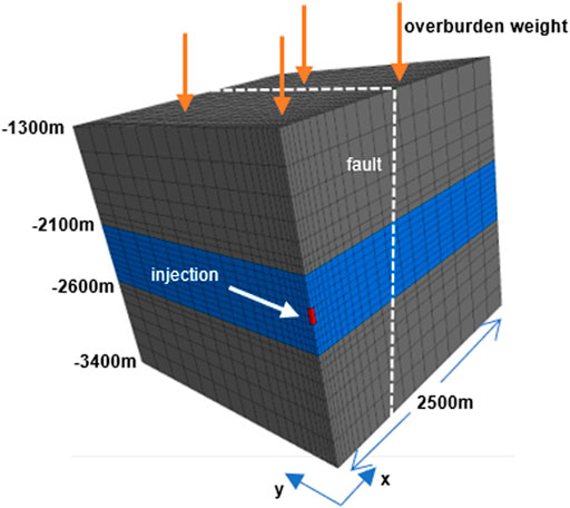
FIGURE 1. Geometry of the model in FLAC3D-TOUGHREACT. Blue color indicates the carbonate reservoir. Red interval depicts injection interval, dashed white line shows position of fault plane, which intersects reservoir and surrounding rocks.
We model the seismic response of a fault in a fractured carbonate reservoir. The top of the reservoir is located at a depth of −2,100 m. Initial reservoir temperature is 90°C. Depth, in-situ temperature, hydrological and thermal parameters of the reservoir are representative of the Dinantian carbonate reservoirs as reported in Ter Heege et al., 2020. The carbonate reservoir itself is relatively thick, 500 m; the fluid is assumed to be injected in an open hole section of 100 m at the center of the reservoir at a depth between −2,300 m and −2,400 m. Fracture sets in the reservoir are modelled as orthogonal with equal spacing and permeability, using the double porosity-permeability approach in TOUGHREACT (Pruess et al., 2012). We distinguish two end-members for the fracture spacing: a small fracture spacing of 2 m and a large fracture spacing of 200 m.
We assume elastic isotropic material behaviour for the reservoir and burden. Elastic properties are uniform throughout the model (see Table 1).
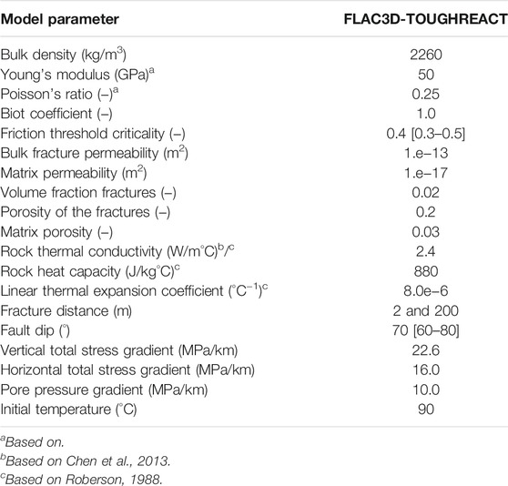
TABLE 1. Model parameters and model ranges for FLAC3D-TOUGHREACT. Values between square brackets indicate a stochastic range of input parameters (uniform distribution).
Initial stress gradients are chosen to be representative of the in-situ stress field in the Netherlands, i.e., an extensional tectonic setting, with little anisotropy in the horizontal stresses (Sv > SHmax = Shmin, respectively −22.6, −16.0, and −16.0 MPa/km). In our model, the minimum horizontal stress is oriented perpendicular to the strike of the fault (parallel to the model x-axis), and maximum horizontal stress is oriented parallel to the fault strike (y-axis). In all modelled cases we assume a hydrostatic pressure gradient. As a result, the initial slip tendency of the fault, defined as the ratio of shear (τs) over effective stress (σ′n) is non-critical with a value | τs/σ′n | ≈ 0.3 at the start of injection. We use the convention that compressive stress is negative.
Cold fluid is injected into the quarter of the injection well at a temperature of 25°C, at a constant rate of 50 kg/s over an open hole section of 100 m. We only model flow and heat transfer in the reservoir section; no flow or thermal conduction into the seal and base rock is modelled. As boundary conditions for flow and heat transport, we impose constant pressure and temperature at the far field vertical boundaries, 2,500 m from the injection well. We assume no displacements in the horizontal direction at the vertical boundaries. For the horizontal boundary at the top and bottom we impose a constant stress, to simulate the weight of the overburden and initial stress equilibrium at depth. The stress response associated to the change of pressure and temperature is computed for the entire model, including the under- and overburden rocks.
Mechanical, thermal and hydrological model parameters and initial conditions and assumptions for the TOUGHREACT-FLAC3D simulations are summarized in Table 1.
As a first step we compute effective normal and shear stresses from the stress tensor at the location of the fault plane. From these we derive the Coulomb stress changes on the fault. Coulomb stress change on a fault is an important proxy for seismicity potential. It is defined by the change of the vertical distance of the effective normal and shear stress to the Mohr-Coulomb failure line in a Mohr diagram. The Coulomb stress changes then result from two contributions. The first is the increase in pore pressures in the fault itself, due to diffusion of pressures through the fracture network (fracture pressure P1) into the fault (so-called “direct pore pressure effect”). The second is the combination of poroelastic and thermoelastic stress changes, caused by the deformation of the rocks due to pressure changes in the fractures (P1) and matrix (P2), respectively temperature changes in the matrix rocks (T2). The Coulomb stress changes are written as:
where the symbol Δ denotes a change, τs is shear stress, σn is total normal stress on the fault, µ is friction coefficient of the fault and
From the evolution of Coulomb stress changes over time we derive Coulomb stressing rates. In turn, the stressing rates are used as input to the rate-and-state seismicity theory originally proposed by Dieterich (1994) to derive seismicity rate (see also Segall and Lu, 2015; Heimisson and Segall, 2018; Candela et al., 2019). Seismicity rates are calculated as:
where the Coulomb stressing rate is defined as:
with
In our model workflow, the Dieterich parameters A,
We refer to Segall and Lu (2015) for a more in-depth discussion of the theory and the parameters involved.
Fault material behaviour is assumed to be fully elastic (i.e. no explicit slip and associated stress redistribution is modelled). To prevent the increase of shear stress and normal effective stress far beyond a realistic failure envelope for shear and tensile strength, we apply corrections for effective normal stress
• if
• if | τs/σ′n | > 1 → | τs/σ′n | = 1
Based on the spatial and temporal evolution of Coulomb stresses and relative seismicity rates we estimate the time-dependent frequency-magnitude distribution of the simulated seismicity at the fault plane near the injector well.
Here we can distinguish two end members: 1) injection in a so-called “low-stress” environment (Segall and Lu, 2015; Maurer and Segall, 2018) and 2) injection in a tectonically active “high-stress” environment. In a high-stress environment, once an event nucleates, it can potentially propagate over the entire fault plane. In a low-stress environment nucleation and propagation of seismic events is assumed to be restricted by the size of the fault segment that is critically stressed (i.e. there will be no run-away rupture outside this perturbed fault segment). In our approach, we use a critical value of shear-over effective normal stress to distinguish between critically and non-critically stressed fault area. In the low-stress environment seismic slip can only nucleate and propagate inside the critically-perturbed area of the fault, i.e. where | τs/
The estimation of the frequency-magnitude distribution of seismic events is thus dependent on the stress environment.
For the high-stress environment, we assume a time-dependent truncated Gutenberg-Richter as representative of the frequency-magnitude distribution:
where:
For the low-stress environment, again we assume a time-dependent truncated Gutenberg-Richter as representative of the frequency-magnitude distribution where
Our workflow for the assessment of the seismic response of the fault, in terms of the frequency-magnitude evolution then involves the following steps:
- Compute spatial-temporal distribution of the pressure, temperature and stress changes in the reservoir;
- Define a fault geometry (dip, strike, location) in the model;
- Resolve shear, normal stresses and compute Coulomb stress rates on the fault;
- Calculate area-integrated seismicity rate (
- For high-stress environment: define a stress drop, minimum and maximum magnitude and b-value, and based on
- For low-stress environment: calculate the time-dependent critically-perturbed area and derive
For the two cases of fracture spacing defined above, we investigate the evolution of pressure, temperature, fault stress (rate) and seismicity in space and time. As described in Gan and Elsworth (2014), for the end-member of a high flowrate and large fracture spacing, the thermal drawdown in the reservoir is expected to be gradual in time and space, without the presence of a distinct thermal front. For the end-member of low flowrates and small fracture spacing, the thermal drawdown propagates through the reservoir as a distinct front similar as in a porous medium. In our models we keep the injection rates constant, and vary the fracture distance between 2 m (case 1) and 200 m (case 2). All other model parameters for the two models are kept equal.
Figure 2 shows the evolution of pressures and temperatures for the orthogonal fracture network with 200 m spacing within the first 100 days of injection. Pressures reach a steady state within a few days after the start of the injection, and even in the matrix, pressures approach steady state conditions within the first 100 days of the injection period (Figure 2A). The response in terms of temperature changes is much slower: though temperature changes are observed in the fractures during the first 100 days, the effect on the rock matrix is negligible (Figure 2B).
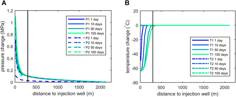
FIGURE 2. (A) Short-term pressure evolution during first 100 days after onset injection; 200 m fracture spacing, (B) short-term temperature evolution during first 100 days after onset injection; 200 m fracture spacing. Solid lines (T1, P1) indicate values in the fractures, dashed lines (T2, P2) in the matrix. The black vertical line represents the horizontal position of the fault, measured at mid-height reservoir level.
Figure 3 presents the long-term evolution of temperatures in the fractures and rock matrix for both the 2 m fracture distance and the 200 m fracture distance. In case of the 2 m fracture distance, the delay in cooling between rock matrix and fractures is very limited, resulting in almost equal mean equilibrium temperatures for fractures and matrix. Consequently, the temperature gradients observed in the rock matrix follow gradients in the fractures, and the temperature propagates through the rock matrix as a sharp front: over a distance of less than 100 m temperature differences of more than 60°C can exist. In case of the 200 m fracture distance, cooling of the rock matrix is more delayed, resulting in a clear temperature difference between fractures and rock matrix, largest in the first years of injection and gradually declining further away.
FIGURE 3. Long-term temperature evolution in the fractures and rock matrix, (A) for fracture distance of 2 m, (B) for fracture distance of 200 m. Solid lines (T1) indicate fracture temperature change, dashed lines (T2) indicate matrix temperature change. The black vertical line represents the horizontal position of the fault, measured at mid-height reservoir level.
In Figure 4A—f, we present the short- and long-term evolution of pressure, temperature and Coulomb stress change on the fault plane. The stress path on the fault varies and depends on the location of monitoring, due to the 3D geometry of the pressure and temperature front and fault. We choose a monitoring position which is located at the center of the fault (see Figure 1 at y = 0), just below mid-height of the reservoir (at depth = −2,375 m). Stress changes at the early stages of injection result from a combination of direct pore pressure, poro- and thermoelastic effects, whilst fault stress changes at later stages are mainly due to propagation of the temperature front.
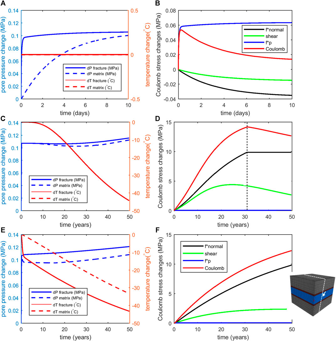
FIGURE 4. Pressure and temperature changes on the fault (central, mid-height location) at 300 m distance from the injection well. (A) pressure and temperature change during first 10 days–fracture distance 200 m, (B) contribution of direct pressure effect (blue), total normal stress changes (black), shear stress (green) to Coulomb stress change on the fault (red), fracture distance 200 m, during first 10 days, (C) pressure and temperature change during total period of 50 years–fracture distance 2 m, (D) contribution of direct pressure effect (blue), total normal stress changes (black), shear stress (green) to Coulomb stress change on the fault (red), fracture distance 2 m, during total period of 50 years. Dashed black line indicates moment normal stresses become tensile. Shear stress declines after 25 years due to the effects of stress arching, (E) pressure and temperature change during total period of 50 years–fracture distance 200 m, (F) contribution of direct pressure effect (blue), total normal stress changes (black), shear stress (green) to Coulomb stress change on the fault (red), fracture distance 200 m, during total period of 50 years.
Figure 4A shows the evolution of pressure and temperature during the first days of injection, for 200 m fracture spacing. Figure 4B presents the associated contributions of pressure, total normal stress and shear stress to the Coulomb stress, and the resulting Coulomb stress change on the fault plane. We use the convention that compressive stress is negative; a positive normal stress change (“unclamping” of the fault) results in an increase of Coulomb stress on the fault. We observe a small, but rapid Coulomb stress loading immediately after the start of the injection operations. This can be explained by the quick diffusion of pressures (P1) in the high permeability fractures, which almost immediately affects the pressures in the fault plane. It is followed by a temporary decrease of Coulomb stresses during the first days, when pressures in the matrix (P2) gradually increase and volumetric changes result in a (stabilizing) poroelastic loading of the fault. Thermo-elastic effects are linked to the temperatures (T2) and thermal strains in the matrix rocks. The role of thermo-elastic stress during the early stages of injection is negligible, as temperature changes in the matrix are still very small. We observe a similar short-term response in our model for the 2 m fracture spacing (not plotted here).
For the long-term temperature effects are dominant. In Figures 4C,E we plot the temperatures and pressures for the 2 m, respectively 200 m fracture spacing. Temperatures in the matrix rocks decrease by −30 to −45°C, whereas pressure changes in both the fractures and the matrix are negligible after the first 100 days.
In both types of reservoirs, cooling and thermal contraction of the matrix rocks leads to a continuous lowering of total normal stresses at the fault which results in “unclamping” of the fault and a positive contribution to the Coulomb stress change (black lines in Figures 4D,F and Eq. 1). The vertical dashed line in Figure 4D shows the level at which effective normal stress at the fault becomes tensile. For the 2 m case we observe tensile stresses at the central monitoring point after 31 years of injection. From that time onwards normal effective stresses are kept constant, as we do not allow opening of the fault. For the 200 m fracture spacing, the normal stress at the fault does not become tensile at this particular location.
As temperatures in the rock matrix decline, fault shear stress in the densely fractured reservoir gradually increases during the first 25 years of injection (Figure 4D). Thereafter shear stresses decline again. The net result are positive Coulomb stress changes, which destabilize this fault location during the first 31 years of injection. The combination of constant normal stress and simultaneous decrease of shear stress during the last 19 years of the injection period results in a net decrease of Coulomb stress (Figure 4D). For the 200 m fracture spacing the shear stress increases during the first 45 years of injection (Figure 4F), whereafter shear stress remains unchanged. In this case Coulomb stress continues to grow up to 50 years (Figure 4F). In both cases the effect of direct pressure on the long-term Coulomb stress changes is negligible.
Figure 5A shows changes in both normal and shear stress with time at a fault position just below mid-height reservoir (at y = 0). The stress paths in Figure 5A can be related to the propagation of the temperature front, which causes arching of stresses within and around the cooling rocks. Thermal compaction of the reservoir causes a decrease of the horizontal stress in the reservoir, both within and around the cooled rock mass. In addition, it causes a decrease of vertical stress within the cooled rock and an increase of vertical stress in the reservoir section just around the cooled area. In Figure 5C we show the change in total vertical stress, for the 2 m fracture spacing. Stress arching affects the shear stress on the fault (see Figure 5C–small graphs). The contribution of shear stress to fault loading varies with position on the fault. Figure 5B shows that after 25 years of injection shear stress on the upper fault segment (above the level of the injection interval), caused by volumetric compaction, add to the shear stress already present from the tectonic loading. The increments in induced shear stresses on the lower fault segment however counteract the in-situ tectonic shear stresses. Effects of stress arching are most pronounced for the 2 m fracture spacing, where a sharp temperature front evolves.
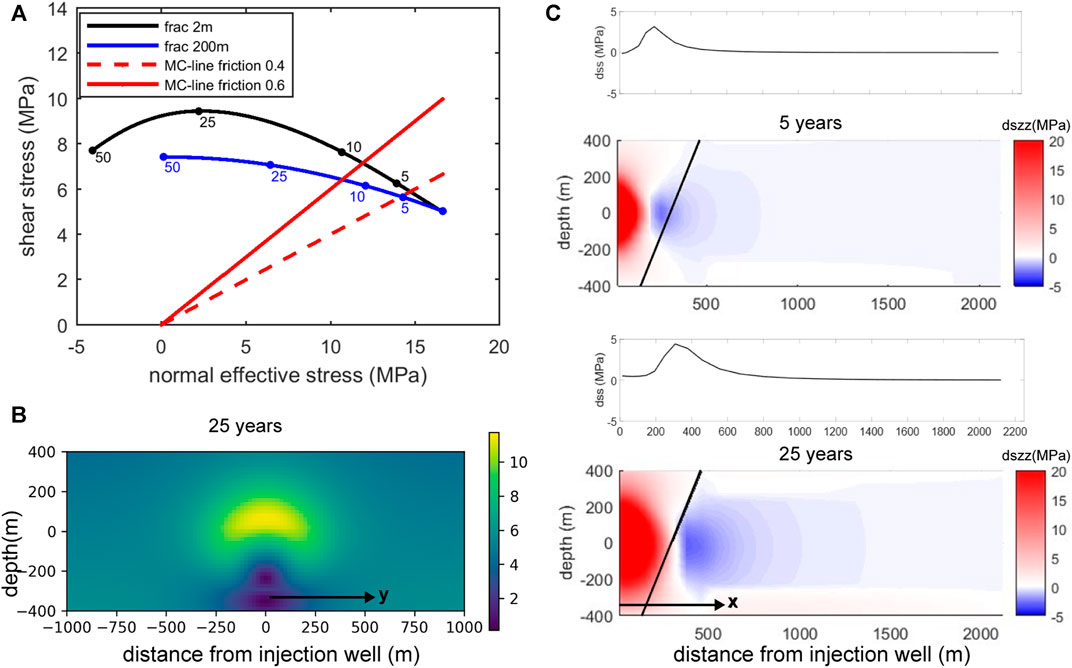
FIGURE 5. (A) Stress path at the fault, just below mid-height reservoir at location y = 0, for both small and large fracture spacing. The four circles on the stress paths indicate stress conditions at 5, 10, 25, and 50 years after onset of injection. (B) Shear stress at the fault plane. Vertical axis: Mid-height reservoir at 0 m, units in depth (m) along dip. Location of projected injection well at y = 0. (C) Arching of total vertical stress around the cooling rock volume, for 2 m fracture spacing. Contour plots represent a vertical cross section (x-direction) through the injection well, perpendicular to the fault plane. Contour plots show change in total vertical stress (dszz) after 5 and 25 years of injection. Mid-height reservoir at 0 m, units in depth (m) along dip. Location of projected injection well at x = 0. Note compressive stress = negative; hence positive value for dszz means total vertical stress decreases. Black solid line shows position of the fault. Small graphs above contour plots show change in shear stress dss, which affects stress path gradients in (A).
Coulomb stress change is less for the 200 m spaced network than for the 2 m spaced network, mainly because the temperature decrease in the bulk rock mass (the matrix) and the related thermo-elastic stress changes are smaller and more gradual. Rates of Coulomb stress changes during this first period are higher for the 2 m spacing (Figure 4D) than for the 200 m spaced fracture network (Figure 4F). This is confirmed by the direction of the stress path for the two cases, as shown in Figure 5A.
From Coulomb stress change vs time shown in Figure 4, Coulomb stress rates are derived, which are converted to seismicity rates through the Dieterich model (Eq. 2). Figure 6 presents the temporal evolution of relative seismicity rates on the fault (i.e. relative to the tectonic background rates) on a section along-dip at position y = 0. Values are shown for one particular realization (input model values are shown in the caption of Figure 6). Variations in stressing and seismicity rates are relatively large for the 2 m fracture distance (Figure 6A), with high seismicity rates at mid-height of the reservoir during the first 25 years of injection (shear stresses increasing, see also Figures 4D, 5A). During late-stage injection seismicity rates at the central part of the reservoir decrease as shear stresses are reducing, and ultimately vanish once tensile normal stresses evolve. Deeper sections of the fault show significant seismic activity at late-stage injection. Note that distance of the fault plane to the injection interval varies with depth due to fault dip orientation. Fault dip orientation also affects the sign of the change in shear stress (as shown in Figure 5B) and thus the seismicity potential with depth.
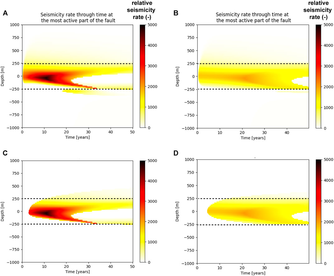
FIGURE 6. Relative seismicity rates versus time after onset of injection for (A) 2 m fracture spacing uncorrected for the size of the perturbed area and (B) 200 m fracture spacing uncorrected for the size of the perturbed area, (C) 2 m fracture spacing, spatial distribution is corrected for the size of the perturbed area and (D) 200 m fracture spacing, spatial distribution is corrected for the size of the perturbed area. Dashed lines indicate top and bottom of reservoir layer. Mid-height reservoir at 0 m, units in depth (m) along dip. Location of projected injection well at y = 0. Relative seismicity rates (R) are shown for one particular realization, with fcrit = 0.4, Mmin = -1, A = 0.001 and
The reservoir with 200 m fracture distance (Figure 6B), characterized by a slower cooling of the reservoir rocks and an absence of a sharp cooling font, shows seismicity rates that are much more constant in time, with the exception of the rapid rise in seismicity rates observed almost immediately after the start of injection. Here relative seismicity rates peak between 20 and 25 years after the onset of injection. Figures 6C,D show relative seismicity rates for the same realization, but now corrected for the size of the critically perturbed area. In both cases, during the first stages of injection no seismicity is expected, as the fault is not yet critically stressed (no perturbed fault area present yet).
Figure 7 shows the evolution of the critically stressed area and the cumulative number of seismic events. We observe that for the 200 m fracture distance, the onset of seismicity is later than for the 2 m fracture distance, due to the slower development of fault criticality. The total critically-perturbed fault area and number of events that nucleate on the entire fault plane is highest for the 2 m fracture distance.
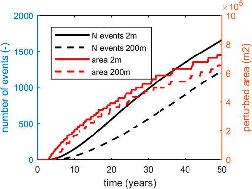
FIGURE 7. Temporal evolution of perturbed area and total number of seismic events for the 2 and 200 m fracture spacing, in a low stress environment.
Figure 8 presents relative seismicity rates at selected times. During the later stages of injection, the spatial pattern of Coulomb stressing rates and relative seismicity rates for the cases with 2 and 200 m fracture spacing is distinctly different. In case of the 2 m fracture distance we observe a clear ring or “halo” of elevated Coulomb stressing and seismicity rates, which is related to higher rates of cooling at the passage of the thermal front (see Figure 8A). Inside, a seismically quiet area arises, where cooling rates after the “passage” of the thermal front have effectively come to an end. Moreover, effective normal stresses within this ring can be tensile. This aseismic area appears at a much later stage for the 200 m fracture distance. The general distribution of seismicity rates for the widely spaced fracture network is more homogeneous.
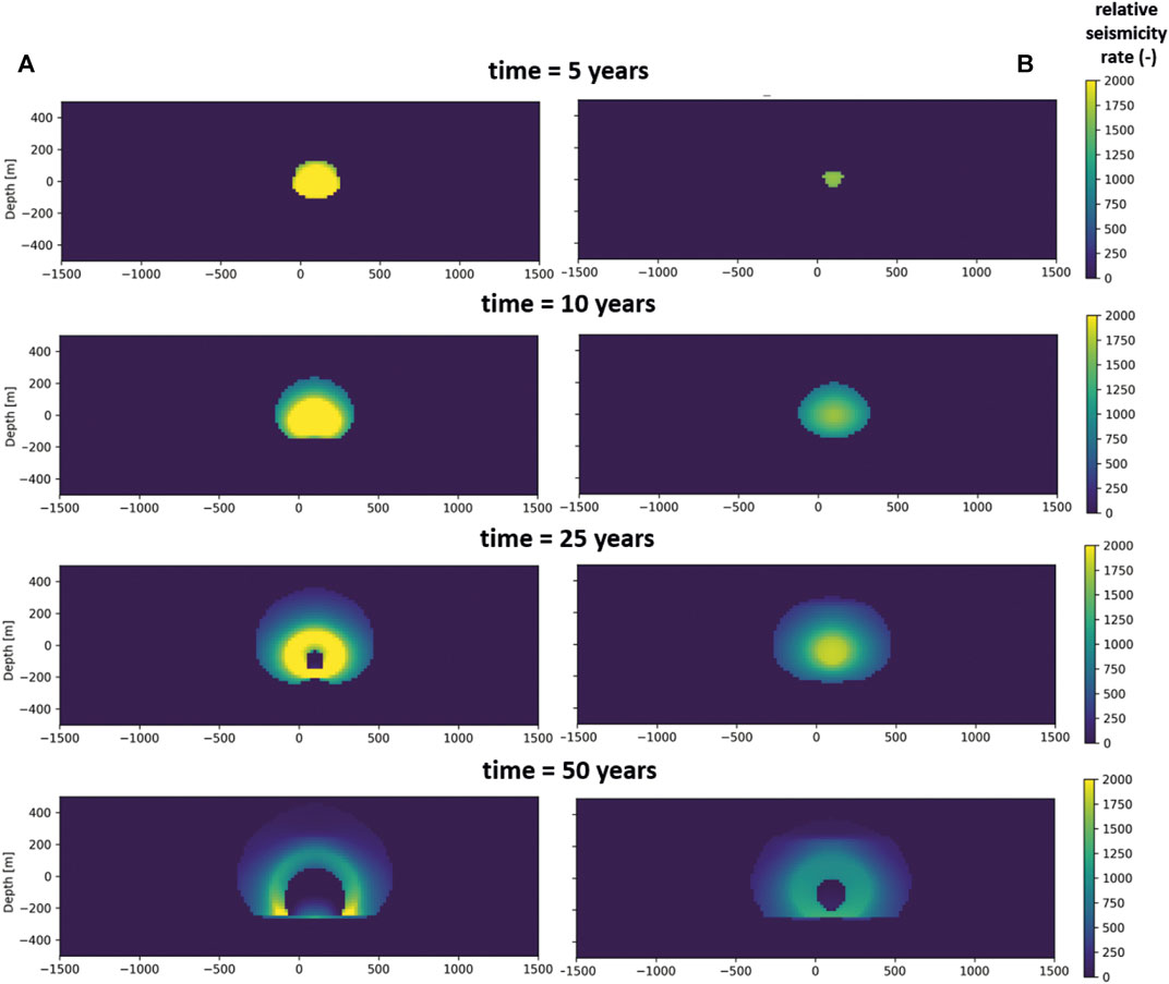
FIGURE 8. Comparison of relative seismicity rates (R) at the fault plane in a low stress environment. Location of projected injection well at y = 0. Left (A) 2 m fracture spacing, right (B) 200 m fracture spacing. Mid-height reservoir at 0 m, units in depth (m) along dip.
Finally, the extent of the perturbed fault area and the seismicity rates are used to derive the temporal evolution of seismicity (as described in Section 2.3). Figure 9A shows an example of the time-dependent truncated Gutenberg-Richter frequency-magnitude distribution of seismic events for the densely fractured carbonate reservoir. The frequency-magnitude distribution shows an increase of the probability of higher magnitudes in time. Note that here we show the outcome for a single realization. The frequency magnitude distribution is created using input parameters and assumptions summarized in Table 2. Figure 9B shows the evolution of cumulative seismic moment release over time in a low stress environment, for both the densely fractured and less damaged carbonate. Cumulative seismic moment release for the 2 m fracture spacing is significantly larger than for the case with 200 m spacing. Rates of seismic moment release for the 200 m fracture spacing during later stages of injection “catch up” with rates of seismic moment release for the 2 m fracture spacing. This is due to the fact that after the passage of the thermal front, a large part of the fault in the densely fractured carbonate reservoir is aseismic. Figure 9C presents estimates of cumulative seismic moment release for the 2 m fractures spacing in a low stress environment, taking into account parameter uncertainty for fault dip, stress drop, threshold fcrit and b-value (parameter ranges used are summarized in Table 2). Estimates for the total amount of seismic moment that is released vary between ∼7 1013 Nm (P10) and 8.7 1014 Nm (P90). However we emphasize that the amount of seismic moment release on the fault is directly dependent on the choice of Mmin. In the current analysis we choose a constant value of Mmin = 0 in combination with a background seismicity rate of r0 = 1 event per year, which means 1 tectonic event occurs per year with a magnitude of at least M = 0. In practice, Mmin and r0 cannot be chosen independently and should be based on the characteristics of the seismic monitoring network (completeness) and the observed natural seismicity rates.
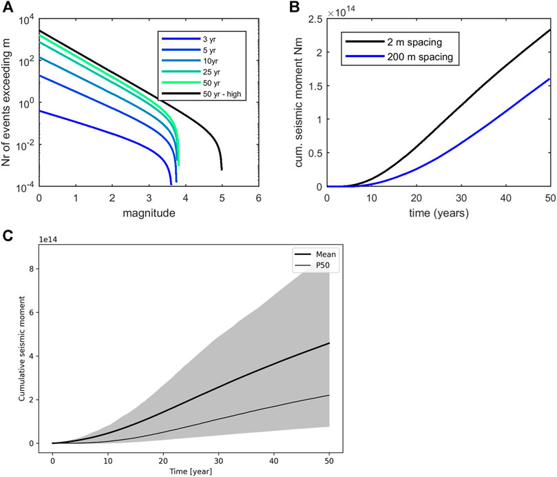
FIGURE 9. (A) Temporal evolution of truncated Gutenberg-Richter frequency-magnitude distribution of seismic events for 2 m fracture distance (single realization). Vertical axis shows number of events
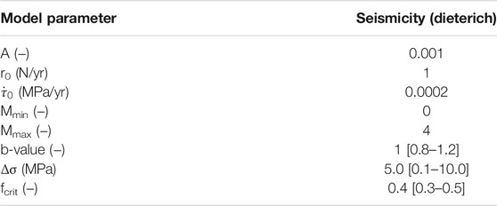
TABLE 2. Parameters and ranges for modelling rate-and-state seismicity and frequency-magnitudes distributions. Values between square brackets indicate a stochastic range of input parameters (uniform distribution).
In current state-of-the-art, fault stability and seismicity potential is mostly assessed based on analysis of Coulomb stress changes and reactivated fault area. In our workflow, we adopt rate-and-state seismicity theory to assess changes in seismicity rates based on Coulomb stressing rates (Segall and Lu, 2015; Maurer and Segall, 2018) in our numerical scheme. We compare the seismic response of a fault during constant-rate injection in a highly fractured and a sparsely fractured carbonate reservoir. Our study indicates that even though the thermal loading is generally slow, stressing rates can still cause elevated seismicity rates during the approach and “passage” of the thermal front through the fault plane. Our models show that stressing rates and seismicity rates in densely fractured carbonates are highest, which can be explained by the propagation of a steep thermal front related to stronger and more localized cooling of the reservoir. This steep thermal front and localized strong cooling promotes arching of stresses and locally and temporarily high Coulomb stressing and seismicity rates. The occurrence of steep thermal fronts are not necessarily limited to densely fractured carbonates. Steep temperature gradients can also occur in more homogeneous porous sandstone reservoirs, specifically under low injection rates.
The effects of varying thermal loading rates in time and space on fault stability and seismic risk need to be further understood to enable long-term seismic risk assessment of injection operations. We note that we compare the “seismic footprint” in the densely fractured and less damaged carbonates under the assumption that the rate-and-state parameters for the fault in both types of reservoirs are similar. In reality, rate-and-state parameters for faults in different types of carbonate reservoirs may differ.
Another point of attention is the change of nucleation length (the minimum length of critically stressed fault required for seismic rupture to occur) during progressive cooling of the reservoir. As shown, the simultaneous increase of pressures and thermal contraction of the rocks during injection may lead to very low effective normal stresses on the fault plane. The nucleation length tends to increase with lowering normal effective stress. Also, in the current study stress drop was assumed constant, but in reality the stress drop will decrease as the normal stress decreases as they are linked through frictional weakening. This would lead to smaller events or even aseismic behavior. It needs to be further analyzed in what way low normal stresses influence the role of aseismic fault slip during progressive cooling of the rocks.
The dimensions of the fault segment that becomes critically stressed during operations form an important factor for the magnitude of seismic events in a low stress environment. At present, our method is based on the assumption that the rupture area of the seismic events is circular. More insight is needed on what aspect ratios of fault rupture can realistically occur in elongated reservoirs that are potential targets for geothermal energy production, and what is the effect of reservoir confinement on frequency-magnitude distributions and seismic risks.
In our approach we aim to analyze the loading of a fault by the pressure and temperature changes in the surrounding medium. In our simplified model, we do not account for the presence of damage zones around faults with locally high fracture density, nor the effects of fault barriers and sealing faults. Anisotropies caused by the presence of high permeability flow paths in damage zones or low permeability fault cores impeding fault-perpendicular flow will affect the pressure and temperature fields, fault loading and seismicity (Wassing et al., 2021).
The workflow has been demonstrated for a synthetic injection case in a fractured carbonate reservoir. Seismicity is dependent on a large number of input parameters, most of which are poorly constrained before the start of the operations. As shown in Figure 9, parameter uncertainty has a large effect on the estimates of seismic moment release. As a result, at this stage the workflow can only be used for a relative “ranking” of reservoirs of different characteristics. Input data for models are generally poorly constrained, therefore models need to be calibrated and validated based on data from seismic monitoring networks. Parameter ranges and uncertainties need to be constrained based on information from (seismicity) monitoring: details on the specifics of the network used for seismic monitoring (e.g. level of completeness defining Mmin), mapped total fault area and fault density, stress drops, seismicity rates and magnitudes recorded during the injection operations. In addition to monitoring during operations, the understanding of changes in seismicity rates and seismicity potential of the faults requires monitoring of background seismicity rates well in advance of the injection operations. A closed loop of seismic monitoring (near-)real-time data-assimilation and model updating is considered crucial for a robust estimation and update of seismic risks during injection operations.
We built a workflow to assess the evolution of seismicity associated to injection of cold fluids in a single injector close to a fault. We employ the coupled numerical thermo-hydro-mechanical simulator of FLAC3D-TOUGHREACT to simulate the spatial and temporal evolution of pore pressures and temperatures in a fractured carbonate reservoir and the associated Coulomb stress changes on the fault. Adopting rate-and-state seismicity theory we assess induced seismicity rates from Coulomb stressing rates at the fault. Seismicity rates are then used to assess the evolution of seismicity in terms of the time-dependent frequency-magnitude distribution of seismic events. We compare the seismic response of a fault in a highly fractured and a sparsely fractured carbonate reservoir. We analyze the effect of tectonic regime and compare the seismic response in a low-stress and high-stress environment. From the above analysis, we draw the following conclusions:
• The seismic response of the fault, in terms of the timing of the peaks of elevated seismicity and total seismic moment release, depends on the fracture density, because this density affects the heat exchange rate between cold fluid in the fractures and the intermediate matrix and hence the temperature decrease in the bulk rock volume and thermo-elastic stress change.
• A dense fracture network results in a steeper thermal front which promotes stress arching, which leads to locally and temporarily high Coulomb stressing rates. The total seismic moment release is consequently largest for the densely spaced fracture network. Also, it occurs at an earlier stage of the injection period: the release is more gradually spread in time and space for the widely spaced fracture network.
• Frequency-magnitude distributions and seismic moment release have been derived both for a low-stress subsurface and a tectonically active area with initially critically stressed faults. The evolution of seismicity in the low-stress environment depends on the dimensions of the fault area that is perturbed by the induced stress changes. The probability of larger, “felt”, earthquakes and the associated seismic risk are thus reduced in low-stress environments.
• Injection of cold fluids into a competent rock like carbonate causes cooling of the reservoir and significant thermal stresses. Pore pressures reach steady-state conditions relatively quickly, but the evolution of seismicity during injection over the long-term is non-stationary: we observe an ongoing increase of the fault area that is critically stressed as the cooling front continues to propagate from the injection well into the reservoir. During later stages, models show the development of an aseismic area surrounded by an expanding ring of high Coulomb stressing and seismicity rates at the edge of the cooling zone. This ring can be related to the “passage” of the cooling front.
• Input data are generally poorly constrained, therefore models need to be calibrated and validated based on data from seismic monitoring networks. A closed loop of seismic monitoring (near-)real-time data-assimilation and model updating is considered crucial for a robust estimation and update of seismic risks during injection operations.
The original contributions presented in the study are included in the article/Supplementary Material, further inquiries can be directed to the corresponding author.
BW, TC, and SO contributed to conception and design of the study. BW, TC, EP, and SO performed the modelling and interpretation of results, BW, TC, LB, PF, and JW wrote sections of the manuscript. All authors contributed to manuscript revision, read, and approved the submitted version.
This project has been subsidized through the ERANET Cofund GEOTHERMICA (Project no. 731117), from the European Commission, Topsector Energy subsidy from the Ministry of Economic Affairs of the Netherlands, Federal Ministry for Economic Affairs and Energy of Germany and EUDP. The workflow was partially developed using funding from the European Union’s Horizon 2020 research and innovation programme under grant agreement number 764531, project SECURe.
The authors declare that the research was conducted in the absence of any commercial or financial relationships that could be construed as a potential conflict of interest.
All claims expressed in this article are solely those of the authors and do not necessarily represent those of their affiliated organizations, or those of the publisher, the editors and the reviewers. Any product that may be evaluated in this article, or claim that may be made by its manufacturer, is not guaranteed or endorsed by the publisher.
Baisch, S., and Vörös, R. (2018). Earthquakes Near the Californie Geothermal Site: August 2015 – November 2018. Prepared for Californie Lipzig Gielen Geothermie BVReport No. CLGG005. Q-con GmbH.
Bouroullec, R., Nelskamp, S., Kloppenburg, A., Abdul Fattah, R., Foeken, J., Ten Veen, J., et al. (2019). Burial and Structural Analysis of the Dinantian Carbonates in the Dutch Subsurface. Report by SCAN. scan_dinantian_burial_and_structuration_report.pdf .
Buijze, L., van Bijsterveldt, L., Cremer, H., Paap, B., Veldkamp, H., Wassing, B. B., et al. (2019). Review of Induced Seismicity in Geothermal Systems Worldwide and Implications for Geothermal Systems in the Netherlands. Neth. J. Geosciences 98. doi:10.1017/njg.2019.6
Candela, T., Van Der Veer, E. F., and Fokker, P. A. (2018). On the importance of thermo-elastic stressing in injection-induced earthquakes. Rock Mech. Rock Eng. 51 (12), 3925–3936.
Candela, T., Osinga, S., Ampuero, J. P., Wassing, B., Pluymaekers, M., Fokker, P. A., et al. (2019). Depletion‐Induced Seismicity at the Groningen Gas Field: Coulomb Rate‐and‐State Models Including Differential Compaction Effect. J. Geophys. Res. Solid Earth 124 (7), 7081–7104. doi:10.1029/2018JB016670.2019
Chen, J., Donald, J., and Huang, H., (2013). Determination of thermal Conductivity of Carbonate Cores. SPE 165460. doi:10.2118/165460-ms
Dieterich, J. (1994). A Constitutive Law for Rate of Earthquake Production and its Application to Earthquake Clustering. J. Geophys. Res. 99, 2601–2618. doi:10.1029/93jb02581
Gan, Q., and Elsworth, D. (2014). Thermal Drawdown and Late‐stage Seismic‐slip Fault Reactivation in Enhanced Geothermal Reservoirs. J. Geophys. Res. Solid Earth 119, 8936–8949. doi:10.1002/2014jb011323
Heimisson, E. R., and Segall, P. (2018). Constitutive Law for Earthquake Production Based on Rate‐and‐State Friction: Dieterich 1994 Revisited. J. Geophys. Res. Solid Earth 123, 4141–4156. doi:10.1029/2018JB015656
IEA (2020). Geothermal. Paris: IEA. available at: https://www.iea.org/reports/geothermal.
Jacquey, A. B., Cacace, M., Blöcher, G., and Scheck-Wenderoth, M. (2015). Numerical Investigation of Thermoelastic Effects on Fault Slip Tendency during Injection and Production of Geothermal Fluids. Energ. Proced. 76, 311–320. doi:10.1016/j.egypro.2015.07.868
Lipsey, L., Pluymaekers, M., Goldberg, T., Van Oversteeg, K., Ghazaryan, L., Cloetingh, S., et al. (2016). Numerical Modelling of thermal Convection in the Luttelgeest Carbonate Platform, the Netherlands. Geothermics 64, 135–151. doi:10.1016/j.geothermics.2016.05.002
Maurer, J., and Segall, P. (2018). Magnitudes of Induced Earthquakes in Low‐Stress Environments. Bull. Seismological Soc. America 108 (3A), 1087–1106. doi:10.1785/0120170295
Rubin, A. M., and Ampuero, J.-P. (2007). Aftershock Asymmetry on a Bimaterial Interface. J. Geophys. Res. 112, BO5307. doi:10.1029/2006JB004337
Segall, P., and Lu, S. (2015). Injection-induced Seismicity: Poroelastic and Earthquake Nucleation Effects. J. Geophys. Res. Solid Earth 120, 5082–5103. doi:10.1002/2015jb012060
State Supervision of Mines, (2019). Analyse onderbouwing CLG aardwarmte en seismiciteit. The Hague: Technical Report , Staatstoezicht op de Mijnen (State Supervision of Mines).
Taron, J., and Elsworth, D. (2010). Coupled Mechanical and Chemical Processes in Engineered Geothermal Reservoirs with Dynamic Permeability. Int. J. Rock Mech. Mining Sci. 47, 1339–1348. doi:10.1016/j.ijrmms.2010.08.021
Ter Heege, J., van BijsterveldtWassing, L. B., Osinga, S., Paap, B., and Kraaijpoel, D. (2020). Induced Seismicicity Potential for Geothermal Projects Targeting Dinantian Carbonates in the Netherlands. Utrecht: Final report by SCAN.
Van Wees, J-D., Kahrobaei, S., Osinga, S., Wassing, B., Buijze, L., Candela, T., et al. (2019a). 3D Models for Stress Changes and Seismic hazard Assessment in Geothermal Doublet Systems in the Netherlands. Reykjavik, Iceland: World Geothermal Congress 2020. April 26-May 2, 2020; submitted.
Van Wees, J. D., Veldkamp, H., Brunner, L., Vrijlandt, M., De Jong, S., Heijnen, N., et al. (2020). Accelerating Geothermal Development with a Play-Based Portfolio Approach. Neth. J. Geosciences 99. doi:10.1017/njg.2020.4
Vöros, R., and Baisch, S. (2019). Seismic hazard Assessment for the CLG-Geothermal System – Study Update March 2019, Report No. CLG006. Q-con GmbH.
Wassing, B. B. T., Van Wees, J. D., and Fokker, P. A. (2014). Coupled continuum modeling of fracture reactivation and induced seismicity during enhanced geothermal operations. Geothermics 52, 153–164.
Keywords: injection-induced seismicity, geothermal operations, seismic hazard, long-term thermal loading, fractured carbonates
Citation: Wassing BBT, Candela T, Osinga S, Peters E, Buijze L, Fokker PA and Van Wees JD (2021) Time-dependent Seismic Footprint of Thermal Loading for Geothermal Activities in Fractured Carbonate Reservoirs. Front. Earth Sci. 9:685841. doi: 10.3389/feart.2021.685841
Received: 25 March 2021; Accepted: 24 August 2021;
Published: 14 September 2021.
Edited by:
Antonio Pio Rinaldi, Swiss Seismological Service, ETH Zurich, SwitzerlandReviewed by:
Zahid Rafi, Pakistan Meteorological Department, PakistanCopyright © 2021 Wassing, Candela, Osinga, Peters, Buijze, Fokker and Van Wees. This is an open-access article distributed under the terms of the Creative Commons Attribution License (CC BY). The use, distribution or reproduction in other forums is permitted, provided the original author(s) and the copyright owner(s) are credited and that the original publication in this journal is cited, in accordance with accepted academic practice. No use, distribution or reproduction is permitted which does not comply with these terms.
*Correspondence: B. B. T. Wassing, YnJlY2h0Lndhc3NpbmdAdG5vLm5s
Disclaimer: All claims expressed in this article are solely those of the authors and do not necessarily represent those of their affiliated organizations, or those of the publisher, the editors and the reviewers. Any product that may be evaluated in this article or claim that may be made by its manufacturer is not guaranteed or endorsed by the publisher.
Research integrity at Frontiers
Learn more about the work of our research integrity team to safeguard the quality of each article we publish.