Research on Deep Convolutional Neural Network Time-Frequency Domain Seismic Signal Denoising Combined With Residual Dense Blocks

Deep Convolutional Neural Networks (DCNN) have the ability to learn complex features and are thus widely used in the field of seismic signal denoising with low signal-to-noise ratio (SNR). However, the current convolutional deep network used for seismic signal noise reduction does not make full use of the feature information extracted from all convolution layers in the network, and thus cannot fit the seismic signal with high SNR. To deal with this problem, this paper proposes the DnRDB model, a convolutional deep network time-frequency domain seismic signal denoising model combined with residual dense blocks (RDB). The model is mainly composed of several RDB in series. The input of each convolution layer in each RDB module is formed by the output of all the previous convolution layers. Meanwhile, even if the number of layers is increased, the fusion of the seismic signal features learned by the RDB modules can still achieve full extraction of seismic signals. Furthermore, deepening the model structure by concatenating multiple RDB modules enables further useful feature information to be extracted, which improves the SNR of seismic signals. The DnRDB model was trained and tested using the Stanford Global Seismic Dataset. The experimental results show that the DnRDB model can effectively recover seismic signals and remove various forms of noise. Even in the case of high noise, the denoised signal still has a high SNR. When the DnRDB model is compared with other denoising approaches such as wavelet threshold, empirical mode decomposition, and different deep learning methods, the results indicate that it performs best overall in denoising the same segment of the noisy seismic signal; the denoised signal also has less waveform distortion. Use of the DnRDB model in subsequent seismic signal processing work indicates that it can help the phase recognition algorithm improve the accuracy of seismic recognition through noise reduction.

Introduction

In most cases, big earthquakes cause a large number of casualties and extensive property loss. An early warning system can be an effective measure to reduce disasters. Accurate seismic data can help such systems obtain accurate arrival time, but their accuracy is usually strongly affected by the impact of different kinds of noise (Zhang et al., 2019). As a result, methods of seismic signal denoising have been extensively studied by researchers at home and abroad.

Traditional seismic signal denoising methods mainly include Fourier transform (Ming-Yue, and Zhai, 2014; Zhang and Cai, 2014), wavelet transform (Cao and Chen, 2005; Gaci and Said, 2014; Mousavi et al., 2016), empirical mode decomposition (EMD) (Huang et al., 1998; Bekara and Baan, 2011; Chen and Ma, 2014; Han and Mirko, 2015) and so on. The Fourier transform removes noise by transforming the signal from the time to the frequency domain, analyzing the difference between the frequency range of the noise and the clean seismic signal. However, a Fourier transform cannot display time and frequency information at the same time, it can obtain the global spectrum of the signal instead of the local characteristic. This means the local characteristics of nonstationary seismic signals cannot be identified. Wavelet transform can reduce noise by virtue of mapping a one-dimensional time domain signal to a two-dimensional time-frequency domain so that it can also handle nonstationary seismic signals, but this is highly threshold dependent and the basis function needs to be selected according to the actual signal. EMD uses the timescale characteristics of the signal itself to decompose it without using any basis function. It forms a part of the Hilbert Huang transform proposed by Huang and others in 1998 (Huang et al., 1998), and is also a self-adaptive signal analysis method. The nonlinear, nonstationary signal is decomposed into a natural mode function that satisfies the Hilbert transform, then the natural mode function of noise is removed so as to obtain the denoising signal. Although EMD can remove noise to a certain extent, it also has some problems, such as mode aliasing and difficulty in selecting an eigenfunction. The denoising results are strongly affected by the manually selected eigenfunctions or threshold parameters, which limit performance. This is particularly true under the condition of low signal-to-noise ratio (SNR). Despite these limitations, traditional denoising methods have greatly improved the quality of seismic data.

Since AlexNet won the ILSVRC (ImageNet Large-Scale Visual Recognition on Challenge) in 2012 (Krizhevsky et al., 2012), the deep neural network method has been widely applied to image recognition (Ronneberger et al., 2015; Zhang et al., 2020), image denoising (Mao et al., 2016; Zhang et al., 2016), speech processing (Huang et al., 2014; Weninger et al., 2014; Huang et al., 2015) and other fields because of its strong feature learning and nonlinear mapping abilities. It also has the advantages of requiring no manual participation and having low computing costs. Therefore, a large number of scholars have begun to try to apply deep neural networks to seismic signal denoising (Jin et al., 2018; Yu et al., 2018; Dong et al., 2020). In 2018, Yu et al. (2018) used a multilayer convolutional neural network to perform the self-adaptive denoising of seismic signals containing different kinds of noise. The experimental results showed that the denoising effect of this algorithm outperformed the traditional algorithm while the denoising effect is limited by the number of layers in the network. If there are fewer network layers, fewer signal features can be learned, resulting in a low SNR. However, increasing the number of network layers will lead to gradient disappearance and other problems. In the same year, Jin et al. (2018) used a new autoencoder based on a deep residual network to achieve the random noise reduction of seismic signals. Their algorithm combined a convolutional autoencoder with the residual network to avoid the problem of gradient disappearance found in the deep network. However, it is noticeable that a seismic signal is a typical nonstationary signal, and its frequency distribution is not fixed. When the frequency of the seismic signal is confused with that of noise (i.e., they are the same), a general deep neural network cannot completely separate signal from noise. This means that the denoised signal actually contains more noise, and the SNR remains low. In 2019, Zhu et al. (2019) studied a seismic signal denoising method in a time-frequency domain based on a U-Net called DeepDenoiser. According to the characteristics of how the contraction path is used to improve the sparseness of the input signal and the extended path is used to extract the clean signal, some features of the contraction path can be reused by means of the jump connection. As a result, it can retain more features of the seismic signal and improve the convergence speed of model training. In addition, even when the signal and noise frequencies are confused, the latter can be effectively suppressed. Nevertheless, the U-Net does not make full use of the output characteristics of each convolutional layer in the network, and thus cannot fully extract the features of the seismic signal, resulting in an unsatisfactory improvement of the SNR of the seismic signal.

In 2018, Zhang et al. (2018) proposed a residual dense block (RDB) that can fully extract features from images. The RDB module mainly contains a dense connection layer and feature fusion with residual learning. The dense connection structure can widen the network and strengthen the reuse of feature information. Feature fusion with residual learning can combine the extracted feature information of all convolutional layers in the current module with the output information of the previous module, and the fused feature map makes full use of the feature information extracted from each convolutional layer in the module. In 2019, Kim et al. (2019) used Grouped Residual Dense Network (GRDN) for real image denoising. The experimental results showed that the GRDN network significantly improves the image denoising performance by fully extracting image features with the RDB modules. In 2020, Li et al. (2020) used the RDB modules as the basic module of a residual dense network for hyperspectral reconstruction. Their experimental results proved that the RDB modules improved accuracy. These studies indicate that RDB modules are superior in terms of image feature extraction and can improve the SNR of an image.

In summary, in order to improve the SNR of complex seismic signals, this paper proposes a convolutional deep network time-frequency domain seismic signal denoising model combined with a RDB (DnRDB). The model is mainly composed of multiple RDBs connected in series. The RDB module is able to fully extract the characteristics of the time-frequency domain seismic signals through the fusion of a dense connection structure and features with residual learning. Experiments with training and testing of original data recorded by seismic stations emphasize that the DnRDB model can effectively restore seismic signals and remove various types of noise. Even in high-noise situations, the denoising signal still has a high SNR. In comparison with wavelet transform, EMD noise reduction, and other deep learning algorithms, DnRDB has better denoising performance and can improve the accuracy of a seismic phase recognition algorithm accordingly.

Denoising Model Combined With a Residual Dense Blocks Denoising Model

As time-frequency domain signals can simultaneously express information about both the signal time and frequency domains, converting nonstationary seismic signals from the time domain to the time-frequency domain is more conducive to the model being able to learn their features. This is why the DnRDB model processes data in the time-frequency domain.

In the time-frequency domain, noisy seismic signals containing various noises can be expressed as:

$\begin{array}{c}Y\left(\mathit{t},\mathit{f}\right)=X\left(\mathit{t},\mathit{f}\right)+N\left(\mathit{t},\mathit{f}\right)\end{array}(1)$

Here, $Y\left(t,f\right)$ represents the noise-containing seismic signal recorded by seismic stations, $X\left(t,f\right)$ represents a clean seismic signal, and $N\left(t,f\right)$ represents all kinds of noise contained in the recorded data of seismic stations. The noisy seismic signal $Y\left(t,f\right)$ can be regarded as the superposition of the clean seismic signal $X\left(t,f\right)$ and the noise $N\left(t,f\right)$. The purpose of noise reduction is to remove various noises from seismic signals and clean them as accurately as possible.

DnRDB is a supervised network which takes the seismic signal containing noise in the time-frequency domain as input and the time-frequency mask as the output target. The predicted time-frequency mask, in the time-frequency domain, can effectively retain seismic signal components and suppress noise components, so as to achieve the purpose of noise reduction. The work reported in this paper utilizes the amplitude-time-frequency mask commonly used in speech noise reduction (Huang et al., 2015), whose formula is as follows:

$\begin{array}{c}M\left(\mathit{t},\mathit{f}\right)=\frac{\left|\mathit{X}\left(\mathit{t},\mathit{f}\right)\right|}{\left|\mathit{X}\left(\mathit{t},\mathit{f}\right)\right|+\left|\mathit{N}\left(\mathit{t},\mathit{f}\right)\right|}\end{array}(2)$

The size of each mask is the same as the input of the time-frequency domain seismic signal $Y\left(t,f\right)$, and the value is between 0–1, indicating the proportion of clean seismic signal within the noisy seismic signal. A well-trained model can predict the time-frequency mask $\widehat{M}\left(t,f\right)$ and the seismic signals in the time-frequency domain after denoising can be calculated from the seismic signals containing noise. The formula is as follows:

$\begin{array}{c}\widehat{\mathit{X}}\left(\mathit{t},\mathit{f}\right)=\widehat{\mathit{M}}\left(\mathit{t},\mathit{f}\right)Y\left(\mathit{t},\mathit{f}\right)\end{array}(3)$

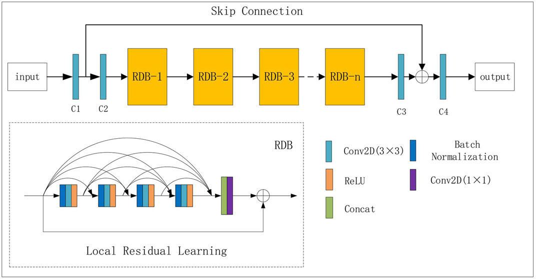
The structure of the DnRDB is composed of input, middle, and output layers. The specific model structure is shown in (Figure 1).

FIGURE 1

FIGURE 1. The DnRDB model structure.

The input layer is composed of two convolutional layers, the first of which is used to read the input time-frequency domain noisy seismic signal $Y\left(t,f\right)$, and the second aims to further extract the signal features as the input of the middle layer. The feature map of each convolutional layer is set as 32, the size of the convolution kernel as 3 × 3, and the convolution step size as 1.

The middle layer is a series of multiple RDBs which mainly adopt dense connection layers and the local feature fusion with the local residual learning functions to fully extract the features of the seismic signals. In each RDB module, the dense connection layer connects all the other layers in a feed-forward manner. In terms of each layer, the feature maps of all previous layers are used as the input, and its own feature maps provide the input for all subsequent layers (Huang et al., 2016). The dense connection merges the information from all layers as much as possible to form a continuous memory mechanism and distribute the information that needs to be retained. In addition to making up the convolutional layer and the activation function ReLU [max (0,y)] (Nair and Hinton, 2010), Batch Normalization (BN) (Ioffe and Szegedy, 2015) is added after the convolution layer to ensure the input of each layer has a stable distribution. As a consequence, the generalization ability and convergence speed of the denoising network can be improved while the gradient dispersion is avoided effectively. Feature fusion with residual learning performs the merging between the output information of the previous RDB module and the information from all the convolutional layers of the current RDB module. The convolution layer whose kernel is 1 × 1 is used to sort the feature image information, and the information after feature fusion is added to the output information of the previous RDB module. This can improve the information flow and allow a larger number of features, which helps to improve model performance. The number of convolutional layers of each RDB module in the middle layer is 4, the number of feature maps of each convolutional layer is 32; the size of the convolution kernel is set as 3 × 3, and the convolution step size is set as 1.

The output layer is also composed of two convolutional layers. The first is used to read the signal features output by the middle layer, and the last outputs the results predicted by the model. Using skip connections between the input and output layers makes the model output retain more effective seismic signal features and enhances the transmission of gradient information. The feature map of the first layer is set as 32, and the number of the feature map of the last layer is 1; that is, the time-frequency mask of the predicted clean signal. The size of the convolution kernel of the output layer is set as 3 × 3, and the convolution step size as 1.

During training, the network obtains the predicted time-frequency mask by learning the input time-frequency domain seismic signals. It then uses Eq. (2) to calculate the time-frequency mask as the final optimization target value of the network (the network training label). The loss function is then applied to measure the distance between the predicted and desired target values by repeatedly comparing the difference between the two and constantly adjusting the hyperparameters of the network to minimize this. The loss function used by DnRDB is the mean square error loss. The specific formula is as follows:

$\begin{array}{c}l=\frac{1}{2\mathit{N}}{\displaystyle \sum _{\mathit{i}=1}^{\mathit{N}}{\Vert \widehat{\mathit{M}}\left(\mathit{t},\mathit{f}\right)-\mathit{M}\left(\mathit{t},\mathit{f}\right)\Vert }_F^2}\end{array}(4)$

In the formula, ‖∙‖ represents the Frobenius norm, $M\left(t,f\right)$ is the label for network training, and $\widehat{M}\left(t,f\right)$ is the output of the DnRDB model; that is, the predicted time-frequency mask.

The denoising process of seismic signals by DnRDB model completed by training is as follows. Firstly, the noisy seismic signal in time domain is transformed into the time-frequency domain. Secondly, the noisy seismic signals $Y\left(t,f\right)$ so converted are input into the model. After the calculation of all layers of the model, the predicted time-frequency mask $\widehat{M}(t,f)$ is output. Then, according to Eq. 4, the noisy seismic signal Y (t,f) and the output mask $\widehat{M}\left(t,f\right)$ are used to calculate the predicted denoised time-frequency domain signal $\widehat{X}\left(t,f\right)$. Finally, an inverse short-time Fourier transform is performed on X ̂(t,f) to obtain the final denoised time-domain seismic signal.

Experiment and Analysis

Determination of the Number of Residual Dense Blocks Modules

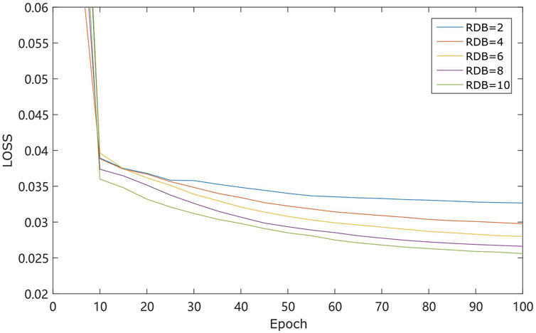
In the DnRDB model, the increase of the number of RDB modules also increases the depth of the network, which theoretically helps to improve performance. However, at the same time, it also consumes a lot of video memory, resulting in increased training time. We therefore need to comprehensively consider the appropriate number of RDB modules required to determine the training time and the mean square error loss. In our experiment, a dataset containing 600 seismic waveforms was applied to test these variables under the five conditions of 2, 4, 6, 8, and 10 RDB modules, respectively, so as to identify the optimal number. The number of convolution layers of each RDB is 4, the number of convolution layer feature maps is 32, the convolution core size is set as 3 × 3, and the convolution step size is set as 1. The experimental results are shown in (Figure 2). This presents the mean square error loss of the different numbers of RDB modules, all trained 100 epoch. As can be seen from the experimental results, an increase in the number of RDB modules results in a gradual decrease in the mean square error loss after the completion of training. The number of RDB modules is proportional to the training effect; however, the network training time increases linearly with the increase in RDB modules, and the epoch times are 3, 6, 9, 12, and 15 s respectively. To sum up, the selection of 8 RDB modules is appropriate under the conditions of considering the time cost and ensuring the reduction of the mean square error loss.

FIGURE 2

FIGURE 2. The mean square error loss curves.

Denoising Model Combined With a Residual Dense Blocks Model Training and Test Analysis

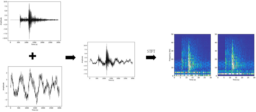
The sample data used in the experiment comes from the Stanford Earthquake Dataset (STEAD) published by Stanford University, which is the world’s first globally labeled dataset of high-quality seismic and nonseismic signals recorded by seismic instruments (Mousavi et al., 2019). Network training and testing require noisy seismic signals. In this paper, those are synthesized by combining clean seismic signals with noise. However, clean seismic signals cannot be obtained in seismic data acquisition, so 82,380 seismic event signals with high SNR in STEAD were selected as the clean sample in this dataset. A total of 199,760 nonseismic signals in STEAD were selected as noise samples and randomly combined with the clean signal samples to obtain a large sample set of noisy seismic signals. Firstly, each clean seismic signal sample was randomly shifted. Secondly, a noise sample was randomly selected and its amplitude scaled at random, superimposing it on the clean seismic signal sample to generate noisy seismic signals with different SNR levels. Finally, in order to achieve the purpose of accelerating the convergence speed during network training, the noisy signals were normalized by subtracting the mean value and dividing by the standard deviation. All the signals in the dataset were uniformly cut to a length of 30 s (longer signals were cut from the tail) because in the selected set of high-SNR signals, the first 30 s basically includes the main waveform of the event. As all training and testing of the algorithm in this paper was performed in the two-dimensional time-frequency domain, it was necessary to convert the one-dimensional time-domain seismic signal. The short-time Fourier transform method was adopted for conversion, and the basic formula is as follows:

$\begin{array}{c}\mathit{STF}{\mathit{T}}_{\mathit{x}}\left(\mathit{t},\mathit{f}\right)={\displaystyle \sum }_{\mathit{n}=0}^{\mathit{L}-1}\mathit{x}\left(\mathit{n}\right)\mathit{m}\left(\mathit{n}-\mathit{t}\right){\mathit{e}}^{-\mathit{j}2\mathit{\pi fn}}\end{array}(5)$

Here, $x\left(n\right)$ represents the original signal at time n, $m\left(n\right)$ represents the sliding window function of the original signal at time n, and L represents the length of the window function. t represents the time in the time-frequency domain, f represents the frequency in the time-frequency domain. After conversion, the two-dimensional time-frequency domain matrix of the seismic signal obtained is 31 × 201. The pipeline from raw data to the input of the network is shown in Figure 3.

FIGURE 3

FIGURE 3. The pipeline from raw data to the input of the network.

The dataset was randomly divided into training, validation, and testing set in a ratio of 80, 10 and 10%. The training set was used to train the model, the validation set is only used for tuning the hyper-parameters of the network and the test set to evaluate the noise reduction effect.

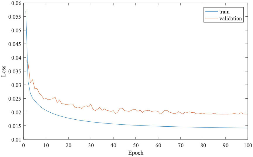
During the training, the noisy seismic signal transformed from the training set to the time-frequency domain is used as the input of the network, and the time-frequency mask calculated by Eq. 2 is used as the label. In the experiment, TensorFlow was used to build the model, and the training set was adopted to train on the Graphics Processing Unit. It is necessary to set the initial learning rate for training as 0.001, use the Adam optimization algorithm to optimize the learning objectives, set the epoch as 100 times, and set the batch size as 16. After approximately 37 h of training, a trained model was obtained. Figure 4 shows the loss reduction curve of the training set and the validation set. In the figure, the model training loss and the validation loss still keep decreasing at 100 epoch, indicating that the model has not been overfitted.

FIGURE 4

FIGURE 4. Training loss and validation loss declining curve.

In this paper, two indicators, SNR and the correlation coefficient ($r(X,Y)$), are used to quantitatively evaluate the effect of noise reduction. The formulae for each are as follows:

$\begin{array}{c}SNR=10{\log }_{10}\left(\frac{{\mathit{\sigma }}_{\mathit{s}}}{{\mathit{\sigma }}_{\mathit{n}}}\right)\end{array}(6)$

$\begin{array}{c}r(X,Y)=\frac{\mathit{Cov}\left(\mathit{X},\mathit{Y}\right)}{\sqrt{\mathit{Var}\left[\mathit{X}\right]\mathit{Var}\left[\mathit{Y}\right]}}\end{array}(7)$

In Eq. 6, ${\sigma }_s$ represents the energy of the clean signal, and ${\sigma }_n$ represents the energy of the noise. In Eq. 7, X is the signal before, and Y the signal after, noise reduction; $Cov\left(X,Y\right)$ is the covariance of the signal before and after noise reduction; and $Var\left[X\right]$ is the variance of the signal before, and $Var\left[Y\right]$ the variance of the signal after, noise reduction.

SNR indicates the ratio of signal to noise in the noisy signal. The larger the SNR, the lower the noise content. The correlation coefficient represents the degree of correlation between the denoised and original signals. The correlation coefficient lies between 0 and 1. The closer it is to 1, the more similar the signal is to the original waveform, and the better the denoising effect.

In order to verify the denoising effect of the model, the test set constructed as above was used to test the trained model. The results showing the improvement in the SNR and correlation coefficient of the test dataset are shown in (Figure 5). The orange bars represent the test dataset before noise reduction, and the blue bars after noise reduction. In Figure 5A, the SNR of the test dataset is mainly distributed between 0 and 10 dB before noise reduction, with an average SNR of 4.13 dB. After noise reduction, the SNR is mainly distributed between 2 and 24 dB, with an average value of 10.89 dB. This indicates the model can effectively improve the SNR of the test dataset. Turning to Figure 5B, the correlation coefficient of the test dataset is mainly between 0.7 and 0.95 before noise reduction, with an average of 0.83, and the number of noisy seismic signals is evenly distributed across each interval. After noise reduction, the correlation coefficient is mainly between 0.8 and 0.99 and the number of seismic signals in each interval trends gradually upwards with the increase of the coefficient value, with an average of 0.95. These figures illustrate that the model effectively enables the seismic signal to retain the shape of the signal waveform after noise reduction.

FIGURE 5

FIGURE 5. Histogram of the SNR and correlation coefficient for the test dataset: (A) SNR improvement histogram; (B) correlation coefficient improvement histogram.

Performance Comparison of Two Network Architectures

In order to verify that the RDB module helps to improve the noise reduction performance of the network, we train and test the DnCNN network and DnRDB network. Compared with the DnCNN network, the DnRDB network improves the structure of the network by using the RDB module. We use five-fold cross-validation to test the model to ensure the stability of the model. We randomly divide the data set into five subsets of the same size, select one subset as the test set without repeating each time, and use the remaining four subsets as the training set. A total of five different sets of training sets and test sets are generated. For five experiments, we take the average value of the SNR and correlation coefficient of the five test results as the indicator of the evaluation model. The average of the five test results is shown in Table 1. It can be seen from the data in the Table 1 that compared with the DnCNN model, DnRDB can obtain a higher average SNR and a higher average correlation coefficient on the test set, which can prove that the noise reduction performance of the network is improved by using the RDB module. Figure 6 shows the denoising results of DnCNN and DnRDB on the same signal. From the comparison of C and D in Figure 6, it can be seen that the denoising signal of the network model in this paper is closer to the original signal in amplitude.

TABLE 1

TABLE 1. Five-fold cross-validation average results of the two networks.

FIGURE 6

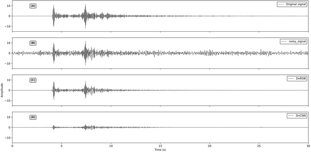
FIGURE 6. Comparison of denoising results of DnCNN and DnRDB on the same signal. (A) is original signal;(B) is noisy signal;(C) is DnCNN denoising result;(D) is DnRDB denoising result.

Noise Reduction Analysis of Different Kinds of Noise

In the process of seismic monitoring, the performance of the network is tested using some of the different kinds of noise. (Figure 7) depicts narrow-band noise, which has a strong frequency in a narrow range and always carries an accompanying signal. The DnRDB can identify and remove the noise for a variety of frequency bands. (Figure 8) shows low-frequency noise, the presence of which can result in strong fluctuations in seismic signals. It can be seen that the fluctuations it causes can be effectively suppressed by the DnRDB model. (Figure 9) illustrates high-frequency noise, which has a high main frequency band and a high amplitude. High-amplitude noise has a negative influence on the accuracy of event detection, but the DnRDB model can remove it effectively. Broadband noise, as shown in (Figure 10), has a wide frequency range, covering all the frequency ranges of seismic signals and also including nonseismic signals. The DnRDB model can accurately identify the former and remove the latter. (Figure 11) denotes spike pulse noise, the presence of which in seismic signals influences the extraction of the seismic phase and arrival time. Again, the DnRDB can remove spike pulse noise accurately. The noise in (Figure 12) has no fixed frequency band and no constant amplitude. The DnRDB model can recognize such complex noise and remove it from noisy seismic signals. It can therefore be seen from these figures that the DnRDB model can deal effectively with all kinds of noise. For a single type of noise, it can generally increase the SNR by more than 10 dB, with the correlation coefficient increasing to more than 0.95. This indicates that the DnRDB model is able to remove various forms of noise and improve the SNR of seismic signals while retaining the waveform shape of the signal. Not only can it remove a single type of noise, but it can also remove multiple types simultaneously. As shown in (Figure 11), when the signal contains both spike pulse and low-frequency noise, the model can remove both.

FIGURE 7

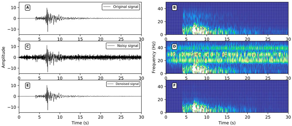
FIGURE 7. Narrow-band noise reduction performance. (A,C,E) are the original signals, the noise signal, and the signal after noise reduction in the time domain; (B,D,F) are the time-frequency domain data of (A,C,E); the signal SNR after adding noise = 0.50 dB, r = 0.7087, SNR after noise reduction = 16.54 dB, r = 0.9899.

FIGURE 8

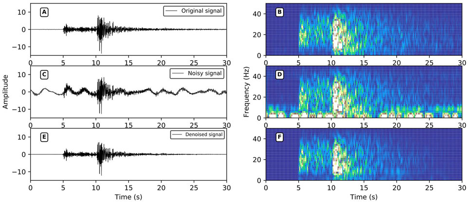
FIGURE 8. Low-frequency noise reduction performance. (A,C,E) are the original signals, the noise signal, and the signal after noise reduction in the time domain; (B,D,F) are the time-frequency domain data of (A,C,E); the signal SNR after adding noise = 0.21 dB, r = 0.7011, SNR after noise reduction = 12.84 dB, r = 0.9778.

FIGURE 9

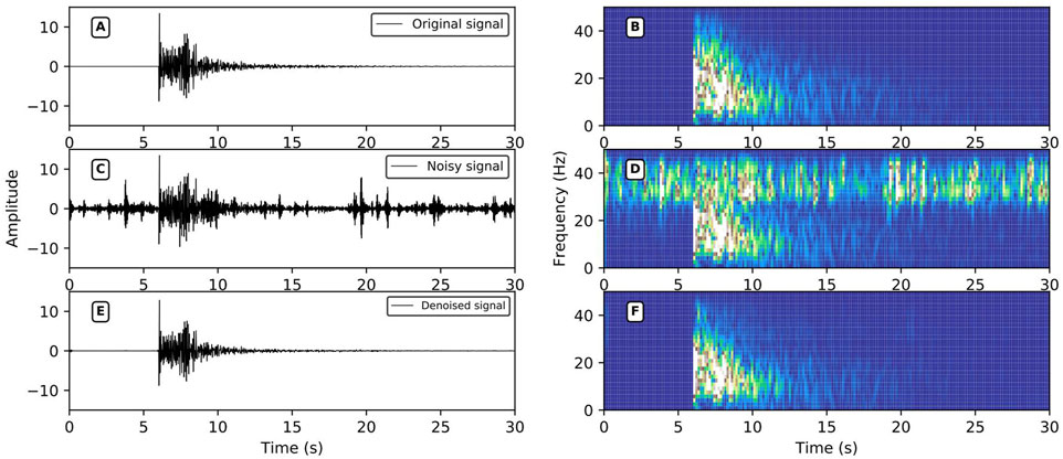
FIGURE 9. High-frequency noise reduction performance. (A,C,E) are the original signals, the noise signal, and the signal after noise reduction in the time domain; (B,D,F) are the time-frequency domain data of (A,C,E); the signal SNR after adding noise = −0.11 dB, r = 0.6961, SNR after noise reduction = 15.22 dB, r = 0.9861.

FIGURE 10

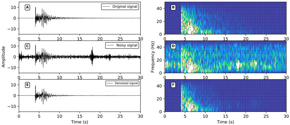
FIGURE 10. Broadband noise reduction performance. (A,C,E) are the original signals, the noise signal, and the signal after noise reduction in the time domain; (B,D,F) are the time-frequency domain data of (A,C,E); the signal SNR after adding noise = −0.52 dB, r = 0.6902, SNR after noise reduction = 9.78 dB, r = 0.9595.

FIGURE 11

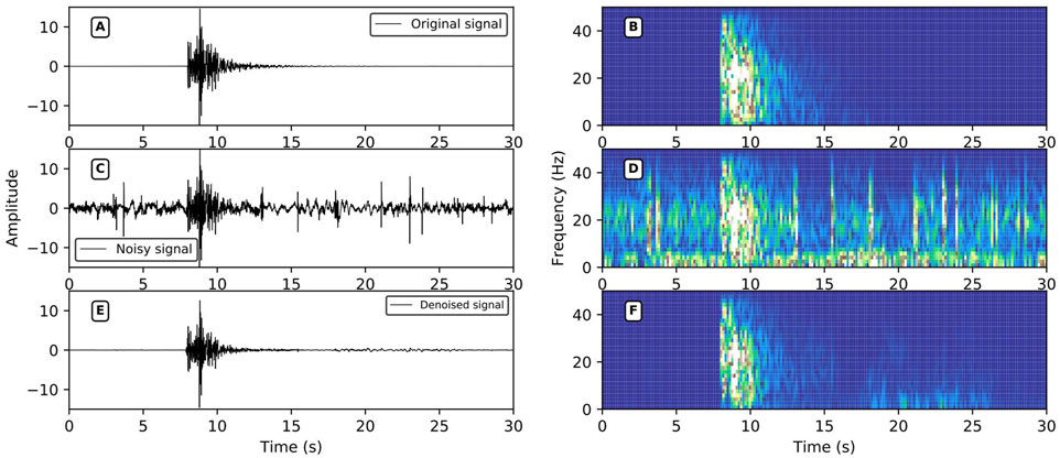
FIGURE 11. Spike noise reduction performance. (A,C,E) are the original signals, the noise signal, and the signal after noise reduction in the time domain; (B,D,F) are the time-frequency domain data of (A,C,E); the signal SNR after adding noise = 0.01 dB, r = 0.7013, SNR after noise reduction = 10.02 dB, r = 0.9578.

FIGURE 12

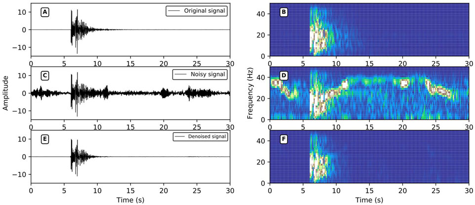
FIGURE 12. Other types of noise reduction performance. (A,C,E) are the original signals, the noise signal, and the signal after noise reduction in the time domain; (B,D,F) are the time-frequency domain data of (A,C,E); the signal SNR after adding noise = 0.34 dB, r = 0.7125, SNR after noise reduction = 13.07 dB, r = 0.9822.

Comparison With Other Methods

In order to further evaluate the denoising performance of the DnRDB model, we compared it with the other three denoising methods; wavelet threshold, EMD, and the DeepDenoiser model. The SNR and correlation coefficient were again adopted as evaluation indicators. We used the same test dataset, the criteria for selection being seismic signals with high SNR and random noise with a wide bandwidth. The selected data length was 3,000 sampling points. The selected seismic signals and noise waveforms are shown in (Figure 13). The noise and seismic signals were synthesized into noise-enhanced seismic signals with SNR of −6, −4, −2, 0, 2, 4, 6, 8, and 10 dB. The results of using the different denoising algorithms are shown in (Table 2).

FIGURE 13

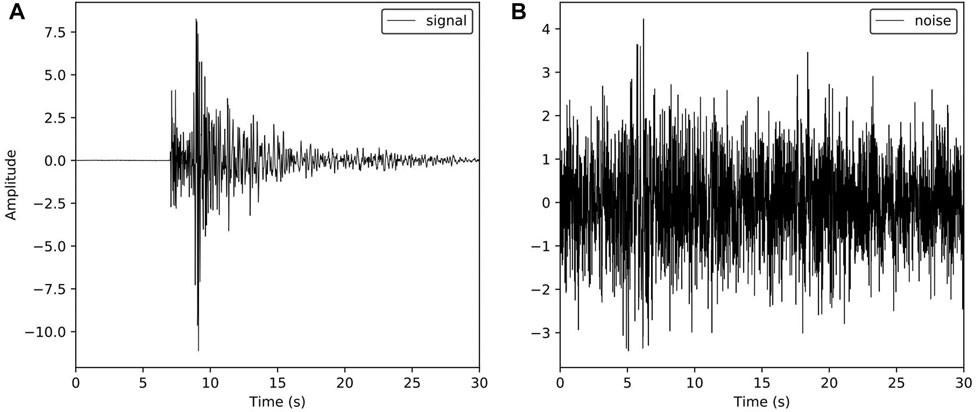
FIGURE 13. High SNR seismic signal and noise signal waveform; (A) seismic signal; (B) noise waveform.

TABLE 2

TABLE 2. Comparison of the denoising effects of different algorithms for different SNR.

In terms of (Table 2), compared with the wavelet threshold and EMD methods, the DnRDB model produces relatively higher SNR and correlation coefficients under different noise levels. In comparison with DeepDenoiser, both have a good denoising effect. Although there is a small gap in the SNR improvement achieved by the DnRDB model when the SNR of the noisy signal is higher than 4 dB, it is able to obtain a higher SNR; the average SNR of the output is also relatively high when the SNR of the noisy signal is low. For different noise levels, the correlation coefficient of the DnRDB model is higher than that of DeepDenoiser, indicating that it not only achieves a higher level of noise reduction, but also results in less waveform distortion. In summary, compared with the other three methods, the SNR and correlation coefficient of the DnRDB denoising results indicate a significant overall improvement and a higher denoising ability. This shows that the DnRDB model can improve the level of seismic signal denoising by fully extracting the features of seismic signals using the RDB module. Relative to the average SNR, the DnRDB model improves SNR by 3.22, 2.93, and 0.12 dB compared with the wavelet threshold, EMD, and DeepDenoiser methods, respectively. The average correlation coefficients increase respectively by 0.1049, 0.0832, and 0.0093.

(Figure 14) shows the waveform after noise reduction using various methods when the SNR of the noise-added signal is 4 dB. As can be seen, the denoising results of the wavelet threshold and EMD are relatively poor. While DeepDenoiser has a better effect, some noise has not been removed before the signal P arrives at the time point. The denoised signal of the DnRDB model contains the least noise residue of all the tested models, especially before the signal P arrival, which is helpful for the detection of subsequent seismic events and phases.

FIGURE 14

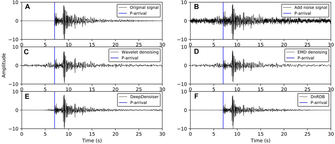
FIGURE 14. Waveform comparison of the noise reduction results of various methods for SNR of 4dB. (A) Original data; (B) Noisy data; (C) Wavelet denoising result; (D) EMD denoising result; (E) DeepDenoiser denoising result; (F) Denoising result of the DnRDB model reported here.

Application of Seismic Signal Denoising—Seismic Phase Identification of Wenchuan Aftershocks

The presence of a large amount of noise in a seismic signal can have an influence on the detection algorithm. This is commonly applied to the acquisition of seismic phases and reduces the accuracy and recall rate of the recognition process. Accuracy indicates that the seismic phase picked up by the algorithm is within the error range and consistent with the reference phase. The recall rate illustrates the completeness of the time selected compared with a reference. For instance, the performance of the short-/long-term average (STA/LTA) seismic phase identification algorithm is easily affected by noise. (Figure 15) shows the recognition effect of the STA/LTA seismic phase before and after denoising using the DnRDB model. Figures 15A,B shows the waveforms of the seismic signals before and after noise reduction, Figure 15C the STA/LTA eigenfunction values of the original signal, and Figure 15D the STA/LTA eigenfunction values of the denoised signal. By comparing the eigenfunction values before and after noise reduction, it can be seen that these are more prominent and easier to identify for the denoised signal of both P and S to time point. Therefore, denoising seismic signals helps to improve the seismic phase identification ability of the algorithm. In order to test the practical impact of the DnRDB model for noise reduction, it was applied to the Wenchuan earthquake aftershock dataset from May to September 2008.

FIGURE 15

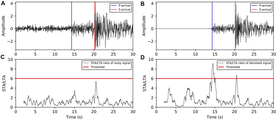
FIGURE 15. Comparison of the seismic phase recognition effect before and after denoising; (A) seismic signal before noise reduction; (B) signal after DnRDB noise reduction; (C) the eigenfunction of the STA/LTA before noise reduction; (D) the eigenfunction of the STA/LTA after noise reduction.

Data Sharing Infrastructure of National Earthquake Data Center (http://data.earthquake.cn). This dataset consists of a total of 2026 seismic phase data from 76 stations, including seismic events and related seismic phase data. The signal in the dataset was resampled to 100 Hz, and the length of the intercepted waveform set at 30 s. The SNR level of the dataset before noise reduction was between 2 and 5 dB, and that after noise reduction by the DnRDB was between 7 and 11 dB. (Table 3) shows the recognition accuracy rates of Pg and Sg after noise reduction were 70 and 77%, and the recall rates 79 and 84% respectively, representing a significant improvement through noise reduction. Therefore, the DnRDB model can help improve the performance of the seismic phase recognition algorithm in practical applications.

TABLE 3

TABLE 3. Comparison of the seismic phase acquisition results of the original and denoised signals by STA/LTA.

Conclusion

In this paper, we have described the use of a convolutional deep network seismic signal denoising (DnRDB) model based on RDB to remove noise from the seismic waveform by using the noisy data to learn the complex features of seismic signals. The network utilizes the RDB module as the basic component, which can fully extract the characteristics of seismic signals and improve their SNR. The results of testing the model on noisy seismic waveform data illustrates that this method has good denoising ability for various types of seismic noise. Compared with traditional denoising methods and other deep learning methods, the DnRDB model can achieve higher average SNR and correlation coefficient. When the model is applied in practice to seismic data, it can lead to improved seismic phase recognition ability through noise reduction.

Although this method achieved a good level of noise reduction, some shortcomings still deserve attention. Firstly, due to resource constraints, the number of convolution layer feature maps and RDB modules used in the DnRDB model reported here is relatively small. Increasing the number of layers and the size of the model could improve its performance to a certain extent. Secondly, this was a supervised model and so strongly reliant on clean seismic data; however, clean seismic waveforms cannot be obtained, which limits the denoising ability of the neural network.

Data Availability Statement

The original contributions presented in the study are included in the article/Supplementary Material, further inquiries can be directed to the corresponding author.

Author Contributions

ZG analyzes data and proposes methods; SZ perfects the model and writes manuscripts; JC proposes and participates in design research and reviews papers; LH improves and perfects papers; JZ participates in model experiment. All the authors approved the final version of the manuscript.

Funding

This work was supported by Scientific Research Project Item of Hebei Province Education Department (Grant No. QN2018317), The National Key Research and Development Program of China (Grant No. 2018YFC1503801), and the Special Fund of Fundamental Scientific Research Business Expense for Higher School of Central Government (Grant No. ZY20180111).

Conflict of Interest

The authors declare that the research was conducted in the absence of any commercial or financial relationships that could be construed as a potential conflict of interest.

Acknowledgments

Acknowledgement for the data support from “China Earthquake Networks Center, National Earthquake Data Center. (http://data.earthquake.cn).

References

Bekara, M., and Baan, M. (2011). Random and Coherent Noise Attenuation by Empirical Mode Decomposition. Geophysics 74 (5), V89–V98. doi:10.1190/1.3157244

CrossRef Full Text | Google Scholar

Cao, S., and Chen, X. (2005). The Second-Generation Wavelet Transform and its Application in Denoising of Seismic Data. Appl. Geophys. 2 (2), 70–74. doi:10.1007/s11770-005-0034-4

CrossRef Full Text | Google Scholar

Chen, Y., and Ma, J. (2014). Random Noise Attenuation by F-X Empirical-Mode Decomposition Predictive Filtering. Geophysics 79 (3), V81–V91. doi:10.1190/geo2013-0080.1

CrossRef Full Text | Google Scholar

Dong, X., Zhong, T., and Li, Y. (2020). A deep-learning-based denoising method for multiarea surface seismic data. IEEE Geoscience and Remote Sensing Letters, (99), 1–5. doi:10.1109/LGRS.2020.2989450

CrossRef Full Text | Google Scholar

Gaci, S. (2014). The Use of Wavelet-Based Denoising Techniques to Enhance the First-Arrival Picking on Seismic Traces. IEEE Trans. Geosci. Remote Sensing 52 (8), 4558–4563. doi:10.1109/tgrs.2013.2282422

CrossRef Full Text | Google Scholar

Han, J., and van der Baan, M. (2015). Microseismic and Seismic Denoising via Ensemble Empirical Mode Decomposition and Adaptive Thresholding. Geophysics 80 (6), KS69–KS80. doi:10.1190/geo2014-0423.1

CrossRef Full Text | Google Scholar

Huang, G., Liu, Z., Laurens, V., and Weinberger, K. Q. (2016). 2017 IEEE Conference on Computer Vision and Pattern Recognition (CVPR). IEEE, Honolulu, HI, 2261–2269. doi:10.1109/CVPR.2017.243

Huang, N. E., Shen, Z., Long, S. R., Wu, M. C., Shih, H. H., Zheng, Q., et al. (1998). The Empirical Mode Decomposition and the hilbert Spectrum for Nonlinear and Non-stationary Time Series Analysis. Proc. R. Soc. Lond. A. 454 (1971), 903–995. doi:10.1098/rspa.1998.0193

CrossRef Full Text | Google Scholar

Huang, P. S., Kim, M., Hasegawa-Johnson, M., and Smaragdis, P. (2014). “Deep Learning for Monaural Speech Separation,” in IEEE International Conference on Acoustics, Florence, Italy, 4-9 May 2014 (IEEE). doi:10.1109/icassp.2014.6853860

CrossRef Full Text | Google Scholar

Huang, P. S., Kim, M., Hasegawa-Johnson, M., and Smaragdis, P. (2015). Joint Optimization of Masks and Deep Recurrent Neural Networks for Monaural Source Separation. IEEE/ACM Trans. Audio Speech Lang. Process. 23 (12), 2136–2147.

Google Scholar

Ioffe, S., and Szegedy, C. (2015). “Batch Normalization: Accelerating Deep Network Training by Reducing Internal Covariate Shift,” in The 32nd International Conference on Machine Learning (ICML 2015), July 6–11, 2015, Lille, France, 448–456.

Google Scholar

Jin, Yuchen., Wu, Xuqing., Chen, Jiefu., Han, Zhu., and Hu, Wenyi. (2018). “Seismic Data Denoising by Deep-Residual Networks,” in 2018 SEG International Exposition and Annual Meeting, 14-19 October 2018, Anaheim, CA. doi:10.1190/segam2018-2998619.1

CrossRef Full Text | Google Scholar

Kim, D. W., Ryun Chung, J., and Jung, S. W. (2019). “GRDN: Grouped Residual Dense Network for Real Image Denoising and gan-based Real-World Noise Modeling,” in Proceedings of the IEEE/CVF Conference on Computer Vision and Pattern Recognition Workshops, 15-20 June 2019, Long Beach, CA, 0.

Google Scholar

Krizhevsky, A., Sutskever, I., and Hinton, G. (2012). ImageNet Classification with Deep Convolutional Neural Networks. NIPS, 25, December 3-8, Harrahs and Harveys, Lake Taho. Curran Associates Inc.

Li, S., Zhao, M., Fang, Z., Zhang, Y., and Li, H. (2020). Image Super-resolution Using Lightweight Multiscale Residual Dense Network. Int. J. Opt. 2020, 1–11. doi:10.1155/2020/2852865

CrossRef Full Text | Google Scholar

Mao, X. J., Shen, C., and Yang, Y. B. (2016). Image Restoration Using Convolutional Auto-Encoders with Symmetric Skip Connections. arXiv preprint arXiv:1606.08921.

Google Scholar

Ming-Yue, , and Zhai, (2014). Seismic Data Denoising Based on the Fractional Fourier Transformation. J. Appl. Geophys. 109, 62–70. doi:10.1016/j.jappgeo.2014.07.012

CrossRef Full Text | Google Scholar

Mousavi, S. M., Langston, C. A., and Horton, S. P. (2016). Automatic Microseismic Denoising and Onset Detection Using the Synchrosqueezed Continuous Wavelet Transform. Geophysics 81 (4), V341–V355. doi:10.1190/geo2015-0598.1

CrossRef Full Text | Google Scholar

Mousavi, S. M., Sheng, Y., Zhu, W., and Beroza, G. C. (2019). STanford EArthquake Dataset (STEAD): A Global Data Set of Seismic Signals for AI, 99. IEEE Access, 1.

Nair, Vinod., and Hinton, Geoffrey. E. (2010). “Rectified Linear Units Improve Restricted Boltzmann Machines.” In The 27th International Conference on Machine Learning (ICML 2010), June 21-24, 2010, Haifa, Israel, 807–814.

Google Scholar

Ronneberger, O., Fischer, P., and Brox, T. (2015). U-net: Convolutional Networks for Biomedical Image Segmentation. International Conference on Medical Image Computing and Computer-Assisted Intervention, October 5-9, 2015, Munich, Germany. Cham: Springer.

Google Scholar

Weninger, F., Eyben, F., and Schuller, B. (2014). Single-channel Speech Separation with Memory-Enhanced Recurrent Neural Networks. Florence, Italy: IEEE. doi:10.1109/icassp.2014.6854294

CrossRef Full Text

Yu, S., Ma, J., and Wang, W. (2018). Deep Learning Tutorial for Denoising. Geophysics 84 (6), V333–V350. doi:10.1190/igc2018-113

CrossRef Full Text

Zhang, K., Zuo, W., Chen, Y., Meng, D., and Lei, Z. (2016). Beyond a Gaussian Denoiser: Residual Learning of Deep Cnn for Image Denoising. IEEE Trans. Image Process. 26 (7), 3142–3155. doi:10.1109/TIP.2017.2662206

Google Scholar

Zhang, Y., Lin, H., Li, Y., and Ma, H. (2019). A Patch Based Denoising Method Using Deep Convolutional Neural Network for Seismic Image, 7. IEEE Access, 156883–156894. doi:10.1109/access.2019.2949774

CrossRef Full Text

Zhang, Y, Tian, Y, Kong, Y, Zhong, B, and Fu, Y. (2021). Residual Dense Network for Image Restoration. IEEE Trans Pattern Anal. Mach Intell. 2020 Jul; 43 (7): 2480–2495. doi:10.1109/TPAMI.2020.2968521

Google Scholar

Zhang, Y., Tian, Y., Kong, Y., Zhong, B., and Fu, Y. (2018). Residual Dense Network for Image Super-resolution 43. Salt Lake City, UT: IEEE. doi:10.1109/cvpr.2018.00262

CrossRef Full Text

Zhang, Zongbao., and Cai, L. I. U. (2014). Application of Fractional Fourier Transform in Seismic Data Denoising. Glob. Geology. 17 (2), 110–114.

Google Scholar

Zhu, W., Mousavi, S. M., and Beroza, G. C. (2019). Seismic Signal Denoising and Decomposition Using Deep Neural Networks. IEEE Trans. Geosci. Remote Sensing 57 (11), 9476–9488. doi:10.1109/TGRS.2019.2926772

Google Scholar