 Yushan Xie
 Ruyi Zhang
 Zhipeng Zhu
 Limin Zhou
94% of researchers rate our articles as excellent or good
Learn more about the work of our research integrity team to safeguard the quality of each article we publish.
Find out more
ORIGINAL RESEARCH article
Front. Earth Sci., 16 June 2021
Sec. Atmospheric Science
Volume 9 - 2021 | https://doi.org/10.3389/feart.2021.673808
This article is part of the Research TopicAtmospheric ElectricityView all 12 articles
Global electric circuits could be the key link between space weather and lower atmosphere climate. It has been suggested that the ultrafine erosol layer in the middle to upper stratosphere could greatly contribute to local column resistance and return current density. In previous work by Tinsley, Zhou, and Plemmons (Atmos. Res., 2006, 79 (3–4), 266–295), the artificial ultrafine layer was addressed and caused a significant symmetric effect on column resistance at high latitudes. In this work, we use an updated erosol coupled chemistry-climate model to establish a new global electric circuit model. The results show that the ultrafine aerosol layer exits the middle stratosphere, but due to the Brewer-Dobson circulation, there are significant seasonal variations in the ion loss due to variations in the ultrafine aerosol layer. In the winter hemisphere in the high latitude region, the column resistance will consequently be higher than that in the summer hemisphere. With an ultrafine aerosol layer in the decreasing phase of solar activity, the column resistance would be more sensitive to fluctuations in the low-energy electron precipitation (LEE) and middle-energy electron precipitation (MEE) particle fluxes.
The global atmospheric electric circuit could be important not only as a product of global thunderstorm activity (Bering et al., 1998) but also because it may cause climate change and weather itself via electrical effects on cloud microphysics, with external and internal drivers (Tinsley and Yu, 2004; Tinsley, 2008), which depend on the current density Jz flowing downwards from the ionosphere to the surface through clouds. This hypothesis has been reviewed in detail by Tinsley (2008).
The ionosphere forms a conducting shell, which is charged by highly electrified clouds, including thunderclouds in low latitude regions and air fronts at middle and high latitudes. The diurnal variations in the global upward current of approximately 1000 A create a diurnally varying ionospheric potential (Vi) that averages approximately 250 kV, which is essentially an equipotential out to approximately 50° geomagnetic latitudes. At any location away from the generators, the downward return current density (Jz) is 1–6 pA m-2, depending on the atmospheric resistance R of the column of the unit cross section there. The vertical column resistance R at any location is mainly determined by the altitude of the surface, the aerosol, the cloud and radioactive radon concentrations near the surface, and the flux of galactic cosmic rays (GCRs) at that latitude (Tinsley et al., 2006). The GCR flux creates ion pairs throughout the air column, increasing ion pairs cause the increase of conduct, leading to stronger Jz. There are two additional sources of ion pair production in the upper atmosphere: one is the relativistic electron flux and associated X-ray bremsstrahlung that penetrates down to approximately 30 km in sub-auroral latitudes (Tinsley, 1996; Frahm et al., 1997; Li et al., 2001a, b), and the other is solar energetic particle (SEP) events (Holzworth et al., 1987) that produce stratospheric ionization, excess positive charge, and occasionally a small amount of tropospheric ionization in the polar cap regions. We denote the stratospheric and tropospheric contributions to the column resistance at any location as S and T, respectively. Then Jz at that location is given by Ohm’s Law:
It was proposed that the reduction in Jz due to the Forbush decrease in GCRs could be attributed to the latitudinal variations in the low atmospheric dynamics, represented by the vorticity area index (VAI), and the amplitude of the response was proportional to the amplitude of the Forbush decrease (Tinsley and Deen, 1991). Other studies claimed that the relationship between Jz and VAI was due to the internal variation of the thunderstorm (Hebert et al., 2012) or interplanetary magnetic field (IMF) (Wilcox et al., 1973; Lam and Tinsley, 2016; Zhou et al., 2018). Responses of cloud cover to heliospheric current sheet (HCS) crossings have been found by Kniveton et al. (2008) and to Forbush decreases by Veretenenko and Pudovkin (1997), and responses of global cloud cover to global Jz changes inferred from the electric field (Ez) measurements at Vostok have been found by Kniveton et al. (2008). On longer time scales, the relation between the relativistic electron flux and the pressure fluctuation in the winter ice island pressure center is important (Zhou et al., 2014). These responses between space weather and atmospheric parameters were more significant two or three years after large volcanic eruptions, such as the eruption of Mt. Aguge, Mt. El Chikon, and Mt. Pinatubo, which was proposed to be due to additional resistance by the ultrafine aerosol layer in the stratosphere (Tinsley and Yu, 2004; Zhou et al., 2014). It has been suggested that after a large volcanic eruption, the gaseous H2SO4 in the descending branch of the Brewer-Dobson circulation could be condensed by ion media nucleation and form large concentrations of ultrafine aerosols with radii of a few nanometers or tens of nanometers at mid-high latitudes, which could significantly increase the column resistance in the stratosphere.
The initial evaluation of this effect was performed by the global circuit model of TZ06 (Tinsley et al., 2006). In the TZ06 model, an ultrafine aerosol layer was modeled by Tinsley et al. (2006), where column resistance is mainly shown in situations with and without the estimated stratospheric ultrafine volcanic aerosol layer. The layer is located poleward of ±40° geographic latitudes, where the layer column resistance becomes the dominant part of the stratosphere and is calculated for the absence of ionization due to electron precipitation, such as relativistic electron flux. This ionization is considered to be present most of the time and to make the ultrafine layer a good conductor so that the column resistance in the stratosphere (S) is negligible with respect to that in the troposphere (T). It is only for periods of a few days when the slow solar wind at the HCS crosses the earth that the precipitating relativistic electron flux decreases by an order of magnitude; R increases and Jz decreases at higher latitudes during a few years following large explosive volcanic eruptions. The concentration and spatial distribution of stratospheric ultrafine aerosols in TZ06 are artificial and static with no temporal variation, which provides only a rough estimation of their effects. The improved comprehensive model of BTNL 2013, based on CESM1, where the sulfate aerosol process in the stratosphere is from English et al. (2011), includes all types of aerosols, including ultrafine aerosols due to ion media nucleation in the stratosphere, and provides a more realistic picture of the global circuit. However, the lack of heating as aerosol radiative feedback in English et al. (2011) causes a large bias in the aerosol burden between simulations and observations. The improved aerosol-chemistry-climate model SOCOL-AERv2 by Feinberg et al. (2019) can already provide a more accurate treatment of stratosphere aerosols for low and high volcanic periods with aerosol radiative heating, sedimentation schemes, and coagulation efficiency. The purpose of this work is to investigate the effect of the stratospheric aerosol layer on the column resistance with the comprehensive global electric circuit model, which is based on SOCOL-AERv2 coupled with the global electric model of TZ06, where ultrafine aerosols due to ion media nucleation are involved to more accurately evaluate the effect of ultrafine aerosols and the temporal variation in this effect. In addition, the effects of ionization due to galactic cosmic rays and high-energy electron precipitation are addressed.
The chemistry-climate model (CCM) SOCOL (SOlar Climate Ozone Links) version three is a three-dimensional model developed by the research group at the Physical-Meteorological Observatory and World Radiation Center (PMOD/WRC) in collaboration with the Institute for Atmospheric and Climate Science, ETHZ Switzerland (Stenke et al., 2013). The effects of external drivers, such as galactic cosmic rays and solar protons, on the ozone layer and climate were investigated by the SOCOL model (Egorova et al., 2011; Mironova et al., 2021). A detailed description of the model can be found in Rozanov et al. (1999).
SOCOL is developed based on the Middle Atmosphere version of the European Center/Hamburg Model version 5 (MA-ECHAM5). MA-ECHAM5 (Roeckner et al., 2003) is the dynamical core of the model responsible for atmospheric physics and dynamics in SOCOL, with a hybrid sigma-pressure coordinate system spanning from the surface to 0.01 hPa. The horizontal spatial resolution of the model in this work is 3.75 × 3.75°. The model has 39 vertical levels from the surface to a height of approximately 80 km in a hybrid sigma-pressure coordinate system, and the vertical resolution decreases with altitude and is 2 km in the stratosphere. The dynamic frame in the model is solved with a semi-implicit time stepping scheme with a time resolution of 15 min. The advection of water vapor, cloud water, and trace constituents is calculated by a flux-based 25 mass-conserving and shape-preserving transport scheme (Lin and Rood, 1996). Full radiation calculations, chemistry, and transport calculations are performed every 2 h. The shortwave radiation scheme is based on the ECMWF model (Morcrette, 1991) with a modified parameterization for the water vapor continuum and corrected spectral Voigt line shape considering Doppler broadening at low pressure as well as with added aerosols, greenhouse gases, and clouds (Roeckner, 1995). The longwave radiation is based on the Rapid Radiative Transfer Model (RRTM) scheme (Mlawer et al., 1997).
The chemistry-transport module Model for the Evaluation of OZONe Trends (MEZON) (Egorova et al., 2003) shares the MA-ECHAM5 horizontal and vertical grids and treats 41 atmospheric species of hydrogen, oxygen, nitrogen, carbon, chlorine, and bromine groups treated with 140 gas-phase reactions, 46 photolysis reactions, and 16 heterogeneous reactions in/on liquid sulfate aerosols, water ice, and nitric acid trihydrate (NAT) (Stenke et al., 2013).
The ion pair production rate due to galactic cosmic rays is calculated by the CRAC (Cosmic Ray Atmospheric Cascade) model (Usoskin et al., 2010), which is based on a Monte Carlo simulation of the atmospheric cascade; in the troposphere and stratosphere, the accuracy is within 10% compared to the observation results. In the present work, we also add the ion pair due to low- and middle-energy electron precipitation (herein EEP, including LEE and MEE). The semi-empirical parameterization for LEE suggested by Funke et al. (2016) is involved, and the ionization rate due to MEE is based on Fang et al. (2010).
In the troposphere, 13 types of aerosols based on the GADS database and Hess et al. (1998) are involved, which is the same as the treatment in the TZ06 model. We use an analytical expression for the tropospheric aerosol size distribution given by Hess et al. (1998).
For the sulfate aerosol in the model, instead of the rough estimation that was used in TZ06, a detailed 2D sulfate aerosol model is coupled based on the updated size-resolved AER sulfate aerosol model, which was established in SOCOL by Sheng et al. (2015), Sukhodolov et al. (2018), and Feinberg et al. (2019). In this sulfate aerosol model, the particle distribution is resolved by 40 size bins spanning wet radii from 0.39 nm to 3.2 µm by volume doubling, which also provides the size distribution of the sulfate aerosol. In addition, the microphysical processes of homogeneous nucleation, condensation/evaporation, coagulation, and sedimentation, which were suggested by Sheng et al. (2015), are also included. In the upper stratosphere at altitudes over 30 km, the coagulation rate due to ion media nucleation is addressed in this new model, which is based on the INM model suggested by Yu and Turco (2001).
The column resistance (R) varies with latitude and longitude, and with the upper boundary of 60 km in our model, R is given by
where Zs is the elevation of the surface and σ(z) is air conductivity. The current density Jz throughout the column is then
where Vi is the overhead ionospheric potential. The most complex problem for this global circuit model is in evaluating σ(z) globally as a function of altitude, latitude, longitude, and time.
In this model, the first step is the evaluation of the ion pair production rate; the next step is the evaluation of the aerosol particle concentrations. Then, using the approximation that the concentrations of positive and negative ions in the air are equal, the ion pair concentration (n) is obtained by solving the equation
for the steady state condition where dN/dt = 0, where t is the time. Then, the conductivity is given by
where e is the elementary charge, and
We use a set of expressions for α that closely fit the results of Bates (1982). The expression for βr as a function of aerosol particle radius, r, that we use is given by Hoppel (1985).
The present global electric circuit model calculates the atmospheric resistivity from the surface up to 60 km height with 335 bins. We took only 32 vertical bins below 60 km in the SOCOL-AERv2 model, all the outputs from the SOCOL-AERv2 model are linearly interpolated, and the sulfate gas concentration and sulfate aerosol surface area index (surface area density, SAD) are interpolated with the e power function.
Figure 1 compares the simulation results of the SO2 mixing ratio from SOCOL-AER at 26–32°N in April to May 1985 with MIPAS and ATMOS observed data (Höpfner et al., 2013; Rinsland et al., 1995). There are a number of similarities between the simulation results and satellite measurements. The estimated instrumental uncertainty of MIPAS is 5–10 pptv (Höpfner et al., 2013). Differences between observed data and simulation data below 45 km are less than 10°pptv. This result is similar to Sheng et al. (2015), who found that SOCOL-AER could successfully simulate aerosol features.
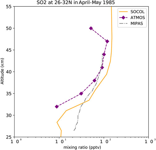
FIGURE 1. Comparison of the SO2 mixing ratio at 26–32°N in april to May 1985 simulated by SOCOL-AER (orange solid line), from ATMOS observations (purple squares) and from MIPAS measurements (gray dashes).
As shown in Figure 2, during 1990–1993, the Brewer-Dobson circulation exhibited significant seasonal variations. The top half of the figure shows circulation characteristics during summer; at nearly 30 km, the residual velocity at high latitudes decelerated in 1990 and 1992 but accelerated in 1991. The bottom half of Figure 2 shows that near 30 km, the residual velocity at high latitudes accelerated the upper polar region during the 1990–1992 winter but decelerated in 1993.
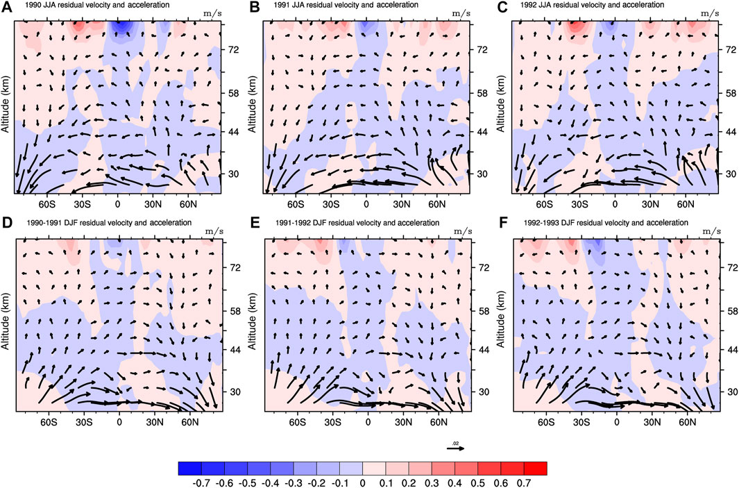
FIGURE 2. The residual speed and acceleration in the summer (first row) and winter (second row) from 1990 to 1993. The colored diagram is acceleration, and the vector arrow is the composite of vertical wind and meridional wind (
Figures 3A–D show the ion pair production rate at standard temperature and pressure (STP) for particles with different energies during solar maxima and solar minima: 1) is for ion pair production rate due to GCRs during the solar minimum, 2) is for the ion pair production rate due to GCRs during the solar maximum, 3) is for the ion production rate due to GCRs + EEP during the solar minimum, and 4) is for the ion production rate due to GCRs + EEP during the solar maximum. This shows that the ion production rate during solar minima at an altitude of 60 km in the polar region due to ionization of GCRs and EEP could be twice that during solar maxima, and at 30 km, the ion production rate is enhanced by an additional 1.15 due to EEP. During solar maxima, the difference at an altitude of 60 km is less than 10%. Therefore, additional EEP ionization was significantly attributed to ion production above a height of 30 km in the polar region.
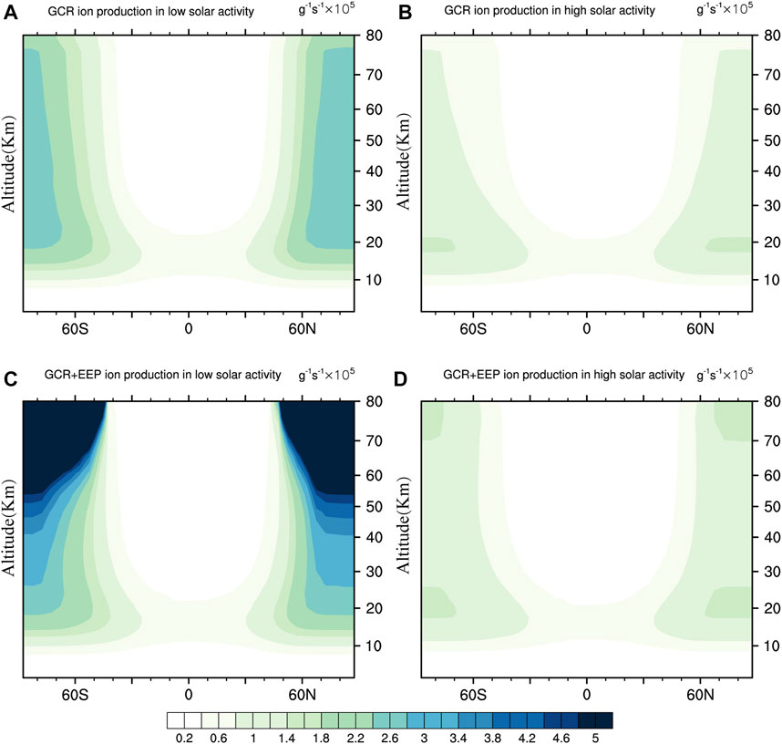
FIGURE 3. The ion pair production rate due to GCRs and EEP. (A) shows the ion pair production rate due to GCRs during the solar minimum, (B) shows the ion pair production rate due to GCRs during the solar maximum, (C) shows the ion production rate due to GCRs + EEP during the solar minimum, and (D) shows the ion production rate due to GCRs + EEP during the solar maximum.
With the SOCOL-AERv2 model, a more accurate simulation of sulfate aerosol concentration was achieved. In general, there are two sulfate aerosol layers after a volcanic eruption: one is in the troposphere, and the other is in the low stratosphere layer, which is well known as the “Junge layer” (Junge and Manson, 1961). Yu and Turco (2001) and Tinsley (2005) suggested that there was a third layer in the middle to upper stratosphere due to ultrafine sulfate aerosols. Therefore, Figure 4 shows the sulfate aerosol-related parameters in the middle to upper stratosphere. Figure 4 shows the zonal mean SAD (panels a and b) and sulfate mass concentration (panels c and d) as a function of altitude above 23 km. Figures 4A,C show the results in December-January-February (DJF) 1992–1993 after the eruption of Mt. Pinatubo, and Figures 4B,D show the results in DJF 1990–1991 just before the eruption of Mt. Pinatubo. The results show that there is significant enhancement of SAD and sulfate mass concentration in the middle stratosphere after the eruption of Mt. Pinatubo compared with the results in DJF 1990–1991 before the eruption. The most interesting aspect of Figures 4A,C is that the maxima of SAD and sulfate mass concentration over the high latitudes of the Northern hemisphere are in the region of Brewer-Dobson circulation in the descending branch. In Figures 2D,E there is a clear trend of residual velocity descent over the high latitudes of the Northern hemisphere at 30 km during the 1990–1992 winter. Compared to the estimation by Tinsley (2005) and Tinsley et al. (2006), the maximum SAD and sulfate mass concentrations are lower. They are centered at a height of approximately 30 km.
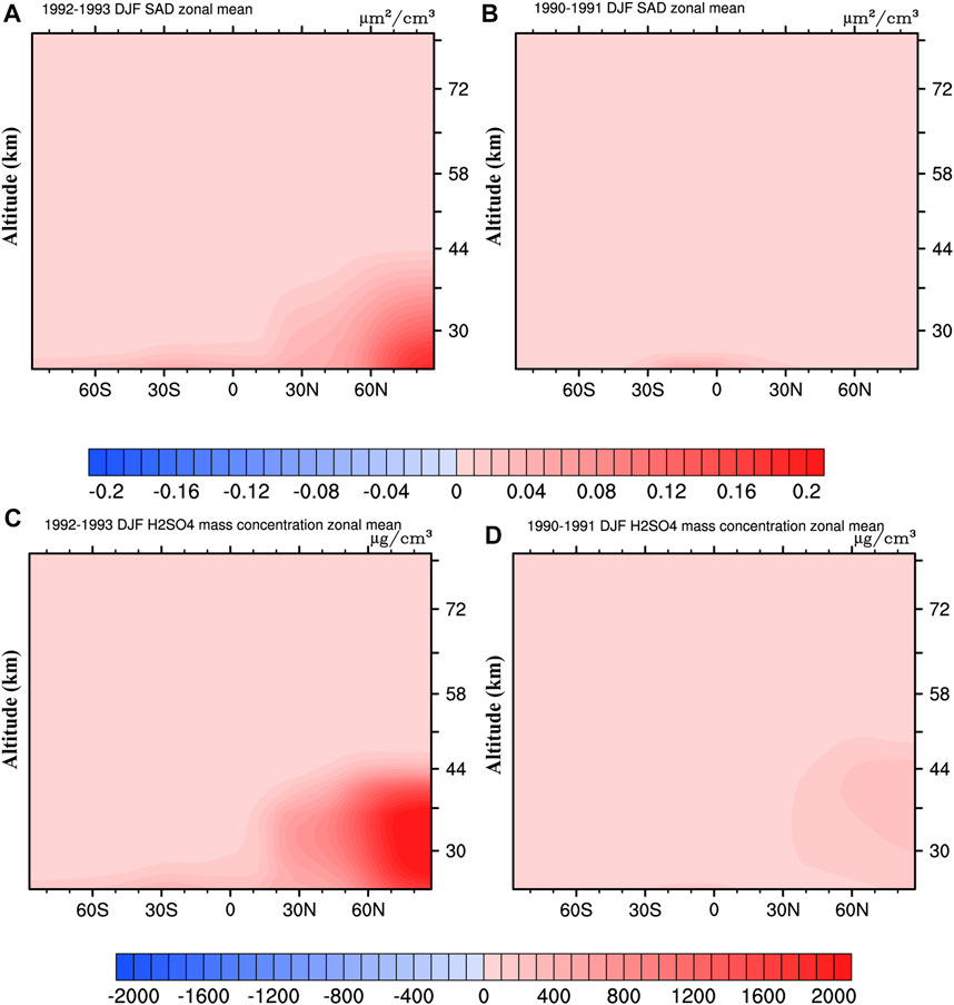
FIGURE 4. The characteristics of sulfate aerosols in the middle and upper stratosphere (panels (A) and (B)) and sulfate mass concentration (panels (C) and (D)) as a function of altitude above 23 km.
In the global electricity circuit model, ion loss due to ion-aerosol attachment is the main part of the whole ion loss. Figure 5 shows the profile of the ion-aerosol attachment rate (β) in two different regions (Antarctic 1) and Indian Ocean 2)) under different volcanic eruptions. In these two plots, the gray lines are the results from the TZ06 model, the gray solid line is the value in DJF with high volcanic aerosol loading, and the gray dashed line is the value in DJF with low volcanic aerosol loading. The black solid line is for DJF in 1990–1991, the black dashed line is for DJF in 1991–1992, and the red solid line is for June-July-August (JJA) in 1991. The results show that the ultrafine aerosol layer appears in only the high latitude region, which is consistent with previous studies. The ion loss due to attachment to ultrafine aerosols at low volcanic activity in the new model is approximately 20 times larger than that in the TZ06 model. The maximum ion loss due to attachment to sulfate aerosols exists at a height of 35 km, which is consistent with the vertical distribution of sulfate aerosols in Figure 4. After the large volcanic eruption, β is enhanced by approximately 3–4 times due to seasonal variations, which is not addressed in TZ06, ZT09, or other models. The ion loss due to attachment to aerosols in the Junge layer is also increased by a factor of approximately 10 compared with the TZ06 model. Although aerosol in the Junge layer also exhibited a peak value in polar and tropical regions after volcanic eruption, it was only 100 times less than the effect due to surface aerosols and ultrafine aerosols.
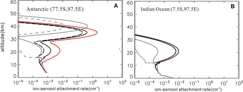
FIGURE 5. "Vertical profile of the ion-aerosol attachment rate (β) in two different regions (Antarctic (A) and Indian Ocean (B)) under different volcanic eruptions. In these two plots, the gray lines are the results from the TZ06 model, the gray solid line is the value in DJF with high volcanic aerosol loading, and the gray dashed line is the value in DJF with low volcanic aerosol loading. The black solid line is for DJF in 1990–1991, the black dashed line is for DJF in 1991–1992, and the red solid line is for JJA in 1991.
Figure 6 shows the ion-aerosol attachment rate at a height of 35 km in JJA 1993 and DJF 1993–1994. In the high-latitude region, there is a significant seasonal fluctuation in β, and the maximum variation is over 10 times.
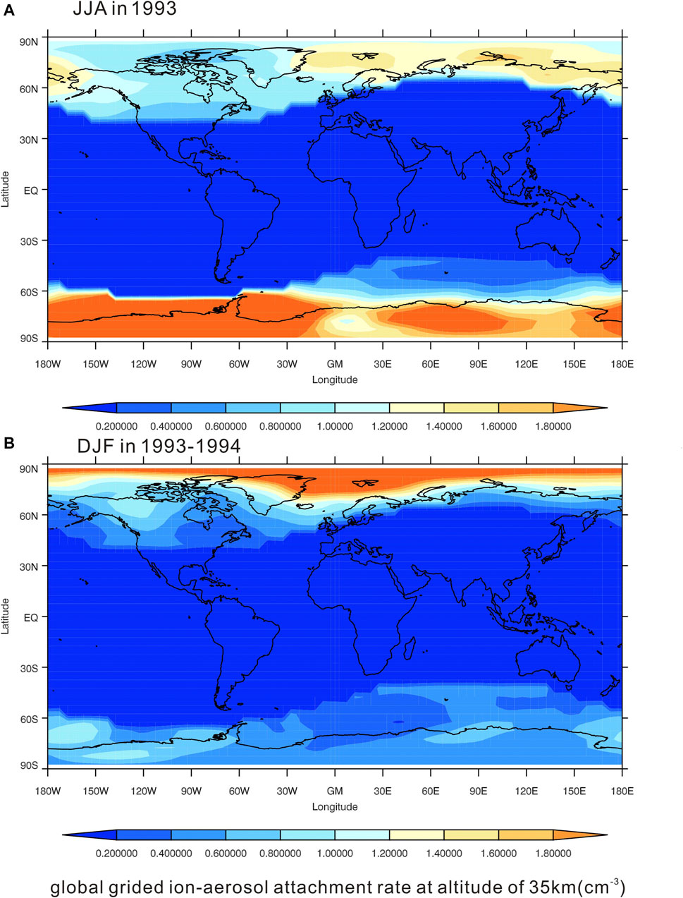
FIGURE 6. Global ion-aerosol attachment rate at a height of 35 km, (A) for JJA in 1993 and (A) for DJF in 1993–1994.
Figure 7 shows the vertical profiles of atmospheric resistivity in DJF in the 1) Antarctic and 2) Indian Ocean. The solid lines are for the 1990–1991 period, dotted lines are for the 1992–1993 period, and dashed lines are for the 1993–1994 period. In the high-latitude/Antarctic region, the effect of the Junge layer could not be detected, and ultrafine volcanic eruptions and resistivity at a 35 km height significantly contributed to the whole column resistance, especially after volcanic eruptions. The sulfate aerosol effect weakens with time. In the tropical Indian Ocean region, the peak resistivity was found at a height of 20 km, which is due to the Junge layer. However, the resistivity of the Junge layer is not large and does not significantly affect the whole column resistance value. It is apparent from Figure 8B that above the Indian Ocean air resistivity for the 1993–1994 period became almost the same as in pre-eruption time, a possible explanation for this might be that the effect and lifetime of ultrafine sulfate aerosols in the Junge layer was shorter than a year.
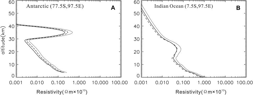
FIGURE 7. Vertical profile of atmospheric resistivity in DJF in the (A) Antarctic and (B) Indian Ocean. The solid lines are for 1990–1991, dotted lines are for 1992–1993, and dashed lines are for 1993–1994.
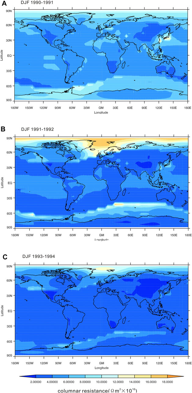
FIGURE 8. The gridded global column resistance in DJF (A) 1990–1991, (B) 1991–1992, and (C) 1993–1994.
Figure 8 shows the gridded global column resistance in DJF: 1) 1990–1991, 2) 1991–1992, and 3) 1993–1994. In panel (a), a low column resistance appears in regions with high elevations or low geomagnetic latitudes, such as East Asia, where the column resistance is controlled by surface aerosols. After the eruption of Mt. Pinatubo, due to ultrafine aerosols, the column resistance at high latitudes significantly increases, and the maximum increase could be 2.8 times. In DJF, the greatest enhancement of column resistance exists in the Northern Hemisphere. Two years after the eruption, in panel (c), the effect of ultrafine aerosols declines.
Figure 9 shows the percentage of column resistance enhancement between JJA 1993 and DJF 1993–1994. With simultaneous seasonal shifts in the column resistance, the column resistance at high latitudes undergoes large changes, and in the high latitudes of the winter hemisphere, the column resistance increases, while in the summer hemisphere, it decreases.
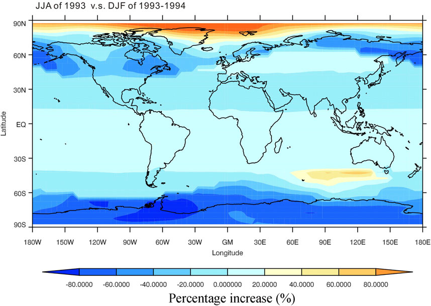
FIGURE 9. The percentage increase in column resistance between JJA 1993 and DJF 1993–1994.
Figures 10A–C show the percentage increases ((RGCR—RGCR+EEP)/RGCR)×100%, of the column resistances in DJF 1) 1990–1991, 2) 1991–1992, and 3) 1993–1994. In Figure 10A and Figure 10B, the maximum increase in the percentage of column resistance is less than 1.5%, and in Figure 10C, the maximum percentage is over 7.2% in both the northern and southern polar regions, which indicates that two years after the eruption of Mt. Pinatubo, there would be a significant effect due to the absence of EEP ionization on the column resistance. In 1990–1991 and 1991–1992, during the solar maxima, high solar activity prevented the energetic electrons from penetrating into the middle stratosphere. In 1993–1994, during the decreasing phase of solar activity, more energetic electrons reached the upper and even middle stratosphere. With ultrafine aerosols, the column resistance becomes sensitive to fluctuations in the energy particle flux.

FIGURE 10. The percentage increases ((RGCR—RGCR+EEP)/RGCR)×100%, of column resistance due to different external ionization sources in DJF (A) 1990–1991, (B) 1991–1992, and (C) 1993–1994.
Although the contribution of atmospheric resistivity from the sulfate aerosol layer in the lower stratosphere, called the Junge layer, is larger in the present simulation than in the previous TZ06 model (Tinsley et al., 2006), the aerosols in the upper stratosphere still seem to have a main effect on the column resistance at high latitudes. The ultrafine aerosol layer has a significant effect on the column resistance after the volcanic eruption. Tinsley (2005) claimed that there was an ultrafine aerosol layer in the upper stratosphere formed by ion media nucleation, as suggested by Yu and Turco(2001), which could be consistent with the unexplained variability on all time scales in measured stratospheric conductivity (Tinsley, 2005; Bering et al., 2005), especially in the descending branch of the Brewer-Dobson circulation at high latitudes. In the GEC model of the TZ06 model, the artificial ultrafine aerosol layer centered at 40 km was modeled based on the numerical simulation by Yu and Turco (2001) for an H2SO4 mass concentration of 6.35 × 10² μg m−3, which corresponds to a mass mixing ratio of 16 ppbm for the liquid droplets. In the TZ06 model, the sensitivity simulation showed that in the high volcanic eruption period, the column resistance in the high geomagnetic latitude region would be more sensitive to fluctuations in GCRs than in the low volcanic eruption period by a factor of two times due to the attribution of ultrafine aerosols and the high sensitivity of the polar region (Tinsley et al., 2006). Tinsley (2008) expected that the ultrafine aerosol concentration would have a maximum effect on the column resistance two years after a large volcanic eruption. However, in the present simulation, based on the chemical-climate model, the SAD in the ultrafine sulfate aerosol layer first appears in the descending branch of the Brewer-Dobson circulation at high latitudes soon after the eruption of Mt. Pinatubo, which significantly affects the regional column resistance. Different from previous models (TZ06, Tinsley et al., 2006), the column resistance response to volcanic eruptions shows a significant asymmetric structure in different hemispheres, and the column resistance in the high latitudes of the Northern Hemisphere has a larger response than that of the Southern Hemisphere. Two years after the volcanic eruption, the effect of ultrafine aerosols appears in only the North Atlantic region. This asymmetric structure might explain why more significant connections on day-to-day or annual time scales between space weather events and tropospheric responses, such as dynamic responses (Lam et al., 2014), cloud cover (Voiculescu et al., 2013) and cloud radiation (Frederick et al., 2019), appeared in the Northern Hemisphere than in the Southern Hemisphere.
It has been claimed that the Brewer-Dobson circulation is strengthened in the winter hemisphere (Butchart, 2014). Then, in the winter hemisphere, the transport rate of sulfate in the stratosphere is accelerated, and more ultrafine aerosols can be produced, which causes higher column resistance in the high latitude region of the winter hemisphere than in that of the summer hemisphere. In previous work, the main seasonal variation in the column resistance was mainly due to variations in the aerosol concentration in the troposphere due to changes in the boundary layer or emissions (Tinsley et al., 2006).
Many studies based on satellite observations and weather monitoring data have shown a significant connection between the fluctuations of space particles, such as GCRs, EEP, relativistic electron precipitation (REP), and the troposphere. The hypothesis suggested by Tinsley (2008) claimed that the return atmosphere current density (Jz) from the ionosphere to the land surface, which is partly controlled by atmospheric column resistance, could significantly affect the dynamic and thermal character in the troposphere through cloud electric microphysics, called the electri-scavenging or electri-anti-scavenging effect. The shorting out of the resistance of the ultrafine layer appears to be essentially when it occurs with REP, which produces bremsstrahlung X-rays that can dominate ion pair production in the middle stratosphere (Frahm et al., 1997). On the basis of SAMPEX measurements, this is likely to be most of the time at sub-auroral latitudes (Li et al., 2001a; Li et al., 2001b). However, for a few days around the times of HCS crossings, the REP decreases by up to an order of magnitude (Tinsley et al., 2000; Kirkland et al., 1996; Kniveton and Tinsley, 2004). Then, the column resistance in the sub-auroral region could increase to a high value, as calculated for the high volcanic aerosol situation, and Jz would decrease. This scenario for a decrease in Jz around the times of HCS crossings, when there is a high concentration of stratospheric aerosols, is in accordance with the sparse and noisy Jz observations for those times (Reiter, 1977; Fischer and Miihelisen, 1980; Tinsley et al., 1994). Because of the lack of a detailed model to simulate the global ion production rate due to REP, the effect of EEP is considered in the present model. The treatment of ultrafine aerosol concentrations and stratospheric ion mobility in the model confirms the essential contribution of ultrafine aerosols to column resistance. Even two years after a large volcanic eruption, the column resistance could still be sensitive to fluctuations in electron precipitation.
When the EEP effect was coupled with the seasonal effect, it could be predicted that the column resistance would be more sensitive to EEP changes in the winter hemisphere, which is consistent with most of the data analysis results.
Clouds seems to play an important role in local column resistance. The ZT09 model claimed that the variation in clouds caused less than 10% of the global atmospheric resistance, while the BTNL2013 model claimed that the effect of clouds was underestimated by the ZT09 model. Clouds are also a highly variable factor in atmospheric systems, in addition to total cloud coverage and cloud microphysics. While clouds are unstable and most cloud effects appear at low and middle latitudes, in high latitudes, ultrafine aerosols seem to be more important. Therefore, in the next step of the global circuit model, involving accurate clouds could be an important direction.
An updated global circuit model based on a chemistry-climate model (SOCOL-AERv2) with an accurate aerosol formation process is set up. The results provide a more accurate evaluation of the layer of ultrafine aerosols on global column resistance. The asymmetric distribution of ultrafine aerosols causes different responses of local column resistance to fluctuations in energetic particle precipitation. Column resistance in the high latitudes of the winter hemisphere would be more sensitive to energetic particle precipitation than that of the summer hemisphere. Since the EEP flux could contribute more relativistic electrons in the middle stratosphere, with the apparent ultrafine aerosol layer, the column resistance in the winter hemisphere would be more sensitive to fluctuations in the flux of REP. The whole atmosphere chemistry-climate model coupled with the global circuit sub-model including accurate ion pair production by REP could provide a clearer picture of the link between space weather and the troposphere.
The raw data supporting the conclusion of this article will be made available by the authors, without undue reservation.
LZ, designing the work for the publication and making the original GEC model, taking in charge of the whole work; YX, operating the updated global circuit model and finishing 80% writing work for the manuscript; RZ, operating the SOCOL_AER model and finishing 20% writing work of the manuscript; ZZ, operating the SOCOL_AER model.
This work was funded in part by the Strategic Priority Research Program of CAS (Grant No. XBD 41000000) and the National Science Foundation of China (41971020, 41905059).
The authors declare that the research was conducted in the absence of any commercial or financial relationships that could be construed as a potential conflict of interest.
Bates, D. R. (1982). Recombination of Small Ions in the Troposphere and Lower Stratosphere. Planet. Space Sci. 30 (12), 1275–1282. doi:10.1016/0032-0633(82)90101-5
Baumgaertner, G. A. J., Thayer, J. P., Neely, R. R., and Lucas, G. (2013). Toward a Comprehensive Global Electric Circuit Model: Atmospheric Conductivity and its Variability in CESM1(WACCM) Model simulations. J. Geophys. Res. Atmos. 118 (16), 9221–9232. doi:10.1002/jgrd.50725
Bering, E. A., Benbrook, J. R., Holzworth, R. H., Byrne, G. J., and Gupta, S. P. (2005). Latitude Gradients in the Natural Variance in Stratospheric Conductivity Implications for Studies of Long-Term Changes. Adv. Space Res. 35 (8), 1385–1397. doi:10.1016/j.asr.2005.04.017
Bering, E. A., Few, A. A., and Benbrook, J. R. (1998). The Global Electric Circuit. Phys. Today 51 (10), 24–30. doi:10.1063/1.882422
Butchart, N. (2014). The Brewer‐Dobson Circulation. Rev. Geophys. 52 (2), 157–184. doi:10.1002/2013rg000448
Egorova, T. A., Rozanov, E. V., Zubov, V. A., and Karol, I. L. (2003). Model for Investigating Ozone Trends (MEZON). Izvestiya Atmos. Oceanic Phys. 39 (3), 277–292.
Egorova, T., Rozanov, E., Ozolin, Y., Shapiro, A., Calisto, M., Peter, T., et al. (2011). The Atmospheric Effects of October 2003 Solar Proton Event Simulated with the Chemistry-Climate Model SOCOL Using Complete and Parameterized Ion Chemistry. J. Atmos. Solar-Terrestrial Phys. 73 (2), 356–365. doi:10.1016/j.jastp.2010.01.009
English, J. M., Toon, O. B., Mills, M. J., and Yu, F. (2011). Microphysical Simulations of New Particle Formation in the Upper Troposphere and Lower Stratosphere. Atmos. Chem. Phys. 11 (17), 9303–9322. doi:10.5194/acp-11-9303-2011
Fang, X., Randall, C. E., Lummerzheim, D., Wang, W., Lu, G., Solomon, S. C., et al. (2010). Parameterization of Monoenergetic Electron Impact Ionization. Geophys. Res. Lett. 37 (22), 1–5. doi:10.1029/2010gl045406
Feinberg, A., Sukhodolov, T., Luo, B.-P., Rozanov, E., Winkel, L. H. E., Peter, T., et al. (2019). Improved Tropospheric and Stratospheric Sulfur Cycle in the Aerosol-Chemistry-Climate Model SOCOL-AERv2. Geosci. Model. Dev. 12 (9), 3863–3887. doi:10.5194/gmd-12-3863-2019
Fischer, H. J., and Mühleisen, J. (1980). The Ionospheric Potential and the Solar Magnetic Sector Boundary Crossings. Rep. Astron. Inst., Univ. Tübingen, Ravensburg, Germany.
Frahm, R. A., Winningham, J. D., Sharber, J. R., Link, R., Crowley, G., Gaines, E. E., et al. (1997). The Diffuse aurora: A Significant Source of Ionization in the Middle Atmosphere. J. Geophys. Res. 102 (D23), 28203–28214. doi:10.1029/97jd02430
Frederick, J. E., Tinsley, B. A., and Zhou, L. (2019). Relationships between the Solar Wind Magnetic Field and Ground-Level Longwave Irradiance at High Northern Latitudes. J. Atmos. Solar-Terrestrial Phys. 193, 105063. doi:10.1016/j.jastp.2019.105063
Funke, B., López-Puertas, M., Stiller, G. P., Versick, S., and von Clarmann, T. (2016). A Semi-empirical Model for Mesospheric and Stratospheric NOy Produced by Energetic Particle Precipitation. Atmos. Chem. Phys. 16 (13), 8667–8693. doi:10.5194/acp-16-8667-2016
Hays, P. B., and Roble, R. G. (1979). A Quasi-Static Model of Global Atmospheric Electricity, 1. The Lower Atmosphere. J. Geophys. Res. 84 (A7), 3291–3305. doi:10.1029/ja084ia07p03291
Hebert, L., Tinsley, B. A., and Zhou, L. (2012). Global Electric Circuit Modulation of winter Cyclone Vorticity in the Northern High Latitudes. Adv. Space Res. 50 (6), 806–818. doi:10.1016/j.asr.2012.03.002
Hess, M., Koepke, P., and Schult, I. (1998). Optical Properties of Aerosols and Clouds: The Software Package OPAC. Bull. Amer. Meteorol. Soc. 79 (5), 831–844. doi:10.1175/1520-0477(1998)079<0831:opoaac>2.0.co;2
Holzworth, R. H., Norville, K. W., and Williamson, P. R. (1987). Solar Flare Perturbations in Stratospheric Current Systems. Geophys. Res. Lett. 14 (8), 852–855. doi:10.1029/gl014i008p00852
Höpfner, M., Glatthor, N., Grabowski, U., Kellmann, S., Kiefer, M., Linden, A., et al. (2013). Sulfur Dioxide (SO2) as Observed by MIPAS/Envisat: Temporal Development and Spatial Distribution at 15-45 Km Altitude. Atmos. Chem. Phys. 13 (20), 10405–10423. doi:10.5194/acp-13-10405-2013
Hoppel, W. A. (1985). Ion-Aerosol Attachment Coefficients, Ion Depletion, and the Charge Distribution on Aerosols. J. Geophys. Res.. 90 (D4), 5917–5923. doi:10.1029/JD090iD04p05917
Junge, C. E., and Manson, J. E. (1961). Stratospheric Aerosol Studies. J. Geophys. Res. 66 (7), 2163–2182. doi:10.1029/jz066i007p02163
Kirkland, M. W., Tinsley, B. A., and Hoeksema, J. T. (1996). Are Stratospheric Aerosols the Missing Link Between Tropospheric Vorticity and Earth Transits of the Heliospheric Current Sheet?. J. Geophy. Res.: Atmosphe. 101 (D23), 29689–29699. doi:10.1029/96JD01554
Kniveton, D. R., and Tinsley, B. A. (2004). Daily changes in global cloud cover and Earth transits of the heliospheric current sheet. J. Geophys. Res. 109, D11201. doi:10.1029/2003JD004232
Kniveton, D. R., Tinsley, B. A., Burns, G. B., Bering, E. A., and Troshichev, O. A. (2008). Variations in Global Cloud Cover and the Fair-Weather Vertical Electric Field. J. Atmos. Solar-Terrestrial Phys. 70 (13), 1633–1642. doi:10.1016/j.jastp.2008.07.001
Lam, M. M., Chisham, G., and Freeman, M. P. (2014). Solar Wind-Driven Geopotential Height Anomalies Originate in the Antarctic Lower Troposphere. Geophys. Res. Lett. 41 (18), 6509–6514. doi:10.1002/2014gl061421
Lam, M. M., and Tinsley, B. A. (2016). Solar Wind-Atmospheric Electricity-Cloud Microphysics Connections to Weather and Climate. J. Atmos. Solar-Terrestrial Phys. 149, 277–290. doi:10.1016/j.jastp.2015.10.019
Li, X., Baker, D. N., Kanekal, S. G., Looper, M., and Temerin, M. (2001a). Long Term Measurements of Radiation Belts by SAMPEX and Their Variations. Geophys. Res. Lett. 28 (20), 3827–3830. doi:10.1029/2001gl013586
Li, X., Temerin, M., Baker, D. N., Reeves, G. D., and Larson, D. (2001b). Quantitative Prediction of Radiation belt Electrons at Geostationary Orbit Based on Solar Wind Measurements. Geophys. Res. Lett. 28 (9), 1887–1890. doi:10.1029/2000gl012681
Lin, S.-J., and Rood, R. B. (1996). Multidimensional Flux-form Semi-lagrangian Transport Schemes. Mon. Wea. Rev. 124 (9), 2046–2070. doi:10.1175/1520-0493(1996)124<2046:mffslt>2.0.co;2
Lucas, G. M., Baumgaertner, A. J. G., and Thayer, J. P. (2015). A Global Electric Circuit Model within a Community Climate Model. J. Geophys. Res. Atmos. 120 (23), 12054–12066. doi:10.1002/2015jd023562
Makino, M., and Ogawa, T. (1985). Quantitative Estimation of Global Circuit. J. Geophys. Res. 90 (D4), 5961–5966. doi:10.1029/jd090id04p05961
Mironova, I., Karagodin-Doyennel, A., and Rozanov, E. (2021). The Effect of Forbush Decreases on the Polar-Night HOx Concentration Affecting Stratospheric Ozone. Front. Earth Sci. 8, 669. doi:10.3389/feart.2020.618583
Mlawer, E. J., Taubman, S. J., Brown, P. D., Iacono, M. J., and Clough, S. A. (1997). Radiative Transfer for Inhomogeneous Atmospheres: RRTM, a Validated Correlated-K Model for the Longwave. J. Geophys. Res. 102 (D14), 16663–16682. doi:10.1029/97jd00237
Morcrette, J. (1991). Evaluation of Model-generated Cloudiness: Satellite-observed and Model-generated Diurnal Variability of Brightness Temperature. Monthly Weather Rev. 119 (5), 1205–1224. doi:10.1175/1520-0493(1991)119<1205:EOMGCS>2.0.CO;2
Reiter, R. (1997). The Electric Potential of the Ionosphere as Controlled by the Solar Magnetic Sector Structure. Result of a Study Over the Period of a Solar Cycle. J. Atmosph. Terrestrial Phys. 39 (1), 95–99.
Rinsland, C. P., Gunson, M. R., Ko, M. K. W., Weisenstein, D. W., Zander, R., Abrams, M. C., et al. (1995). H2SO4photolysis: A Source of Sulfur Dioxide in the Upper Stratosphere. Geophys. Res. Lett. 22 (9), 1109–1112. doi:10.1029/95GL00917
Roeckner, E. (1995). Parameterization of clouds and radiation in climate models. United States. doi:10.2172/232602
Roeckner, E., Bäuml, G., Bonaventura, L., Brokopf, R., Esch, M., Giorgetta, M., et al. (2003). The Atmospheric General Circulation Model ECHAM 5. PART I: Model Description. Tech. Rep. 349 (Hamburg: Max-Planck-Institut für Meteorologie). Available at: http://www.mpimet.mpg.de/fileadmin/publikationen/Reports/max_scirep_349.pdf (Access July 9, 2019).
Rozanov, E. V., Zubov, V. A., Schlesinger, M. E., Yang, F., and Andronova, N. G. (1999). The UIUC Three-Dimensional Stratospheric Chemical Transport Model: Description and Evaluation of the Simulated Source Gases and Ozone. J. Geophys. Res. 104 (D9), 11755–11781. doi:10.1029/1999jd900138
Sapkota, B. K., and Varshneya, N. C. (1990). On the Global Atmospheric Electrical Circuit. J. Atmos. Terrestrial Phys. 52 (1), 1–20. doi:10.1016/0021-9169(90)90110-9
Sheng, J.-X., Weisenstein, D. K., Luo, B.-P., Rozanov, E., Stenke, A., Anet, J., et al. (2015). Global Atmospheric Sulfur Budget under Volcanically Quiescent Conditions: Aerosol-Chemistry-Climate Model Predictions and Validation. J. Geophys. Res. Atmos. 120 (1), 256–276. doi:10.1002/2014jd021985
Stenke, A., Schraner, M., Rozanov, E., Egorova, T., Luo, B., and Peter, T. (2013). The SOCOL Version 3.0 Chemistry-Climate Model: Description, Evaluation, and Implications from an Advanced Transport Algorithm. Geosci. Model. Dev. 6 (5), 1407–1427. doi:10.5194/gmd-6-1407-2013
Sukhodolov, T., Sheng, J.-X., Feinberg, A., Luo, B.-P., Peter, T., Revell, L., et al. (2018). Stratospheric Aerosol Evolution after Pinatubo Simulated with a Coupled Size-Resolved Aerosol-Chemistry-Climate Model, SOCOL-AERv1.0. Geosci. Model. Dev. 11 (7), 2633–2647. doi:10.5194/gmd-11-2633-2018
Tinsley, B. A. (1996). Correlations of Atmospheric Dynamics with Solar Wind-Induced Changes of Air-Earth Current Density into Cloud Tops. J. Geophys. Res. 101 (D23), 29701–29714. doi:10.1029/96jd01990
Tinsley, B. A., and Deen, G. W. (1991). Apparent Tropospheric Response to MeV-GeV Particle Flux Variations: A Connection via Electrofreezing of Supercooled Water in High-Level Clouds?. J. Geophys. Res. 96 (D12), 22283–22296. doi:10.1029/91jd02473
Tinsley, B. A. (2005). On the Variability of the Stratospheric Column Resistance in the Global Electric Circuit. Atmosphe. Res. 76 (1-4), 78–94. doi:10.1016/j.atmosres.2004.11.013
Tinsley, B. A. (2008). The Global Atmospheric Electric Circuit and its Effects on Cloud Microphysics. Rep. Prog. Phys. 71 (6), 066801. doi:10.1088/0034-4885/71/6/066801
Tinsley, B. A., Hoeksema, J. T., and Baker, D. N. (1994). Stratospheric Volcanic Aerosols and Changes in Air-Earth Current Density at Solar Wind Magnetic Sector Boundaries as Conditions for the Wilcox Tropospheric Vorticity Effect. J. Geophys. Res. 99 (D8), 16805–16813. doi:10.1029/94JD01207
Tinsley, B. A., and Yu, F. (2004). Atmospheric Ionization and Clouds as Links between Solar Activity and Climate. Solar Variability Its Effects Clim., Geophys. Monogr. Ser. 141, 321–339. doi:10.1029/141gm22
Tinsley, B. A., Zhou, L., and Plemmons, A. (2006). Changes in Scavenging of Particles by Droplets Due to Weak Electrification in Clouds. Atmos. Res. 79 (3-4), 266–295. doi:10.1016/j.atmosres.2005.06.004
Usoskin, I. G., Kovaltsov, G. A., and Mironova, I. A. (2010). Cosmic ray Induced Ionization Model CRAC:CRII: An Extension to the Upper Atmosphere. J. Geophys. Res. 115 (D10), 302. doi:10.1029/2009jd013142
Veretenenko, S. V., and Pudovkin, M. I. (1997). Effects of the Galactic Cosmic ray Variations on the Solar Radiation Input in the Lower Atmosphere. J. Atmos. Solar-Terrestrial Phys. 59 (14), 1739–1746. doi:10.1016/s1364-6826(96)00183-6
Voiculescu, M., Usoskin, I., and Condurache-Bota, S. (2013). Clouds Blown by the Solar Wind. Environ. Res. Lett. 8 (4), 045032. doi:10.1088/1748-9326/8/4/045032
Wilcox, J. M., Scherrer, P. H., Svalgaard, L., Roberts, W. O., and Olson, R. H. (1973). Solar Magnetic Sector Structure: Relation to Circulation of the Earth's Atmosphere. Science (New York, N.Y.) 180 (4082), 185–186. doi:10.1126/science.180.4082.185
Yu, F., and Turco, R. P. (2001). From Molecular Clusters to Nanoparticles: Role of Ambient Ionization in Tropospheric Aerosol Formation. J. Geophys. Res. 106 (D5), 4797–4814. doi:10.1029/2000jd900539
Zhou, L., and Tinsley, B. A. (2010). Global Circuit Model with Clouds. J. Atmos. Sci. 67 (4), 1143–1156. doi:10.1175/2009jas3208.1
Zhou, L., Tinsley, B., and Huang, J. (2014). Effects on winter Circulation of Short and Long Term Solar Wind Changes. Adv. Space Res. 54 (12), 2478–2490. doi:10.1016/j.asr.2013.09.017
Keywords: global electric circuit, ultrafine aerosol, column resistance, brewer-dobson circulation, solar activity
Citation: Xie Y, Zhang R, Zhu Z and Zhou L (2021) Evaluating the Response of Global Column Resistance to a Large Volcanic Eruption by an Aerosol-Coupled Chemistry Climate Model. Front. Earth Sci. 9:673808. doi: 10.3389/feart.2021.673808
Received: 28 February 2021; Accepted: 04 May 2021;
Published: 16 June 2021.
Edited by:
Irina Alexandrovna Mironova, Saint Petersburg State University, RussiaReviewed by:
Arseniy Karagodin-Doyennel, Physikalisch-Meteorologisches Observatorium Davos, SwitzerlandCopyright © 2021 Xie, Zhang, Zhu and Zhou. This is an open-access article distributed under the terms of the Creative Commons Attribution License (CC BY). The use, distribution or reproduction in other forums is permitted, provided the original author(s) and the copyright owner(s) are credited and that the original publication in this journal is cited, in accordance with accepted academic practice. No use, distribution or reproduction is permitted which does not comply with these terms.
*Correspondence: Limin Zhou, bG16aG91QGdlby5lY251LmVkdS5jbg==
Disclaimer: All claims expressed in this article are solely those of the authors and do not necessarily represent those of their affiliated organizations, or those of the publisher, the editors and the reviewers. Any product that may be evaluated in this article or claim that may be made by its manufacturer is not guaranteed or endorsed by the publisher.
Research integrity at Frontiers
Learn more about the work of our research integrity team to safeguard the quality of each article we publish.