West Pacific Earthquake Forecasting Using NOAA Electron Bursts With Independent L-Shells and Ground-Based Magnetic Correlations

Recent advances in statistical correlations between strong earthquakes and several non-seismic phenomena have opened the possibility of formulating warnings within days or even hours. The retrieved correlations have been discovered for those ionospheric physical observations which lasted a long time and realized using the same instruments, including multi-satellite recordings. One of those regarded the electron burst phenomena detected by NOAA, for which the conditional probability of a seismic event was calculated. Then an earthquake probability greater than its frequency was assigned when a satellite realized such a phenomenological observation. This approach refers to the correlations obtained between high-energy electrons detected using the NOAA POES and strong Indonesian and Philippine earthquakes. It is reformulated here to realize a test of earthquake forecasting. The fundamental step is obtained by using a unique electron L-shell interval of $1.21\le L\le 1.31$, which decouples the electron parameters from the earthquake parameters. Then, the optimized correlation was recalculated to be 1.5–3.5 h early, between electron bursts and an increased number of seismic events with $M\ge 6$, therein improving the significance too. Moreover, this methodology is reconnected to the frequency theory, and to Molchan’s error diagram, by the probability gain, where a comparison among the significances of various methods is given. The previously proposed physical link between the crust and the ionosphere through magnetic interaction, presumably operating 4–6 h before strong earthquakes, is examined quantitatively on the basis of recent magnetic pulse measurements. Consequently, the probability gain of earthquake forecasting is hypothetically calculated for both the dependent measurements of electron bursts using NOAA satellites and possible ground-based magnetic pulse detection. This method of combining probability gains for earthquake forecasting is general enough that it can be applied to any pair of observables from space and the ground.

Introduction

Different phenomena, possibly connected with seismic activity, have been reported in recent years by many authors researching anomalies, both geoscientific (Rikitake, 1976; Rikitake, 1987) and macroscopic (Rikitake, 2003). Their research has reported instrumentally repeated observations occurring with strong earthquakes (EQs), and this has permitted them to identify important statistical behavior (Rikitake, 2003). However, in the absence of a recording network, almost all the results are dependent on individual properties of recording, and this renders it rather difficult to obtain an estimation on reasonable statistics (Molchanov and Hayakawa, 2008). The limited number of observatories on the ground and their punctual observations, even when operative (Console, 2001), reduce the number of considered strong EQs, making it too small to calculate a statistical correlation over several decades. Only when moderate magnitude EQs are considered, a statistical correlation is currently calculated for ULF geomagnetic fluctuations at ground stations (Schekotov et al., 2006; Hattori et al., 2013; Han et al., 2014; Han et al., 2017). In other studies, Pc1 anticipated EQs by 6–7 days (Bortnik et al., 2008), VLF noise by 2 days (Oike and Yamada, 1994), lightning activities 17–19 days before EQs (Liu et al., 2015), and geoelectric fields with lead times from days to weeks (An et al., 2020). A review of several correlation increases corresponding to 3 days between ELF Q-bursts and the Kanchakta EQs has been reported with the possible associated physical models (Hayakawa et al., 2019). A method to predict the time, epicenter, and magnitude of such events has been suggested (Schekotov et al., 2019) based on the works cited above.

Observations made by low-orbit satellites are able to monitor large portions of the ground in a few hours, allowing the monitoring of the area affected by each seismic event (Barnhart et al., 2019), and to consider all, or a large portion, of strong EQs. Satellite detection techniques and communication developments are made using electromagnetic instruments and have therefore been immediately used to monitor electromagnetic fields in the ionosphere. Electromagnetic fields measured in the low Earth orbits were associated with strong EQ occurrence for the first time in the 1980s, with regard to electric and magnetic intensity in the range of 1 Hz–10 kHz, when satellites arrived close to EQ epicentres (Larkina et al., 1983; Parrot and Lefeuvre, 1985; Larkina et al., 1989; Parrot and Mogilevsky, 1989; Mikhaylova et al., 1991; Serebryakova et al., 1992). A space-borne system for short-term EQ warning has been suggested (Pulinets, 1998a; Parrot, 2002; Pulinets, 2006), and as ionospheric perturbations measured using satellites are not only due to EQs and are not found for all EQs, a statistical analysis of a possible influence of the seismic activity on the ionosphere is preferred (Parrot, 2011). Statistical results were obtained in 1993 using the Intercosmos-24 satellite (Molchanov, 1993), where the probability of charged particle burst observations was from 6 to 24 h before the event increased by 50%, and the DE-2 satellite (Henderson et al., 1993), where no significant differences occurred between EQ orbits and control orbits. Moreover, the average wave intensity received on board the AUREOL-3 satellite (Parrot, 1994) increased with seismic activity, resulting in an extension in the latitude direction but not in the longitude, with respect to EQ epicentres. The ISIS 1 and 2 satellites have been used to identify the spectra of electromagnetic radiation of seismic events under control data (Rodger et al., 1996), showing no significant evidence for differences between data sets of the EQs and control orbits. A statistical study of intensity for VLF electromagnetic waves has been realized in the vicinity of EQ epicentres using the micro-satellite DEMETER (Nemec et al., 2008). It has evidenced a significant decrease in the measured wave intensity, 0–4 h before strong EQs. A confirmation of this result, on a longer set of data, was obtained (Nemec et al., 2009), suggesting that a significant decrease is occurring for larger EQs, is stronger for shallower EQs, and does not seem to depend on whether the EQ occurs below an ocean or not.

Anomalies appearing in electron densities of the ionospheric F-region a few days before strong EQs were observed (Pulinets 1998b; Liu et al., 2000; Pulinets and Boyarchuk, 2004; Liu et al., 2006). These anomalies concern the electron densities recorded using local ionosondes, where the critical frequency of the F2-peak, foF2, significantly decreased days before several EQs. Moreover, decreasing electron densities, days before strong EQs in Taiwan, had been compared with the total electron content (TEC) calculated using ground-based GPS receivers and satellite transmitters (Liu et al., 2004). Anomalous TEC signals were observed in Southern California, but no statistically significant correlations regarding time and space between these TEC anomalies and the occurrence of seismic events resulted (Thomas et al., 2007). On the other hand, positive results for the correlation of EQ from 2 to 5 days after TEC fluctuations have been obtained (Li and Parrot, 2013). Study results from Taiwan support the result that the equatorial ionization anomaly crest significantly moves equatorward 1–5 days before strong EQs (Liu et al., 2010). A statistical analysis carried out on TEC data from the global ionosphere map evidenced that the largest occurrence rates of anomalies were for those EQs with larger magnitudes and lower depths 1–5 days before the EQs (Liu et al., 2011; Zhu et al., 2014). This was confirmed by Japanese (Kon et al., 2011) and Chinese (Ke et al., 2016) studies. Vertical TEC positive and negative anomalies aligned parallel with the local geomagnetic field were repeatedly observed 20–40 min before three $M>8$ Chilean EQs (He and Heki, 2016). Concentrations of electron density and magnetic anomalies for more than two months to some days before the EQ occurrences have been reported worldwide (De Santis et al., 2019). However, a 14-year analysis of data did not reveal any statistically significant changes prior to EQs when considering all of the 1,279 EQs together (Thomas et al., 2017). Using GPS TEC measurements, a statistical analysis and comparison of the temporal and spatial distributions for the pre-EQ ionospheric anomalies before the $1\text{,}339M\ge 6.0\text{ EQs}$, which occurred globally between January 2003 and December 2014, did not provide reliable evidence of pre-EQ changes on the global ionospheric map of TEC data (Zhu et al., 2018).

Ionospheric perturbations with seismic activity have included wave paths of VLF and LF transmitters (Molchanov and Hayakawa, 1998; Biagi et al., 2001). The VLF and LF amplitude observations are connected with the entire path covered by waves, even if they are obtained in a punctual station, thus representing an intermediate type of observation between the purely punctual and the completely diffused realized using satellites. Seismo-ionospheric effects on long sub-ionospheric paths have been investigated in amplitude variations of signals and have used the VLF terminator time method (Clilverd et al., 1999), indicating that the occurrence rate of successful EQ predictions using it cannot be distinguished with respect to a random one. Statistical results obtained by the superimposed epoch analysis in Japan (Maekawa et al., 2006) yielded that the ionosphere was definitively disturbed in terms of both amplitude and dispersion. For an integrated energy, released within the interested area for the LF wave path, the amplitude is depleted and the dispersion is very much enhanced for about one week to a few days before the EQ. A statistical correlation between EQs and VLF/LF signals over 10 years or so, obtained by means of the Japanese VLF/LF network, revealed perturbations 3–6 days prior to wave paths (Hayakawa et al., 2010).

A correlation analysis between earthquakes and atmospheric temperature variations over several months observed using a portable meteostation obtained a time anticipation of about one day (Molchanov et al., 2003). Consequently, thermal infrared anomalies have also been observed with strong EQs from space. A complete review has reported the main contributions and results achieved over 30 years (Tramutoli et al., 2015). Molchan’s error diagram analysis computed for different classes of magnitude and significant sequences of thermal infrared anomalies has suggested a prognostic probability gain when compared to random guess results, both for strong EQs in Greece (Eleftheriou et al., 2016) and in the Sichuan area (Zhang and Meng, 2019).

Sudden variations in high-energy charged particle fluxes near the South Atlantic Anomaly have also been associated with seismic activity (Voronov et al., 1989). In fact, numerous experiments followed the discovery of the Van Allen Belts (Van Allen, 1959) to determine safe conditions for near-Earth space exploration. Further detection of charged particle flux variations associated with strong EQs was obtained using the Intercosmos-24 satellite (Galperin et al., 1992; Boskova et al., 1994), resulting in precipitating particles which escaped the trapped conditions of the geomagnetic field. High-energy precipitating particle fluxes have been statistically analyzed in relation to seismic activity in various near-Earth space experiments such as the MIR orbital station and the METEOR-3, GAMMA, and SAMPEX satellites, which have shown particle bursts 2–5 h before EQs (Aleksandrin et al., 2003). A reanalysis of the more recent and extended SAMPEX database has also shown a 3–4 h correlation with precipitating high-energy electrons anticipating strong EQs (Sgrigna et al., 2005). The NOAA-15 satellite particle database, which has been collecting data since 1998, has been systematically studied (Fidani et al., 2010). Sudden variations in high-energy charged particles have been connected with strong EQs in periods of weak solar activity (Fidani, 2015). This statistical correlation analysis evidenced that exceptional increases in electron fluxes occurring 2–3 h prior to the largest quakes had struck the Indonesian and Philippine investigated areas between 1998 and 2014. The correlated EQs occurred at a depth less than 200 km, independent of sea or land. Precipitating particles have been detected far from EQ geographical positions, so the possible disturbances above the EQ epicenters due to particle drift have been estimated to be in the range of 4–6.5 h before strong seismic events (Fidani, 2018).

Definitely, several studies’ results have suggested that ionospheric phenomena appear to statistically precede strong earthquakes by up to a week, and some studies even propose longer anticipation times. However, the demonstration of the physical link between the two phenomena is essential to affirm that one of the two is more than a candidate precursor for the other. Moreover, short-term EQ precursors are thought to precede by 1–2 days to several weeks, and near-seismic precursors are thought to precede by several hours to 1–2 days (Molchanov and Hayakawa, 2008). Therefore, electromagnetic fluctuations detected using satellites both in the ELF and VLF bands, together with particle precipitation, may belong to the class of near-seismic candidate precursors, whereas TEC, together with both VLF and LF path amplitude depletion, and geoelectric ULF fields may belong to the class of short-term candidate precursors. As for ground observations, VLF noise belongs to the class of near-seismic candidate precursors, and Pc1 pulsations and lightning activity may belong to the class of short-term candidate precursors, while ELF Q-bursts, Schumann resonances, and ULF magnetic depressions may belong to both classes. The recent results on EQ observations, carried out using low Earth orbit satellites, can be found in a publication by Ouzounov et al. (2018).

Given the possibility reported above to observe physical phenomena that recurrently, and with statistical significance, anticipate strong EQs, a verification of EQ forecasting has been formulated on the basis of schemes already used, starting from the statistical study of seismicity (Console, 2001). In particular, the previously calculated correlations between NOAA electron precipitations and EQs are examined in the fundamental steps, showing what remains ambiguous for electron identification, in Reviewing NOAA Electrons’ Statistical Correlations. A reproduction of the statistical correlation between completely decoupled NOAA electron precipitations and EQs, so as to define the precursor phenomenon unambiguously (Wyss, 1997), is obtained in Unambiguous NOAA Electrons’ Statistical Correlation. NOAA correlations are reviewed using classic statistical frequency techniques, and their statistical significance is calculated using recent methods of error diagrams in Forecasting Methodologies and Evaluating Significance, where a complete equivalence among these approaches is demonstrated. The objective is to define a methodology to introduce one or more statistically verified precursors in EQ forecasting using conditional probabilities. Prediction Model is devoted to building a prediction scenario following the work of Console (2001). A discussion of any possible relevance to the improvement of the probability gain derived from dependent precursors used together, observed both on the Earth’s surface and from space, is presented in Dependent Observables. Finally, the electron precipitations’ possible dependence on magnetic pulses is shown using a physical model in Different Precursors Combined, and a hypothetical experiment demonstrates the probability gain due to these two dependent observations. The conclusion is reported in Conclusion with a sequence of steps that combine interdependent observations for EQ forecasting.

Materials and Methods

To systematically test methodologies of precursors, for which a statistical analysis of past cases is feasible, the conditional probability of occurrence (Aki, 1981) is a desirable parameter that should supplement the usual time–location–magnitude parameters of the prediction (Console, 2001). Several physical observations on the Earth’s surface and from space have been successfully correlated with EQs. However, a conditional probability has only been obtained from the analysis of the NOAA satellites’ precipitating electrons (Fidani, 2018; Fidani, 2019; Fidani, 2020), so it would be the most suitable methodology to be tested.

Reviewing NOAA Electrons’ Statistical Correlations

NOAA polar satellites use particle detectors which monitor fluxes of protons and electrons in polar orbits at altitudes between 807 and 854 km (Davis, 2007). The particle detectors (Space Environment Monitor SEM-2) consist of the total energy detector (TED) and the medium energy proton and electron detector (MEPED). The MEPED is composed of eight solid-state detectors measuring proton and electron fluxes from 30 keV to 200 MeV (Evans and Greer, 2004) which include the radiation belt populations, energetic solar particle events, and the low-energy portion of the galactic cosmic ray population. Data can be downloaded at the link http://www.ngdc.noaa.gov/stp/satellite/poes/dataaccess.html. As all of the sets of orbital parameters are provided every 8 s, this value was chosen as the basic time step for our study (Fidani and Battiston, 2008). Consequently, all other variables were defined with respect to the 8-s step. Thus, 8-s averages of the counting rates (CRs), latitude, longitude, MEPED, and omnidirectional data were calculated. Unreliable CRs with negative values were labeled and excluded from the analysis.

To systematically test the methodology proposed for NOAA data, a quantitative and rigorous definition of the concerned precursor (Console, 2001) was established. The daily averages of particle CRs exiting the entrapment in the geomagnetic field (precipitations) were calculated, and then the condition for which a CR fluctuation was not likely, due to possible statistical fluctuations, was set. This calculation was formulated with a probability larger than 99% (Fidani et al., 2010). The sudden increase in particle flux that satisfies this condition was named particle burst (Sgrigna et al., 2005), and for electrons, the same condition was named electron burst (EB). According to a previous work (Aleksandrin et al., 2003), the daily averages of CRs were calculated in the invariant coordinate space. Together with the L-shell and the pitch angle, it was necessary to take into account the CR amplitudes and their variations versus geomagnetic coordinates, since the spatial gradient of particle fluxes near the South Atlantic Anomaly (SAA) is too large (Fidani and Battiston, 2008). CR distributions inside invariant areas are compatible with a Poisson distribution. Being so, an amplitude threshold was introduced for the CRs to define the conditions for which a CR is a non-Poissonian fluctuation with 99% probability. Furthermore, NOAA satellites measure variations of ionospheric parameters not only due to EQs; indeed, they are principally due to solar activity (Sgrigna et al., 2005; Parrot, 2011). To reduce the effects of solar activity, both low values in Dst variations (http://wdc.kugi.kyoto-u.ac.jp/dst_final/index.html) and geomagnetic Ap indexes (https://www.ngdc.noaa.gov/geomag/data.shtml) were chosen to exclude CR data corresponding to the Sun’s influence (Fidani, 2015).

To conclude the quantification of the precursor (Console, 2001), the L-shell invariant parameter was considered to define the magnetic line where a physical interaction, whatever it is, can connect the seismic and ionospheric activities. Following the works by Aleksandrin et al. (2003) and Sgrigna et al. (2005), particle bursts were considered only when their L-shell values referred to $M\mathrm{\ge }6$ EQ epicenter projections that occurred on the magnetic lines. This is equivalent to imagining that the physical interaction can occur in the same region near the vertical. The correlation was calculated by filling a histogram with the time differences $\Delta t$ between the EQs and EBs, which was indicated by ${\displaystyle {\sum }_{\{EQ;EB\}}\left(EQ\times EB\right)}$ following the work of Fidani (2015). This approach was performed by considering only EB on magnetic lines identified as projecting EQ coordinates at different altitudes with respect to EQ epicenters, from −600 km up to 3,200 km in increments of 100 km. A correlation peak at $\Delta t=2-3\text{h}$ started to be significant only for 30–100-keV EBs when considering magnetic line altitudes above 1,400 km and was maximized for 2,200 km (Fidani, 2015) (see Figure 1). Correlations were maximized by using EQs with magnitudes $M\ge 6$ downloaded at the link https://earthquake.usgs.gov/earthquakes/search/, located in both the Indonesian and the Philippine regions, having 90°–150° longitudes, with few events in South America. The EBs were detected high off the shore of the United States and the west coasts of South America, at longitudes between 200° and 280°. These different electron positions were associated in a causal way, due to the fact that electrons drift eastward and the EQ positions were located west of the EB detection positions (Fidani, 2018; Fidani, 2020). Being so, if the disturbances which caused electron precipitations from inner radiation belts occurred above the EQ epicenters in the ionosphere, they most likely anticipated the EQ times by 4–6.5 h.

FIGURE 1

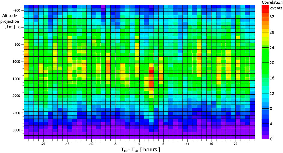
FIGURE 1. Complete correlation histogram between EBs and EQs obtained between −24 and 24 h and projecting the EQ epicenters between −600 and 3,200 km. The correlation event palette on the right provides the number of EQs that contributed to the correlation. A positive $\Delta t=T_{EQ}-T_{EB}$ means that the time of an EQ is greater than the time of an EB, highlighting that the EB anticipated the EQ.

However, to consider EB L-shells around the L-shells corresponding to the EQ epicenter projected at several altitudes constitutes an ambiguity in defining the phenomena that preceded EQs. In fact, the L-shell parameter to choose EB involves both EB and EQ events and each EQ event with a multiplicity of altitude projections. So, the request for the L-shell parameter, which is only related to EBs, is lost and EB cannot be chosen unambiguously. Furthermore, if the condition of L-shell similarity between considered EB detection and EQ projections is not satisfied, the correlation cannot be found. In conclusion, the steps used to calculate any statistical correlation between EBs and EQs are ambiguous, so they cannot be used to define a phenomenon that anticipates strong EQs. In particular, the step involving the L-shell of EBs needs to be modified for the EQ forecasting.

Unambiguous NOAA Electrons’ Statistical Correlation

The NOAA-15 MEPED telescope used to monitor the electron flux coming from the zenith in three energy bands in the range of 30 keV–2.5 MeV (Evans and Greer, 2004) has been used. The energy detected for the electrons is a cumulative sum over three thresholds: $E_1=30\text{keV}$, $E_2=100\text{keV}$, and $E_3=300\text{keV}$. Since different energies determine different behaviors in particle dynamics, new energy channels were derived from the difference of the energy thresholds to obtain electrons detected in the intervals 30–100 keV, 100–300 keV, and 300–2.5 MeV. CRs were then corrected for proton contamination (Rodger et al., 2010) from the lower energy range, based on both observations (Asikainen and Mursula, 2008) and simulations (Yando et al., 2011), and using software downloaded from the Virtual Radiation Belt Observatory (http://virbo.org/POES#Processing). Furthermore, the escaping conditions from trapped electrons were determined, thus selecting particles perturbed from the inner Van Allen Belts. These precipitating electrons were identified by calculating their minimum mirror point altitudes, $h_{\min }$, through the UNILIB libraries (Krunglanski, 2003). In fact, if $h_{\min }<100\text{km}$ along the drift period, the electrons having energies between 30 keV and 3 MeV are ensured to be absorbed in the residual atmosphere. This occurs at the SAA longitudes due to the geomagnetic field asymmetry. Then, electrons drifting eastward and escaping the trapped conditions can be found by enforcing the condition $h_{\min }<100\text{km}$ on detected CRs. Such electrons cross the NOAA altitudes and are thus able to be detected, up to the 80° longitude from the westward edge of the SAA.

The dynamics of electrons were described using adiabatic invariants such as the geomagnetic field at mirror points $B_m=B/\cos 2\alpha$, where B is the geomagnetic field, the pitch angle α is the difference between the electron velocity and geomagnetic field directions and the L-shell parameter. CRs of precipitating electrons were thus represented in a 4-dimensional matrix (t; L; α; B) including time. The introduction of B was useful for describing the strong spatial variability of the CRs when the satellite entered the SAA (Asikainen and Mursula, 2008). B covered the range of 16–47 µT which was divided into nine nonidentical intervals, shorter where the CR was higher, to better describe the CR spatial variations, and larger where the CR was less frequent, to have a greater number of samples (Fidani and Battiston, 2008). The considered intervals in B were as follows: 16.0–17.5, 17.5–19.0, 19.0–20.5, 20.5–22.0, 22.0–25.0, 25.0–28.0, 28.0–32.5, 32.5–37.0, and 37.0–47.0 µT. Having the SEM-2 detectors with a finite aperture of 30°, the α interval was chosen to be of 15°, dividing the complete excursion into 12 equal intervals. The B-field and the L-shell were re-evaluated on the NOAA-15 orbit using the International Geomagnetic Reference Field (IGRF-12) model (http://www.ngdc.noaa.gov/IAGA/vmod/igrf.html) (Finlay et al., 2015). To concentrate the analysis in the inner Van Allen Belts, L was restricted at the interval of 1.0–2.2 with L-shell steps of 0.1 defining 12 equal intervals. To realize a measure of precipitating electrons which are disturbed from an action coming from the Earth’s surface, external Van Allen Belts are excluded by limiting L under 2.2, and the SAA is also excluded by a minimum value in B = 20.5 µT.

CRs were summed on 8-s time intervals and associated to each adiabatic interval in B, α, and L. CR histograms were created, and their distributions at all the adiabatic regions resulted as Poissonian. Therefore, to obtain less than 1% probability that a CR fluctuation was of a statistical origin, the condition Poisson (CR) < 0.01 had to be satisfied for the average value corresponding to the same adiabatic coordinates of that CR. Thus, such a CR was considered to be a significant fluctuation with a probability greater than 99%, corresponding to the same adiabatic intervals. The small geometric acceptance $\left(\sim 0.1{\text{cm}}^2\text{sr}\right)$ of NOAA detectors required a long time and large adiabatic intervals to obtain sufficient statistics for daily averages. However, in order to obtain a more accurate reading of the particle dynamics, small cell dimensions of adiabatic invariants should be preferred. Being so, an interpolated average value for each adiabatic interval was used to map L and B continuously from the centers of their intervals. In this way, cell sizes were not reduced, and daily averages were accepted only for those cells having at least 20 satellite passages a day. Furthermore, as CRs strongly increase near the SAA, a cubic nonlinear algorithm was used to better interpolate the averages. Starting from averages and variances, it was possible to verify if the NOAA MEPED detected any significant CR fluctuations along the entire satellite orbit.

Electron loss is primarily induced by solar activity; thus, time intervals, when the solar activity influences electron motion inside the internal Van Allen Belts, are excluded from the analysis. The exclusions are obtained by excluding time intervals when the Ap index overcame a threshold which is variable with seasons and years due to the solar cycle. The threshold was fixed by the year and the day of the year using the relation $Ap=11.1+0.8\sin \left[0.37\left(year-1996\right)\right]+\left\{2.1-0.1\sin \left[0.37\left(year-1996\right)\right]\right\}\cos \left[0.0172\left(day-27\right)\right]$, where a clear phase shift was defined with the minimum of the Sun’s activity in 1996 and the 27-day modulation due to the Sun’s rotation. Moreover, being that the electron flux was related to substorm activity (Lam et al., 2010), CRs were not considered for the analysis when the Dst index was lower than −27 nT satisfying these conditions. The sudden increase of electron CRs were considered EBs influenced by the Earth’ surface, and more EBs detected along the same semi-orbit were considered as one EB.

The correlation between EBs and EQs was calculated after defining L-shells for an $\text{EQ }\left(L_{EQ}\right)$ by projecting the EQ coordinates to different altitudes and then requiring the condition $\left|L_{EQ}-L_{EB}\right|\le 0.1$. This was discussed in Reviewing NOAA Electrons’ Statistical Correlations as a problem for discriminating EBs unambiguously, and another criterion is needed. Moreover, the L-shell condition is equivalent to setting a position above the future EQ epicenter where the detected EB passed. So, it might be the position where electrons escaped the trapped conditions following some remote interaction with the EQ preparation zone in the ground (Fidani, 2020). Given that each L-shell is associated with a well-defined altitude at each geographical point and a physical link is reasonably able to reach a certain maximal altitude, it is plausible that for each L-shell, there corresponds a more-or-less defined interval of geographical coordinates. A plot of EQ latitudes with respect to the $L_{EB}$ indicates this correspondence in Figure 2 (left). The plot shows a quadratic dependence of $L_{EB}$ on the EQ latitude with a minimum around $10°$. This depends on the shape of the internal Van Allen Belts above the EQ epicenters (see Figure 2; right) that crosses the altitude around 2,000 km with an increasing L-shell, as the latitude moves away from $10\text{°}$. This asymmetry around the equator is produced by the inclination of the geomagnetic field with respect to the rotational axes. Being so, it is enough to select only EBs with $L_{EB}$ in a well-defined interval to guarantee that they correlate with strong EQs in Indonesia and the Philippines.

FIGURE 2

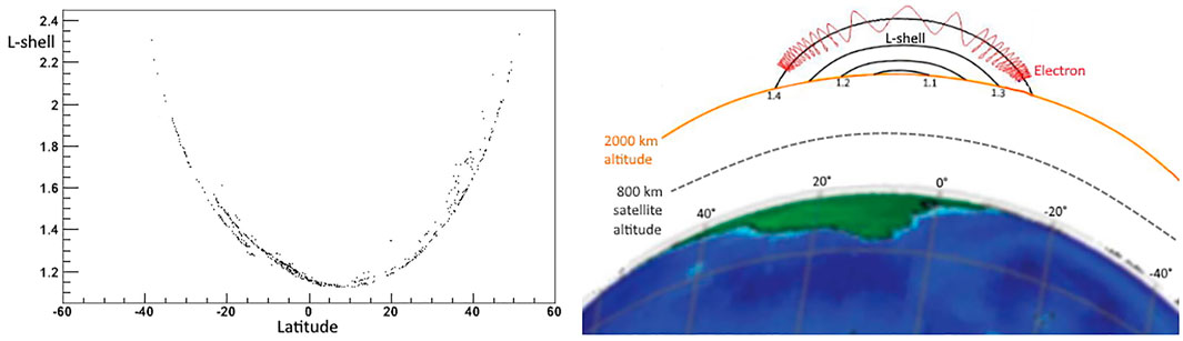
FIGURE 2. L_EB dependence by the EQ latitudes which are considered for the correlation calculus when the L_EQ at some altitude projection of the EQ epicenter is near L_EB, on the left. The parable gives a quadratic dependence. The cause of this dependence is shown on the right where the L_EB covers the expected interval, around 2,000 km of altitude above the EQ latitudes. The satellite altitude at the corresponding longitudes is well under the Van Allen Belts; the satellite altitude will approach the L_EB interval at least 60° further east.

To verify the validity of the new EB condition, a correlation was recalculated between EQs and EBs, which now includes only EB parameters, with the $L_{EB}$ being in a restricted interval. After a complete study to maximize the correlation with respect to many EQ and EB parameters, the validity of the new condition was confirmed by choosing EBs with the following: $1.21\le L_{EB}\le 1.31$, pitch angles $56°\le \alpha \le 74°$ and $108°\le \alpha \le 126°$, and positions $-35°\text{ to }15°$ in latitudes and $230°-280°$ in longitudes. For EQs, the depth must be less than 200 km, the latitude in the $-6°\text{ to }26°$ interval, and the longitude in the $90°-170°$ interval. The correlation was defined by filling the histogram ${\displaystyle {\sum }_{\left\{EQ;EB\right\}}\left(EQ\times EB\right)}$ with the differences $\Delta t=T_{EQ}-T_{EB}$ between the EQ time $T_{EQ}$ and the EB time $T_{EB}$, only for those EBs with L in the interval 1.21–1.31. The correlation was also optimized according to both the time binning and the time shift. The optimization corresponded to the $\Delta t=1.5-3.5\text{h}$ interval. Here, the time difference interval, used as the binning, was suggested as the time necessary for the EB to cover the EQ longitude interval of 80° for a 60-keV electron drifting eastward at $L=1.26$, which was found to be about 2 h. After it, the number of correlation events is increased to 44, thus improving the correlation significance. The updated correlation is shown in Figure 3 (left), and the geographical distribution of correlated EQs is shown on the right. $L_{EB}$ and the EB geographic position were found to be the critical parameters to reveal EB true alarms, and the $\Delta t=1.5-3.5\text{h}$ interval is used from here on out. It should be noted that the peaks around 48 h and around 0 h are consistent with the results of the study by Anagnostopoulos et al. (2012), even if with a low significance.

FIGURE 3

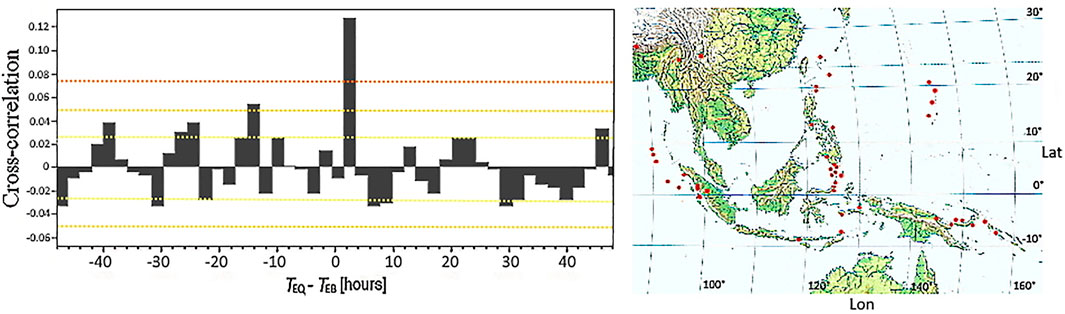
FIGURE 3. Pearson’s cross correlation between EBs and EQs recalculated using the new condition on L_EB for 16.5 years of data is shown on the left; the 1 σ, 2 σ, and 3 σ thresholds are indicated by yellow, orange, and red dotted lines, respectively. The Indonesian and the Philippine strong EQs producing the 1.5–3.5-h correlation peak are shown on the right.

Forecasting Methodologies

Following a work by Fidani (2018), the conditional probability of a strong EQ, given the EB measurement, can be calculated using the relation between the covariance and cross correlation (Billingsley, 1995). Moreover, this discussion is valid for binary events using any physical observation other than the EB, which is correlated with the EQ. If applied to the EQ and EB unitary events, the binary correlation is as follows:

$corr\left(EQ,EB\right)=\frac{\mathit{cov}\left(EQ,EB\right)}{\sqrt{P\left(EQ\right)\left[1-P\left(EQ\right)\right]P\left(EB\right)\left[1-P\left(EB\right)\right]}},(1)$

where the $\mathit{cov}\left(EQ,EB\right)=\left[P\left(EQ\cap EB\right)-P\left(EQ\right)P\left(EB\right)\right]$ can be explicated throughout the histogram of the EQ to EB coincidences ${\displaystyle {\sum }_{\left\{EQ;EB\right\}}\left(EQ\times EB\right)}$ in the following population formula:

$\mathit{cov}\left(EQ,EB\right)=\frac{N_h{\displaystyle {\sum }_{\left\{EQ;EB\right\}}\left(EQ\times EB\right)}-N_{EQ}{N}_{EB}}{N_h^2},(2)$

where $N_{EQ}$ and $N_{EB}$ are the number of EQs and EBs that participated in the correlation, respectively, while $N_h$ is the number of total hours divided by two considered for the correlation. Being so, the probabilities of single events are $P\left(EQ\right)=N_{EQ}/N_h\text{ and }P\left(EB\right)=N_{EB}/N_h$. The binary correlation histogram is then calculated as follows:

$corr\left(EQ,EB\right)=\frac{{\displaystyle {\sum }_{\{EQ;EB\}}\left(EQ\times EB\right)}/N_h-P\left(EQ\right)P\left(EB\right)}{\sqrt{P\left(EQ\right)\left[1-P\left(EQ\right)\right]P\left(EB\right)\left[1-P\left(EB\right)\right]}}.(3)$

Being the joint probability by definition of the covariance and from Eq. 1, we have the following:

$P\left(EQ\cap EB\right)=P\left(EQ\right)P\left(EB\right)+corr\left(EQ,EB\right)\sqrt{P\left(EQ\right)\left[1-P\left(EQ\right)\right]P\left(EB\right)\left[1-P\left(EB\right)\right]}.(4)$

The conditional probability $P\left(EQ|EB\right)=P\left(EQ\cap EB\right)/P\left(EB\right)$ can be rewritten as follows:

$P\left(EQ|EB\right)=P\left(EQ\right)+corr\left(EQ,EB\right)\sqrt{\frac{P\left(EQ\right)\left[1-P\left(EQ\right)\right]\left[1-P\left(EB\right)\right]}{P\left(EB\right)}}=\frac{{\displaystyle {\sum }_{\left\{EQ;EB\right\}}\left(EQ\times EB\right)}}{N_{EB}}.(5)$

which means that if a correlation exists between EQs and EBs which is ${\max }_{\Delta t}\left[{\displaystyle {\sum }_{\left\{EQ;EB\right\}}\left(EQ\times EB\right)}\right]$ and the time difference $\Delta t$ between EQ and EB is chosen to be that of correlations, the probability of an EQ with M ≥ 6 is increased by a term proportional to the correlation.

An equivalent approach to test the results obtained using NOAA particle data refers to the work by Console (2001). Here, a simple definition of an EQ forecasting hypothesis was suggested with a particular sub-volume of the total time–space volume, called the alarm volume, within which the probability of occurrence of strong EQs is higher than the average. Following the work by Console, the prediction related to the detection of a precursor consists in the occurrence of an EQ event of minimal magnitude in the alarm volume. In this framework, the performance of a specific method is carried out through the statistical parameters that can be evaluated in this example, such as the success rate $N_S/N_A$, the false alarm rate $\left(N_A-N_S\right)/N_A$, the alarm rate $N_S/N_E$, the failure rate $\left(N_E-N_S\right)/N_E$, and the probability gain (Console, 2001), as shown below:

$G=\frac{N_S}{N_A{V}_A}\frac{V_T}{N_E},(6)$

where $N_S$ is the success number, $N_A$ is the alarm number, $N_E$ is the EQ number, $V_A$ is the alarm volume, and $V_T$ is the total volume. It should be noted that this description is completely equivalent to the previous being $N_S={\max }_{\Delta t}\left[{\displaystyle {\sum }_{\left\{EQ;EB\right\}}\left(EQ\times EB\right)}\right]$, $N_A=N_{EB},N_E=N_{EQ},V_A=A·N_h$, where A is the Indonesian and Philippine areas and $V_A=2A$ is for the alarm duration of 2 h. $V_A$ based on NOAA particle data is constant for all the alarms. Thus, the success rate is exactly $P\left(EQ|EB\right)$, the false alarm rate is $1-P\left(EQ|EB\right)$, the alarm rate is ${\max }_{\Delta t}\left[{\displaystyle {\sum }_{\left\{EQ;EB\right\}}\left(EQ\times EB\right)}\right]/N_{EQ}$, the failure rate is $1-{\max }_{\Delta t}\left[{\displaystyle {\sum }_{\left\{EQ;EB\right\}}\left(EQ\times EB\right)}\right]/N_{EQ}$, and the probability gain is as follows:

$G=\frac{P_{\Delta t}\left(EQ|EB\right)}{P\left(EQ\right)}=1+cor{r}_{\Delta t}\left(EQ,EB\right)\sqrt{\left[1/P\left(EQ\right)-1\right]\left[1/P\left(EB\right)-1\right]},(7)$

where $cor{r}_{\Delta t}\left(EQ,EB\right)$ is the particular correlation and $P_{\Delta t}\left(EQ|EB\right)$ is the particular conditional probability, both corresponding to a $\Delta t$ of 1.5–3.5 h.

Evaluating Significance

A criterion for considering one model more valid than another can be made through the log-likelihood of observing that particular realization of the EQ process: under the hypothesis defining the probabilities of occurrence in P sub-volumes p_i, and c_i being the digital occurrence of at least one event in the sub-volume, the following is the case (Console, 2001):

$\log \left(L\right)={\displaystyle \sum _{i=1}^P\left\{c_i\log \left[p_i/\left(1-p_i\right)\right]-\log \left(1-p_i\right)\right\}}.(8)$

The geographical regions of Indonesia and the Philippines are considered, where strong $\left(M\ge 6\right)$ EQs occurred over 16.5 years from July 1998, which were correlated with the NOAA EBs. The space–time alarm sub-volumes are in this case disjointed and separated in time only, each completely covering both areas for 2-h time intervals from 1.5 to 3.5 h after the EB observations. If so, the complete volume covers N_h hours, of which N_EQ are those where an EQ occurred with $c_i=1$, $N_{EB}$ are those where an alarm occurred with $p_i=P\left(EQ|EB\right)$, $N_h-N_{EB}$ are those where no alarm occurred with $p_i=P\left(EQ\right)$, and ${\displaystyle {\sum }_{\left\{EQ;EB\right\}}\left(EQ\times EB\right)}$ are those where an EQ followed an alarm and where $p_i=P\left(EQ|EB\right)$. The log-likelihood histogram is as follows:

$\begin{array}{l}\log \left(L\right)=\log \left[\frac{P\left(EQ|EB\right)}{1-P\left(EQ|EB\right)}\right]{\displaystyle {\sum }_{\{EQ;EB\}}\left(EQ\times EB\right)}\\ +\left[N_{EQ}-{\displaystyle {\sum }_{\{EQ;EB\}}\left(EQ\times EB\right)}\right]\log \left[\frac{P\left(EQ\right)}{1-P\left(EQ\right)}\right]\\ +\hspace{0.17em}{N}_{EB}\log \left[1-P\left(EQ|EB\right)\right]+\left(N_h-N_{EB}\right)\log \left[1-P\left(EQ\right)\right],\end{array}(9)$

and it is possible to compare this forecasting hypothesis with a simpler model, called the null hypothesis, that is, the Poisson hypothesis. The success rate of this model is constantly $P\left(EQ\right)$ and the probability gain is always $G=1.0$, so that the log-likelihood is calculated as follows:

$\log \left(L_0\right)=N_{EQ}\log \left[P\left(EQ\right)\right]+\left(N_h-N_{EQ}\right)\log \left[1-P\left(EQ\right)\right].(10)$

The log-likelihood ratio (Martin, 1971) can now be calculated to test the near-Earth space influence hypothesis against the null hypothesis for $\Delta t$ of the maximum correlation, evaluating the following:

$\begin{array}{l}\log \left(\frac{L_{\Delta t}}{L_0}\right)={\max }_{\Delta t}\left[{\displaystyle {\sum }_{\left\{EQ;EB\right\}}\left(EQ\times EB\right)}\right]\log \left[\frac{P_{\Delta t}\left(EQ|EB\right)}{P\left(EQ\right)}\right]\\ +\left\{N_{EB}-{\max }_{\Delta t}\left[{\displaystyle {\sum }_{\left\{EQ;EB\right\}}\left(EQ\times EB\right)}\right]\right\}\times \log \left[\frac{1-P_{\Delta t}\left(EQ|EB\right)}{1-P\left(EQ\right)}\right].\end{array}(11)$

Moreover, the statistical link between EQs and EBs was tested for its significance, starting from their correlation distribution (Fidani, 2015). In the work by Fidani et al. (2010), it was reported that the EQ-to-EB correlation histogram (Eq. 3), obtained collecting ${\displaystyle {\sum }_{\left\{EQ;EB\right\}}\left(EQ\times EB\right)}$ for many time differences, can satisfy a Poissonian process when only main shock EQs and semi-orbit EBs are used. Then, indicating the average correlation histogram with Ave, the standard deviation histogram is $\sigma =\sqrt{Ave}$. Being so, the number of standard deviations $N_{\sigma }$ relative to $\Delta t$, which is shown in Figure 4 of the work by Fidani (2015) for a $\Delta t$ lasting 2–3 h with respect to altitude projections, can be evaluated by calculating $Av{e}_{\Delta t}$ and ${\sigma }_{\Delta t}$ for the same $\Delta t$ as follows:

$N_{\sigma }=\frac{{\max }_{\Delta t}\left[{\displaystyle {\sum }_{\left\{EQ;EB\right\}}\left(EQ\times EB\right)}\right]-Av{e}_{\Delta t}}{{\sigma }_{\Delta t}}.(12)$

FIGURE 4

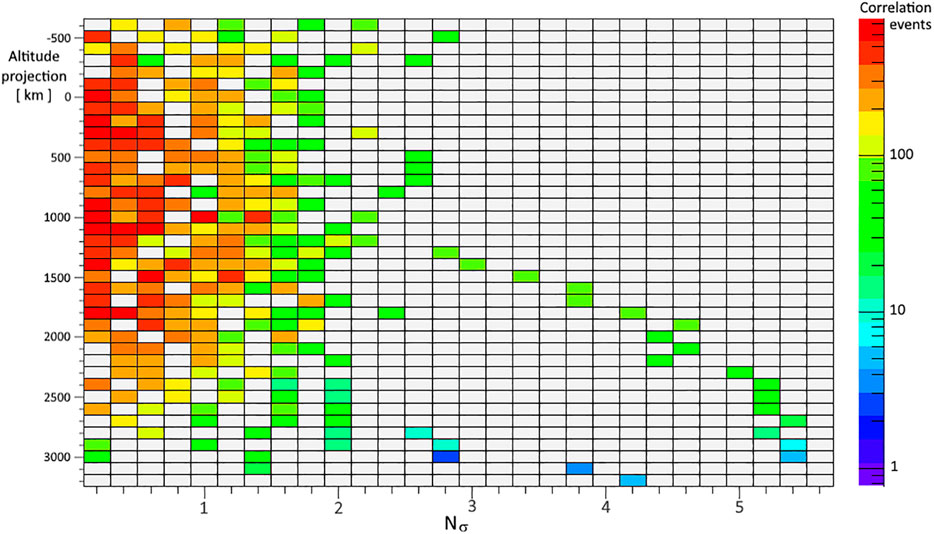
FIGURE 4. Half of the significance histogram of the correlations in Figure 1 between EBs and EQs obtained between −72 and 72 h and projecting the EQ epicenters between −600 and 3,200 km. The other half of the significance histogram concerns the negative N_σ values which have shown no anticorrelations till date. The correlation event palette on the right provides the number of EQs that contributed to that significance bin. Noteworthily, the correlation starts to be significant for altitude projections above 1,400 km, even if the maximum number of total events is reached around 1,000 km (see Figure 1).

The significance in terms of $N_{\sigma }$ is shown in Figure 4 for the entire interval of altitude projections corresponding to Figure 1. The significance ${\alpha }_{corr}$ in terms of $N_{\sigma }$ can be obtained using tables of Poisson probabilities. The significance of the new correlation was also evaluated using $N_{\sigma }$. The maximum obtained $N_{\sigma }=5.4$ corresponded to a probability $\text{< 0}\text{.}1\text{\%}$, not being a statistical fluctuation. A summary of the correlation calculated using Eq. 3, time interval $\Delta t$ and probability gains calculated using Eq. 7, and number of events and $N_{\sigma }$ calculated using Eq. 12, corresponding to the altitude projections and to the new model based on $L_{EB}$ only, are reported in columns 2, 3, 4, 5, and 6 of Table 1, respectively. The values of significance calculated using tables starting from Eq. 12 are also reported in column 7 of Table 1.

TABLE 1

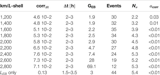
TABLE 1. Numerical values for the cross correlations corresponding to different altitudes, from 1,200 to 2,800 km, and the L_EB condition, plus their corresponding correlations, Δt, gain, number of events, and sigmas and α_corr significance.

Precursory information can be evaluated using Molchan’s error diagram (Molchan, 2003). The quantities needed to characterize the predictive properties of a strategy in an interval $\left(0,T\right)$ are the relative number of failures to predict for an EQ magnitude greater than M, as follows:

$\nu =\frac{1}{N\left(T\right)}{\displaystyle \sum _{0<t<T}\left[1-D_e\left(t\right)\right]dN\left(t\right)},(13)$

and the relative alert time is as follows:

$\tau =\frac{1}{T}{\displaystyle {\sum }_{0<t<T}{D}_e\left(t\right)t_a},(14)$

where $t_a$ is the alert time, $N\left(t\right)$ is the number of seismic events in the interval $\left(0,t\right)$, $dN\left(t\right)=N\left(t+t_a\right)-N\left(t\right)=\left\{0or1\right\}$ is the number of events in the alert time interval, and $D_e$ is a decision alert which can be $\left\{0or1\right\}$ in the interval $\left(t,t+t_a\right)$. In the NOAA electron statistical results, $t_a=2\text{h}$, $N\left(T\right)=N_{EQ}$, the relative number of failures is the failure rate in the study of Console (2001), being ${\nu }_{EB}=1-{\max }_{\Delta t}\left[{\displaystyle {\sum }_{\left\{EQ;EB\right\}}\left(EQ\times EB\right)}\right]/N_{EQ}$, and the relative alert time is ${\tau }_{EB}=P\left(EB\right)$. The statistical significance ${\alpha }_{Molch}$ of a given point $\left({\nu }_{EB},{\tau }_{EB}\right)$ on the Molchan’s error diagram can be tested using the random probability of the Poisson model, which is the diagonal of the Molchan’s diagram, and is given by the binomial distribution (Kossobokov, 2006) as follows:

$B\left[N_{EQ}\left(1-{\nu }_{EB}\right)|N_{EQ},{\tau }_{EB}\right]=C\left[N_{EQ};N_{EQ}\left(1-{\nu }_{EB}\right)\right]\times {{\tau }_{EB}}^{N_{EQ}}{\left(\frac{1}{{\tau }_{EB}}-1\right)}^{N_{EQ}{\nu }_{EB}}.(15)$

In light of this, the probability of obtaining $N_{EQ}\left(1-{\nu }_{EB}\right)$ or more hits by chance, as there have been $N_{EQ}$ observed target EQs, is described by the following:

${\alpha }_{Molch}={\displaystyle \sum _{n=m}^{N}B\left[n\mathrm{ }|N_{EQ},{\tau }_{EB}\right]},(16)$

which produces the confidence bounds and where the index $m={\max }_{\Delta t}\left[{\displaystyle {\sum }_{\left\{EQ;EB\right\}}\left(EQ\times EB\right)}\right]$. G on the Molchan’s error diagram is the slope of the line connecting $\left(\mathrm{0,1}\right)$ to $\left({\tau }_{EB},{\nu }_{EB}\right)$ (Zechar and Jordan, 2008), and it is simply calculated as $G=\left(1-{\nu }_{EB}\right)/{\tau }_{EB}$ (Molchan, 1991), which is identical to Eq. 7.

Results

The EQ prediction model analyzing the EBs detected using NOAA satellites can now be represented following the more general work by Console (2001). Thus, the recent forecasting results obtained in the work by Fidani (2020) using annual averages must be redefined, in order to fit this more general representation. Subsequently, the final assessment of the hypothesis validity should be carried out via a test on a new and independent set of observations (Console, 2001).

Prediction Model

The scenario representing the model of EQ prediction needs to define volumes where EQs occur, where the target volume V_T is 2-d space + 1-d time–space. In this volume, the points of EQ occurrence can be identified, together with alarm volumes V_A, as success (S) and failure of prediction (F) events that are EQs occurring inside or outside V_A, respectively. In this case, a precursor volume V_P containing the alarm events must be defined, which is generally different from V_T; V_P is the volume of the area where EB detection using NOAA satellites occurs, multiplied by the time of EB observations. An EB detection in V_P is an alarm event which defines V_A. With regard to the correlation mentioned above, for the Indonesian and Philippine latitudes and longitudes, V_T is obtained by multiplying this area by the time spanned by the EQ observations. In this scenario, the occurrence of an EQ event is considered only with M above a magnitude threshold $M_0$, where $M_0=6$. Unlike the models that consider EQs as precursors themselves, in this model, the EB precursor events are detected at different latitudes and longitudes, with respect to those of EQs. Correlations between EBs and EQs occurred for EB detection in the area to the west of the South Atlantic Anomaly. Thus, V_T concerns the longitude interval of 90°–170° and the latitude interval of −6°–26° multiplied by the time interval of the analysis, whereas V_P concerns the area of 230°–280° in longitude and the area of −35°–15° in latitude multiplied by the time interval of the analysis. V_A is generated by an observation of one EB in V_P. It has the same area as V_T multiplied by a duration T = 2 h, which results in the width of the correlation peak, occurring over the next 1.5–3.5 h, which is found to be the time position of the correlation peak. In this case, the alarm volume V_A is constant for all alarms. A success is added if an EQ with $M\ge 6$ occurs in the V_A. A failure is added if an EQ occurs out of the V_A, which means not included in the time intervals, and any alarm EB not followed by EQ is classified as a false alarm. The described model can be represented by the three-dimensional space of geographical coordinates and time reported in Figure 5. Performance of the NOAA EB detection is conditioned by a V_P which is not continuous. In fact, as reported above, only a low number of days are magnetically calm enough to be used for the analysis. Moreover, the NOAA satellites go into the detection area west of the South Atlantic Anomaly intermittently, thus further reducing the total time of observations.

FIGURE 5

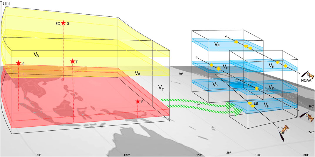
FIGURE 5. Volume representation where the forecasting model can be tested is delimited by the product among the geographical coordinates of EQs and EBs and the time of observations. V_T, V_A, and V_P are all discontinuous volumes in time as the EB analysis is suitable for EQ forecasting when the solar activity is very low. Moreover, the alarm duration is 2 h. V_T and V_A cover the entire West Pacific area, and V_P covers the different geographical areas on the western North American and South American coasts. The causal link between EQ disturbance and EB measurement events is represented by green dashed arrows. The possible precursor volume due to a hypothetical physical action on the ionosphere above the epicenters of the earthquakes is represented in red.

This is the cause of a noncontinuous V_T, where V_A appears to fill the same geographical area as V_T for a time interval of 2 h. A V_A within V_T is generated 1.5 h after an EB is observed in V_P. This is different from the model based exclusively on seismic activity, where the causal link between V_A and the precursor is near the vertical, given the seismic properties to cluster. The causal link between V_A and the EB observation event is represented near the horizontal. This causal link is the eastward electron drift, according to the electron energy, which is represented in Figure 5 by green thick arrows moving according to the longitude. The vertical distance between the starting point of arrows above the EQ epicenters and the base of V_A is the time anticipation of a possible physical interaction relating the EQ preparation volume to the ionosphere. In the analysis of 16.5 years of NOAA data, V_T concerned only the Indonesian and the Philippine areas multiplied by $N_h=\mathrm{6,953}\text{h}$. It should be noted that this value and the following are different from those reported in past publications (Fidani, 2020), as the past reports were rough estimates. In this volume, the following occurred: a total number $N_{EQ}=N_E=600$ of EQs with $M\ge 6$, a total number $N_{EB}=N_A=\mathrm{1,892}$ of alarms, and a total number $N_S=44$ of success. Being so, the success rate of this model is $N_S/N_A=0.023$, the false alarm rate is $1-\left(N_S/N_A\right)=0.977$, the alarm rate is $N_S/N_E=0.073$, the failure rate is $1-\left(N_S/N_E\right)=0.927$, and the $G=3.0$.

Here, the target volume is subdivided into nonoverlapping sub-volumes with time intervals of a day that fill V_T completely. For each day sub-volume, the probability of occurrence of at least one target event is estimated to be equal to $P\left(EQ\right)$ with no EB observed and $P\left(EQ|EB\right)$ with one EB. Analyzing the data, days with more than one burst can be found with a frequency of about 20%. These bursts can be far away in time when the time difference is more than 10,000 s (∼2.8 h) or neighbors when the time difference is 5,000–7,000 s (∼1.4–2.0 h); in the latter case, they belong to successive orbits according to NOAA POES orbit parameters. It should be remembered that all EBs in a semi-orbit were considered as only one EB to be counted for the correlation calculus (Fidani, 2015). When two bursts are far away, the time alarm of the first ends before the beginning of the second detection, so two disjoint V_A with the same increasing of the conditional probabilities occur. When detected bursts belong to successive orbits, the V_A time interval of 2 h is greater than the range of 5,000–7,000 s, and a partial overlapping between two consecutive alarms will also occur. The few cases of overlapping for NOAA alarms are not considered here and will be presented in a future publication.

Dependent Observables

Bayes’ theorem allows us to compute the probability that a hypothesis is true, provided that one knows the probable truth of all supporting arguments. It reverses the conditional probabilities and defines the probability of the hypothesis given the evidence. It shows that there is a significant probability gain in using precursors for prediction, even if a phenomenological occurrence is not the proof of a precursor. However, starting from the correlation results (Fidani, 2015), Bayes’ theorem, as shown below,

$P\left(EB|EQ\right)=\frac{P\left(EB\right)\mathrm{ }P\left(EQ|EB\right)}{P\left(EQ\right)},(17)$

can be employed using statistical bases (Eq. 5). Being so, the alarm rate can be rewritten as $P\left(EB|EQ\right)$, the failure rate as $1-P\left(EB|EQ\right)$, and the probability gain as follows:

$G_{EB}=\frac{P\left(EB|EQ\right)}{P\left(EB\right)}=G.(18)$

Bayes theorem allows us to compute the probability of an EB given the measurement of an EQ. If calculated, it appears surprisingly high, equal to 0.8 for the correlation. However, this result must not be misinterpreted. In fact, the probability gain remains the same, suggesting that the high probability of detecting an EB when an EQ is observed is due to its greater frequency of EB occurrence.

Bayes’ theorem tests hypotheses and can be updated on the basis of new information. If used under the condition of many independent precursors EB, EC, ED …, the EQ conditional probability in a small time interval of a given area after the simultaneous detection of one EB, one EC, one ED ... can be approximated by (Aki, 1981) the following:

$P\left(EQ|EB\cap EC\cap ED\cap \mathrm{...}\right)\simeq P\left(EQ\right)G_{EB}{G}_{EC}{G}_{ED}···.(19)$

It is the product among the unconditional probability and the probability gains of each precursor; those are the ratios between the conditional probability of each precursor and unconditional probability. However, the condition of independent precursors is difficult to prove, and from the studies reported in the Introduction, a set of physical links for only a part of them is suspected (see, for example, the study by Pulinets et al. (2015)). Therefore, it seems that dependent candidate precursors represent the most common occurrence. Therein, the conditional probability of an $EQ$ with a magnitude greater than $M_0$ is not increased by a product of a further probability gain of another detected precursor, if this has a certain degree of dependence on the first to be detected. Thus, the conditional probability cannot be approximated by Eq. 19; it must be recalculated. Starting with only two dependent precursors $EB$ and $EC$ that generate alarms in the same $V_T$, the conditional probability on $EQ$, given the observations of both precursors $EB$ and $EC$, can be expressed using the relations (Eq. 7) and (Eq. 1) as follows:

$G_{EB\cap EC}=1+\frac{\mathit{cov}\left(EQ,EB\cap EC\right)}{P\left(EQ\right)P\left(EB\cap EC\right)},(20)$

where the covariance can be explicated throughout the histogram of $EQ$ to $EB\cap EC$ coincidences ${\displaystyle {\sum }_{\left\{EQ;EB\cap EC\right\}}\left[EQ\times \left(EB\wedge EC\right)\right]}$, and by considering the total number $N_{EB\cap EC}$ of correlated precursor events. Finally, $P\left(EB|EC\right)$ can be calculated through the $corr\left(EB,EC\right)$ of the relation (Eq. 5), as with all the other conditional probabilities. However, a more interesting question might arise upon using two observation networks whose observables are dependent: what is the overall probability gain upon using observations without differentiating them? In this case, the warning corresponds to a detection from the set of dependent observables $EB\cup EC$, which means that the probability, as shown below,

$P\left(EQ|EB\cup EC\right)=\frac{P\left(EQ\cap \left(EB\cup EC\right)\right)}{P\left(EB\cup EC\right)},(21)$

is conditioned by the observation of an EB or an EC or of both an EB and an EC, indifferently. Then, using simple algebra with $P\left(EQ\cap \left(EB\cup EC\right)\right)=P\left(\left(EQ\cap EB\right)\right)\cup \left(EQ\cap EC\right))$, we obtain the following:

$P\left(EQ|EB\cup EC\right)=\frac{P\left(EQ\cap EB\right)+P\left(EQ\cap EC\right)-P\left(EQ\cap EB\cap EC\right)}{P\left(EB\right)+P\left(EC\right)-P\left(EB\cap EC\right)},(22)$

where $P\left(EQ\cap EB\right)=P\left(EQ|EB\right)P\left(EB\right)$, $P\left(EQ\cap EC\right)=P\left(EQ|EC\right)P\left(EC\right)$, $P\left(EB\cap EC\right)=P\left(EB|EC\right)P\left(EC\right)$, $P\left(EQ\cap EB\cap EC\right)=P\left(EQ|EB\cap EC\right)P\left(EB\cap EC\right)$. Considering the relation (Eq. 7), the probability gain due to the observation of an event in $EB\cup EC$ is as follows:

$G_{EB\cup EC}=\frac{G_{EB}P\left(EB\right)+[G_{EC}-G_{EB\cap EC}P\left(EB|EC\right)]P\left(EC\right)}{P\left(EB\right)+[1-P\left(EB|EC\right)]P\left(EC\right)},(23)$

where $G_{EB}$ and $G_{EC}$ are the probability gains of the single precursor $EB$ and the single precursor $EC$, respectively. $G_{EB\cap EC}$ is the probability gain (Eq. 20) due to the observation of both $EB$ and $EC$ events that are correlated between them. Alternatively, using the relations (Eq. 7) and (Eq. 1), we obtain the following:

$G_{EB\cup EC}=1+\frac{\mathit{cov}\left(EQ,EB\cup EC\right)}{P\left(EQ\right)P\left(EB\cup EC\right)},(24)$

where the covariance can be explicated throughout the histogram of $EQ$ to $EB\cup EC$ coincidences ${\displaystyle {\sum }_{\left\{EQ;EB\cup EC\right\}}\left[EQ\times \left(EB\vee EC\right)\right]}$, and by considering the total number $N_{EB\cup EC}=N_{EB}+N_{EC}-N_{EB\cap EC}$.

Different Precursors Combined

It needs to be highlighted that a statistical correlation between the two time series does not generally mean that they are physically related (Aldrich, 1995). A causal link has been hypothesized between EB measurements and EQ occurrence (Fidani, 2018; 2020), which supports the validity of the hypothesis. Although the $\Delta t=T_{EQ}-T_{EB}$ time difference of the correlation is in agreement with the physical migration of electrons eastward, this migration has not yet been observed for EBs correlated with EQs. Furthermore, a physical link between the EQ preparation zone and the ionosphere above the future epicenter, separated by about 2,000 km, has not been demonstrated. Finally, the existence of some physical phenomena occurring at the future EQ epicenter, which is enough to influence the ionosphere, remains only a hypothesis until all of these passages have been fully demonstrated. To discover EBs with the correct times at different longitudes, which would satisfy their physical migration in the ionosphere, more satellites are needed. This verification is currently possible for EBs, as different NOAA satellites fly together, even though cases having suitable satellite positions must be found. Till date, this has not been calculated, as no correlations have been found with EBs selected using other satellite databases during the same periods.

Regarding a physical link, able to cover more than 2,000 km between the Earth’s crust and the ionosphere throughout the atmosphere, magnetic pulses have been hypothesized to influence the high-energy charged particles’ motion by pitch angle diffusion (Galper et al., 1995). Even if other processes have been proposed more recently, such as the injection of radioactive substances and charged aerosols into the atmosphere, leading to a change in the vertical electric current in the atmosphere and to a modification of the electrical field in the ionosphere (Sorokin et al., 2001), from a solid-state physics perspective (Freund, 2011), and radioactive ionization to model the lithosphere–atmosphere–ionosphere–magnetosphere coupling by the latent heat flux (Pulinets et al., 2015), by AGW (Yang et al., 2019; Piersanti et al., 2020). Recent measurements of magnetic pulses on the occasions of strong EQs (Bleier et al., 2009; Orsini, 2011; Nenovski, 2015) have suggested an efficient process which may influence the ionosphere (Fidani et al., 2020). In this latter work, the magnetic data analysis at the Chieti Station of the Central Italy Electromagnetic Network, performed using two independent sample systems of the same signal, showed that a large number of pulses were recorded in the ELF band below 10 Hz with amplitudes mostly in the range of 2.5–80 nT. Specifically, the model proposed for analyzing magnetic pulses consisted of diffused underground electrical currents throughout a conductive strip between the Apennines and the Adriatic Sea. The current required to induce detected pulses is greater than i = 40 kA for the strongest pulses. Unipolar magnetic pulses can be, for example, generated deep in the rock column by peroxy defects when rocks are subjected to increasing deviatoric stresses (Freund et al., 2021). The proposed strip of diffuse current constitutes the electromagnetic source of ULF waves, which is able to produce low intensities of magnetic inductions on the Earth’s surface, even if it is measurable both near and far from the EQ epicenter. The strip of diffuse current is able to produce significant fields, also far from the ground by integration. To demonstrate this and calculate magnetic induction in the ionosphere, two simple models can be considered. An infinitely long strip of about 6-km-thick and 150-km-large conductive soil has been considered to calculate the magnetic induction very close to the larger strip surface. In a real case, a finite-length strip should be utilized, which gives a correct result even for a coil magnetometer very close to the strip. Referring to Figure 6, on the left side, where the lines of induction are generated by a not-finite strip and wire lengths are compared, it is possible to see that the B intensities near the strip are lower than those near the wire. This is due to the current density differences flowing near the observational point. Relations (Eq. 2) and (C4) of the study by Fidani et al. (2020) were used for the wire and the strip, respectively. Moving away from the current density, magnetic inductions generated by the wire and the strip become equal, when the distance overcomes the strip width. However, currents which are not of finite length deviate too much from the real case at large distances. So, a finite length l of the wire is considered and the magnetic induction is simply calculated as follows:

$B=\frac{{\mu }_{o}il}{4\pi d\sqrt{\left(d^2+l^2\right)}},(25)$

where d is the distance. Figure 6, on the right side, depicts a comparison of B intensities of the two models with the distance. The B intensity results are limited to 0.2 nT at distances of 1,000 km with a total current of 40 kA. This is in agreement with the intensities obtained from the theoretical calculations, which have shown that only a magnetic type source with frequency < 10–20 Hz can be effective for the penetration of fields into the upper ionosphere and magnetosphere (Molchanov et al., 1995). Moreover, magnetic disturbances were observed above moderate EQ epicenters for the frequency band of 0.1–10 Hz (Strakhov et al., 1994). From the upper ionosphere, these waves travel as Alfven waves further along the geomagnetic field line and reach the inner boundary of the inner Van Allen Belt. Alfven waves are thought to resonantly interact with trapped charged particles; this process is most intensive in the equatorial part of the magnetosphere, for L-shell values equal to or less than 2 (Molchanov and Mazhaeva, 1993). In fact, the measured pulse frequency under 10 Hz is around the bouncing resonance of electrons with energies between 30 and 100 keV (Walt, 1994); it is exactly as measured on board NOAA satellites. This means that energy can be efficiently transferred from magnetic pulses producing electron pitch angle disturbances (Galper et al., 1995). Furthermore, the B intensity due to an Earth surface strip of current is a very low value, compared to an example of geomagnetic activity. However, the frequency range of geomagnetic activity is about 0.0001–0.01 Hz (Francia and Villante, 1997), so that the B rate is out of resonance. Finally, currents produced by lightning are generally lower in intensity, around i = 10 kA, with frequency emissions in the upper part of the ELF band and the VLF band still out of bouncing resonance (Inan et al., 2010).

FIGURE 6

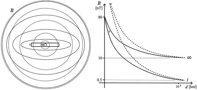
FIGURE 6. Comparison of magnetic induction lines produced by the rectangular and circular sections in the center on the left; continuous lines are generated by the rectangular strip (s), whereas the dotted lines are generated by the wire (w). B dependence, from the distance at half of the strip width of the currents, is shown on the right for both conductors that are infinitely long or of length l using the relation (Eq. 25) and the relation (Eq. 2) of the study by Fidani et al. (2020).

Indeed, magnetic signals have been correlated with strong EQs in different regions of the world such as Japan (Ohta et al., 2013), Kamchactka (Schekotov et al., 2019), and California (Kappler et al., 2019). The Japanese and Kamchactka studies obtained correlations with time differences of 2–5 days before seismic events, and probability gains of about 1.6 (Han et al., 2014) to 2.6 (Hayakawa et al., 2019) were reported. Magnetic pulses, from here on identified with ECs, have been hypothesized to induce EBs, and therefore, they may be considered dependent events for hypothesis. The relation (Eq. 23) can be used to calculate the probability gain of EQ probability due to possible observations of both EBs and ECs. This possibility can be useful as the observation of ECs on the Earth’s surface can occur when a NOAA satellite is not in a suitable position to reveal the possibly induced EBs. Moreover, magnetic detectors cannot be installed at some positions offshore or are not able to detect ECs where there are EQs. In other words, EBs and ECs can compensate for the gaps on each other in a forecasting experiment, where V_T is very large, as for the West Pacific. The magnetic pulse precursor can be represented by the red volume of Figure 5. Being so, the mutual interrelation of the sets of EBs, ECs, and EQs is a completely real case, which can be studied for a total probability gain with the expression (Eq. 23). To show the advantage in using two dependent observables, a forecasting experiment can be imagined where both EB and EC data are available. Here, one can imagine the presence of a magnetometer network distributed on several islands of the West Pacific. Although not still existent, this network is currently achievable. We suppose that it exists and is able to obtain a $G_{EC}=1.6$ for EQs within a certain distance around the stations, with a time advance of ECs of 4–6 h with respect to EQs. $P\left(EC\right)$ is necessary for Eq. 23 and is supposed to be 0.05, which means $N_{EC}=324$ magnetic pulses, or sets of magnetic pulses, considered as magnetic alarms on the same time interval as for EBs. For what concerns the NOAA observable, a $G_{EB}=3$ was found from the correlation analysis. However, even if ECs from days with the Ap index above the previously defined threshold were excluded as for EBs, the daily NOAA observation time was always half a day (Fidani, 2020) due to the satellite’s orbit crossing the EB detection region. Being so, the probability gain should be evaluated on a double time interval and being able to detect the same number of EBs. The probability gain is thus approximately $G_{EB}=1.5$. With regard to $P\left(EB|EC\right)$, the correlation between EBs and ECs would need to be calculated using observational data. $P\left(EB|EC\right)$ depends on the histogram maximum ${\max }_{\Delta t\ast }\left[{\displaystyle {\sum }_{\left\{EB;EC\right\}}\left(EB\times EC\right)}\right]$, where $\Delta t\ast =4\left(6\right)-\Delta t$ is such that the total time in advance of ECs with respect to EQs is 4–6 h. This could be chosen in the range from 0, no correlation, to 324, complete correlation, the $N_{EB}$ being a much higher number, in order to consider a range of possibilities. Concerning $G_{EB\cap EC}$, the correlation between $EQ$ and $EB\cap EC$ would need to be calculated utilizing observational data for ${\max }_{\Delta t}\left[{\displaystyle {\sum }_{\left\{Eq;EB\cap EC\right\}}\left(EQ\times \left(EB\wedge EC\right)\right)}\right]$. If $EB\cap EC$ at $\Delta t$ are the set of events EB and EC related by chance, ${\displaystyle {\sum }_{\left\{EB;EC\right\}}\left(EB\times EC\right)}$ should be a low value with $G_{EB\cup EC}\simeq \left[G_{EB}P\left(EB\right)+G_{EC}P\left(EC\right)\right]/\left[P\left(EB\right)+P\left(EC\right)\right]$. The dependence between EBs and ECs can be introduced in Eq. 23 by fixing a time shift in ECs of $\Delta t\ast$ so that the number of correlation events is $\max \left[{\displaystyle {\sum }_{\left\{EB;EC\right\}}\left(EB\times EC\right)}\right]={\max }_{\Delta t\ast }\left[{\displaystyle {\sum }_{\left\{EB;EC\right\}}\left(EB\times EC\right)}\right]$. It would also be necessary in this case to consider a range of possibilities from 0, no correlation between $EQ$ and $EB\cap EC$, to 10 common events. The probability gain improvements that are obtainable thanks to a network of EC measurements added to the NOAA satellite EB detection are reported in the contour plot of Figure 7.

FIGURE 7

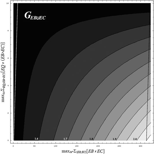
FIGURE 7. Probability gain (Eq. 23) due to the contribution of EB and EC detection, where in this case ECs are ULF magnetic pulses. This gain is calculated with respect to the maximum event correlation between EBs and ECs on the abscissa, which comes from $P\left(EB|EC\right)$, and to the maximum event correlation between $EQ$ and $EB\cap EC$ on the ordinate, which is derived from $P\left(EQ|EB\cap EC\right)$. $\Delta t\ast =T_{EB}-T_{EC}$ is thought to be the drifting time of electrons from the ionosphere above the epicenter to the cross with the NOAA satellite. Therefore, $G_{EB\cup EC}$ is described by the contours if $\Delta t$ of EB-to-EC correlation is shifted by $\Delta t\ast$, that is, the dependence between EBs and ECs. The white dotted line on the left and the black one on the right represent $G_{EB\cup EC}$ limits of validity.

The maximum value of $G_{EB\cup EC}=2.05$ is obtained for 314 ECs which are correlated with EBs, but none of these EBs are correlated with EQs, shown by point (314, 0) of Figure 7, which means that 10 ECs are correlated with EQs and another part of EBs not correlated with ECs is correlated with EQs; thus, the total number of different observations correlated with EQs is increased by 10. $G_{EB\cup EC}$ is a minimum when the correlation events between EBs and ECs are ${\max }_{\Delta t\ast }\left[{\displaystyle {\sum }_{\left\{EB;EC\right\}}\left(EB\times EC\right)}\right]=0$, shown by the point (0, 0) of Figure 7. That is, when there are no ECs correlated with EQs nor with EBs, and $G_{EB\cup EC}$ is slightly less than 1.6 because it is a weighted average between G_EB and G_EC. When the EB-to-EC correlation increases to 10 events, a maximum of 10 correlations with EQs can happen, as shown by point (10, 10) of Figure 7, where $G_{EB\cup EC}$ is still lower due to redundancy. $G_{EB\cup EC}$ does not exist to the left of the white dotted line and on the right of the black dotted line. When the EB-to-EC correlation is at the maximum and the correlation of such ECs with EQs reaches 10 events, as shown by point (324, 10) of Figure 7, $G_{EB\cup EC}$ returns as near 1.5 due to the low number of correlated EQ events.

Conclusion

A complete EQ forecasting methodology has been considered in this study based on NOAA satellite high-energy electron detection. It utilizes recently discovered correlations existing between EBs selected from the NOAA database and strong EQs collected at the USGS (Fidani, 2015), which can be classified as an electromagnetic phenomenon and a near-seismic precursor. This correlation, concerning EBs anticipating main shocks, has been obtained also thanks to the geomagnetic disturbance database of the Ap and Dst indexes, as well as the IGRF model. The methodology has been represented by the volumes of target, alarm, and precursor, for testing EQ forecast hypotheses (Console, 2001).

To systematically test this methodology, a quantitative and rigorous definition of the anomaly is given according to a statistical criterion with respect to the Poisson distribution of electron CRs. Here, electrons must be escaping the trapping conditions, that is, precipitating, probably due to a disturbance. Finally, novel in relation to previous publications (Fidani, 2015; Fidani, 2018; Fidani, 2020), the parameter L-shell of the electrons has been disentangled from apparent L-shells associated to EQs. In fact, the condition of the difference $\left|L_{EB}-L_{EQ}\right|\le 0.1$ in previous publications was substituted with the $1.21\le L_{EB}\le 1.31$, which was deduced from the correspondence between electron L-shells at around 2,000 km and EQ latitudes. This disentangling between anomalies and EQs is essential to provide a precise definition of the observed phenomenon (Wyss, 1997) in order to carry out a forecast.

The statistical correlation between EBs and EQs has been extended to a time difference of 1.5–3.5 h, thanks to the hypothesized causal connection of drifting electrons. Maximizing the significance of this correlation indicated that EQs still belong to the Indonesian and the Philippine areas, collecting more seismic events from the West Pacific. These EQs occurred as in the previous analysis, mainly in the sea, with a depth up to 200 km to correlate with EBs. Regarding EBs, the pitch angle intervals were restricted, even if the number of EBs increased. To demonstrate that the correlation calculus is completely equivalent to the frequency approach of Console (2001), the probability gain was recalculated in terms of conditional probability and correlation for digital events.

After having stressed that a statistical correlation between two time series does not generally mean that they are physically related (Aldrich, 1995), the hypothesis concerning a physical link between EBs and EQs was studied. A recent observation of magnetic pulses recorded before strong EQs in Central Italy provided recorded magnetic intensities with a diffuse current model (Fidani et al., 2020). This model can push back to the hypocenter region the causal connection of physical events, even if the deduced magnetic inductions in the ionosphere must be demonstrated to be able to modify the electron pitch angles. Being magnetic pulses measurable on the Earth’s surface, they might be precursors, and indeed, statistical correlation of magnetic pulses was found (Han et al., 2014; Hayakawa et al., 2019). However, given their possible causal link with EBs, magnetic pulses and EBs could not be independent precursors. Thus, starting from Bayes’ theorem, a more general relationship of the probability gain due to the combination of two precursors is expressed in terms of single probability gains of each precursor and the correlation between the precursors. An example of improvement in the probability gain due to a couple of digital dependent precursors is tentatively calculated for the first time. A dependence between the precursors is introduced in the probability gain (Eq. 23) by a time shift which correlates the precursors. The best probability gain is obtained for the maximum correlation between precursors not correlated with EQs.

Finally, this methodology is general enough that it could be adapted to the combinations of observations from both the Earth’s surface and space, such as electromagnetic, seismic, or other physical observables. To do this, a series of steps must be performed: 1) collect data from the same instrument(s) with the same environmental conditions for many years, 2) search for anomalies of a physical observable with a statistical rigor, following a physical idea of possible equilibrium disturbances, 3) calculate a statistical correlation between EQs and anomalies by selecting physical parameters disentangled from EQ parameters, following a physical idea of possible interaction, 4) calculate the correlation significance, or the likelihood, or the Molchan’s error diagram and optimize it with respect to the physical parameters, 5) use the more relevant parameters to determine the correlation significance, or the likelihood, or the Molchan’s error diagram for a physical model refinement, 6) demonstrate the $\Delta t$ and $\Delta t\ast$ agreement of the two observables using a unified physical model, and 7) calculate the probability gain to one or more precursors and to their combinations, and verify the results in a target volume of future times or different databases. If step 6 is not obtained, the probability gain (Eq. 23) can be maximized with respect to $\Delta t$ and $\Delta t\ast$ to suggest a probable unified physical model. Moreover, an experiment for the EQ forecasting test in Indonesia and the Philippines is currently feasible using the NOAA-15 satellite, given the presence of the United States West Coast antennas (Fidani, 2020). This could be concluded over a few years with a reasonable response, due to the high frequency of strong seismicity in Indonesia and the Philippines.

Data Availability Statement

Publicly available datasets were analyzed in this study. This data can be found here: http://www.ngdc.noaa.gov/stp/satellite/poes/dataaccess.html; http://wdc.kugi.kyoto-u.ac.jp/dst_final/index.html; https://www.ngdc.noaa.gov/geomag/data.shtml; https://earthquake.usgs.gov/earthquakes/search/.

Author Contributions

CF: scientific analysis and manuscript writing.

Conflict of Interest

The author declares that the research was conducted in the absence of any commercial or financial relationships that could be construed as a potential conflict of interest.

Publisher’s Note

All claims expressed in this article are solely those of the authors and do not necessarily represent those of their affiliated organizations, or those of the publisher, the editors and the reviewers. Any product that may be evaluated in this article, or claim that may be made by its manufacturer, is not guaranteed or endorsed by the publisher.

References

Aki, K. (1981). “A Probabilistic Synthesis of Precursory Phenomena,” in Earthquake Prediction, an International Review, Maurice Ewing Vol. 4. Editors D.W. Simpson, and P. G. Richards (Washington, DC: AGU), 566–574.

Google Scholar

Aldrich, J. (1995). Correlations Genuine and Spurius in Pearson and Yule. Stat. Sci. 10 (4), 364–376. doi:10.1214/ss/1177009870

CrossRef Full Text | Google Scholar

Aleksandrin, S. Y., Galper, A. M., Grishantzeva, L. A., Koldashov, S. V., Maslennikov, L. V., Murashov, A. M., et al. (2003). High-energy Charged Particle Bursts in the Near-Earth Space as Earthquake Precursors. Ann. Geophys. 21, 597–602. doi:10.5194/angeo-21-597-2003

CrossRef Full Text | Google Scholar

An, Z., Zhan, Y., Fan, Y., Chen, Q., Chen, Q., and Liu, J. (2019). Investigation of the Characteristics of Geoelectric Filed Earthquake Precursors: a Case Study of the Pingliang Observation Station, China. Ann. Geophys. 62 (5), 545. doi:10.4401/ag-7982

CrossRef Full Text | Google Scholar

Anagnostopoulos, G. C., Vassiliadis, E., and Pulinets, S. (2012). Characteristics of Flux-Time Profiles, 20 Temporal Evolution, and Spatial Distribution of Radiation-belt Electron Precipitation Bursts in the Upper Ionosphere before Great and Giant Earthquakes. Ann. Geophys. 55, 21–36. doi:10.4401/ag-5365

Google Scholar

Asikainen, T., and Mursula, K. (2008). Energetic Electron Flux Behavior at Low L-Shells and its Relation to the South Atlantic Anomaly. J. Atmos. Solar-Terrestrial Phys. 70, 532–538. doi:10.1016/j.jastp.2007.08.061

CrossRef Full Text | Google Scholar

Barnhart, W. D., Hayes, G. P., and Wald, D. J. (2019). Global Earthquake Response with Imaging Geodesy: Recent Examples from the USGS NEIC. Remote Sensing 11, 1357. doi:10.3390/rs11111357

CrossRef Full Text | Google Scholar

Biagi, P. F., Ermini, A., and Kingsley, S. P. (2001). Disturbances in LF Radio Signals and the Umbria-Marche Seismic Sequence in 1997-1998. Phys. Chem. Earth (C) 26 (10-12), 755. doi:10.1016/s1464-1917(01)95021-4

CrossRef Full Text | Google Scholar

Billingsley, P. (1995). Probability and Measure. 3rd ed. New York: John Wiley & Sons.

Bleier, T., Dunson, C., Maniscalco, M., Bryant, N., Bambery, R., and Freund, F. (2009). Investigation of ULF Magnetic Pulsations, Air Conductivity Changes, and Infra Red Signatures Associated with the 30 October Alum Rock M5.4 Earthquake. Nat. Hazards Earth Syst. Sci. 9, 585–603. doi:10.5194/nhess-9-585-2009

CrossRef Full Text | Google Scholar

Bortnik, J., Cutler, J. W., Dunson, C., and Bleier, T. E. (2008). The Possible Statistical Relation of Pc1 Pulsations to Earthquake Occurrence at Low Latitudes. Ann. Geophys. 26, 2825–2836. doi:10.5194/angeo-26-2825-2008

CrossRef Full Text | Google Scholar

Bošková, J., Šmilauer, J., Tříska, P., and Kudela, K. (1994). Anomalous Behaviour of Plasma Parameters as Observed by the Intercosmos 24 Satellite Prior to the Iranian Earthquake of 20 June 1990. Stud. Geophys. Geod. 38, 213–220. doi:10.1007/bf02295915

CrossRef Full Text | Google Scholar

Clilverd, M. A., Rodger, C. J., and Thomson, N. R. (1999). Investigating Seismo-Ionospheric Effects on a Long Sub-ionospheric Path. J. Geophys. Res. 104 (A12), 171–179. doi:10.1029/1999ja900285

CrossRef Full Text | Google Scholar

Console, R. (2001). Testing Earthquake Forecast Hypotheses. Tectonophysics 338, 261–268. doi:10.1016/s0040-1951(01)00081-6

CrossRef Full Text | Google Scholar

Dautermann, T., Calais, E., Haase, J., and Garrison, J. (2007). Investigation of Ionospheric Electron Content Variations before Earthquakes in Southern California, 2003-2004. J. Geophys. Res. 112, B02106. doi:10.1029/2006JB004447

CrossRef Full Text | Google Scholar

Davis, G. (2007). History of the NOAA Satellite Program. J. Appl. Remote Sens 1, 012504. doi:10.1117/1.2642347

CrossRef Full Text | Google Scholar

De Santis, A., Marchetti, D., Pavón-Carrasco, F. J., Cianchini, G., Perrone, L., Abbattista, C., et al. (2019). Precursory Worldwide Signatures of Earthquake Occurrences on Swarm Satellite Data. Sci. Rep. 9, 20287. doi:10.1038/s41598-019-56599-1

PubMed Abstract | CrossRef Full Text | Google Scholar

Eleftheriou, A., Filizzola, C., Genzano, N., Lacava, T., Lisi, M., Paciello, R., et al. (2016). Long-Term RST Analysis of Anomalous TIR Sequences in Relation with Earthquakes Occurred in Greece in the Period 2004-2013. Pure Appl. Geophys. 173, 285–303. doi:10.1007/s00024-015-1116-8

CrossRef Full Text | Google Scholar

Evans, D. S., and Greer, M. S. (2004). Polar Orbiting Environmental Satellite Space Environment Monitor – 2: Instrument Descriptions and Archive Data Documentation, NOAA Technical Memorandum January, Version 1.4, 155.

Fidani, C., and Battiston, R. (2008). Analysis of NOAA Particle Data and Correlations to Seismic Activity. Nat. Hazards Earth Syst. Sci. 8, 1277–1291. doi:10.5194/nhess-8-1277-2008

CrossRef Full Text | Google Scholar

Fidani, C., Battiston, R., and Burger, W. J. (2010). A Study of the Correlation between Earthquakes and NOAA Satellite Energetic Particle Bursts. Remote Sensing 2, 2170–2184. doi:10.3390/rs2092170

CrossRef Full Text | Google Scholar

Fidani, C. (2015). Particle Precipitation Prior to Large Earthquakes of Both the Sumatra and Philippine Regions: A Statistical Analysis. J. Asian Earth Sci. 114, 384–392. doi:10.1016/j.jseaes.2015.06.010

CrossRef Full Text | Google Scholar

Fidani, C. (2018). Improving Earthquake Forecasting by Correlations between Strong Earthquakes and NOAA Electron Bursts. Terr. Atmos. Ocean. Sci. 29 (2), 117–130. doi:10.3319/tao.2017.10.06.01

CrossRef Full Text | Google Scholar

Fidani, C. (2019). From the Bayes Theorem to a Model of the Geomagnetic Interaction between strong Earthquakes in the Indonesian Archipelagos and Particle Data Detected by NOAA Satellites. Bologna: SIF2019, L'Aquila, atticon11779 IV-C-9.

Fidani, C. (2020). Probability, Causality and False Alarms Using Correlations between Strong Earthquakes and NOAA High Energy Electron Bursts. Ann. Geophys. 63 (5), 543. doi:10.44101/ag-7957

CrossRef Full Text | Google Scholar

Fidani, C., Orsini, M., Iezzi, G., Vicentini, N., and Stoppa, F. (2020). Electric and Magnetic Recordings by Chieti CIEN Station during the Intense 2016-2017 Seismic Swarms in Central Italy. Front. Earth Sci. 8, 536332. doi:10.3389/feart.2020.536332

CrossRef Full Text | Google Scholar

Finlay, C. C., Olsen, N., and Tøffner-Clausen, L. (2015). DTU Candidate Field Models for IGRF-12 and the CHAOS-5 Geomagnetic Field Model. Earth Planet. Sp 67. doi:10.1186/s40623-015-0274-3

CrossRef Full Text | Google Scholar

Francia, P., and Villante, U. (1997). Some Evidence of Ground Power Enhancements at Frequencies of Global Magnetospheric Modes at Low Latitude. Ann. Geophys. 15, 17–23. doi:10.1007/s00585-997-0017-2

CrossRef Full Text | Google Scholar

Freund, F. (2011). Pre-earthquake Signals: Underlying Physical Processes. J. Asian Earth Sci. 41, 383–400. doi:10.1016/j.jseaes.2010.03.009

CrossRef Full Text | Google Scholar

Freund, T. F., Heraud, J. A., Centa, V. A., and Scoville, J. (2021). Mechanism of Unipolar Electromagnetic Pulses Emitted from the Hypocenters of Impending Earthquakes. Eur. Phys. J. 230, 47–65. doi:10.1140/epjst/e2020-000244-4

Google Scholar

Galper, A. M., Koldashov, S. V., and Voronov, S. A. (1995). High Energy Particle Flux Variations as Earthquake Predictors. Adv. Space Res. 15 (11), 131–134. doi:10.1016/0273-1177(95)00085-s

PubMed Abstract | CrossRef Full Text | Google Scholar

Galperin, Y. I., Gladyshev, V. A., Jorjio, N. V., Larkina, V. I., and Mogilevsky, M. M. (1992). Energetic Particles Precipitation from the Magnetosphere above the Epicentre of Approaching Earthquake. Cosmic Res. 30, 89–106.

Google Scholar

Han, P., Hattori, K., Hirokawa, M., Zhuang, J., Chen, C.-H., Febriani, F., et al. (2014). Statistical Analysis of ULF Seismomagnetic Phenomena at Kakioka, Japan, during 2001-2010. J. Geophys. Res. Space Phys. 119 (6), 4998–5011. doi:10.1002/2014ja019789

CrossRef Full Text | Google Scholar

Han, P., Hattori, K., Zhuang, J., Chen, C.-H., Liu, J.-Y., and Yoshida, S. (2017). Evaluation of ULF Seismo-Magnetic Phenomena in Kakioka, Japan by Using Molchan's Error Diagram. Geophys. J. Int. 208, 482–490. doi:10.1093/gji/ggw404

CrossRef Full Text | Google Scholar

Hattori, K., Han, P., Yoshino, C., Febriani, F., Yamaguchi, H., Chen, C.-H., et al. (2013). Investigation of ULF Seismo-Magnetic Phenomena in Kanto, Japan during 2000-2010: Case Studies and Statistical Studies. Surv. Geophys. 34, 293–316. doi:10.1007/s10712-012-9215-x

CrossRef Full Text | Google Scholar

Hayakawa, M., Kasahara, Y., Nakamura, T., Muto, F., Horie, T., Maekawa, S., et al. (2010). A Statistical Study on the Correlation between Lower Ionospheric Perturbations as Seen by Subionospheric VLF/LF Propagation and Earthquakes. J. Geophys. Res. 115, A09305. doi:10.1029/2009ja015143

CrossRef Full Text | Google Scholar

Hayakawa, M., Schekotov, A., Izutsu, J., and Nickolaenko, A. P. (2019). Seismogenic Effects in ULF/ELF/VLF Electromagnetic Waves. Int. J. Elect. Appl. Res. 6 (2), 1–86. doi:10.33665/ijear.2019.v06i02.001

CrossRef Full Text | Google Scholar

He, L., and Heki, K. (2016). Three-dimensional Distribution of Ionospheric Anomalies Prior to Three Large Earthquakes in Chile. Geophys. Res. Lett. 43, 7287–7293. doi:10.1002/2016gl069863

CrossRef Full Text | Google Scholar

Henderson, T. R., Sonwalkar, V. S., Helliwell, R. A., Inan, U. S., and Fraser-Smith, A. C. (1993). A Search for ELF/VLF Emissions Induced by Earthquakes as Observed in the Ionosphere by the DE 2 Satellite. J. Geophys. Res. 98, 9503. doi:10.1029/92ja01533

CrossRef Full Text | Google Scholar

Inan, U. S., Cummer, S. A., and Marshall, R. A. (2010). A Survey of ELF and VLF Research on Lightning-Ionosphere Interactions and Causative Discharges. J. Geophys. Res. 115, A00E36. doi:10.1029/2009ja014775

CrossRef Full Text | Google Scholar

Kappler, K. N., Schneider, D. D., MacLean, L. S., Bleier, T. E., and Lemon, J. J. (2019). An Algorithmic Framework for Investigating the Temporal Relationship of Magnetic Field Pulses and Earthquakes Applied to California. Comput. Geosciences 133, 104317. doi:10.1016/j.cageo.2019.104317

CrossRef Full Text | Google Scholar

Ke, F., Wang, Y., Wang, X., Qian, H., and Shi, C. (2016). Statistical Analysis of Seismo-Ionospheric Anomalies Related to Ms > 5.0 Earthquakes in China by GPS TEC. J. Seismol 20, 137–149. doi:10.1007/s10950-015-9516-x

CrossRef Full Text | Google Scholar

Kon, S., Nishihashi, M., and Hattori, K. (2011). Ionospheric Anomalies Possibly Associated with M⩾6.0 Earthquakes in the Japan Area during 1998-2010: Case Studies and Statistical Study. J. Asian Earth Sci. 41, 410–420. doi:10.1016/j.jseaes.2010.10.005

CrossRef Full Text | Google Scholar

Kossobokov, V. G. (2006). Testing Earthquake Prediction Methods: “The West Pacific Short-Term Forecast of Earthquakes with Magnitude MwHRV≥5.8”. Tectonophysics 413, 25–31. doi:10.1016/j.tecto.2005.10.006

CrossRef Full Text | Google Scholar

Krunglanski, M. (2003). UNILIB Reference Manual, Belgisch Instituut Voor Ruimte –Aeronomie, Which Can Be Downloaded Together to the Library from. Available at: http://www.oma.be/NEEDLE/unilib.php/.

Google Scholar

Lam, M. M., Horne, R. B., Meredith, N. P., Glauert, S. A., Moffat-Griffin, T., and Green, J. C. (2010). Origin of Energetic Electron Precipitation >30 keV into the Atmosphere. J. Geophys. Res. 115, A4. doi:10.1029/2009JA014619

CrossRef Full Text | Google Scholar

Larkina, V. I., Migulin, V. V., Molchanov, O. A., Kharkov, I. P., Inchin, A. S., and Schvetcova, V. B. (1989). Some Statistical Results on Very Low Frequency Radiowave Emissions in the Upper Ionosphere over Earthquake Zones. Phys. Earth Planet. Interiors 57, 100–109. doi:10.1016/0031-9201(89)90219-7

CrossRef Full Text | Google Scholar

Larkina, V. I., Nalivayko, A. V., Gershenzon, N. I., Gokhberb, M. B., Liperovsky, V. A., and Shamilov, S. (1983). Observations of VLF Emission, Related with Seismic Activity on the Interkosmos-19 Satellite. Geomagn. Aeronomy 23, 684–687.

Google Scholar

Li, M., and Parrot, M. (2013). Statistical Analysis of an Ionospheric Parameter as a Base for Earthquake Prediction. J. Geophys. Res. Space Phys. 118 (6), 3731–3739. doi:10.1002/jgra.50313

CrossRef Full Text | Google Scholar

Liu, J.-Y., Chen, C.-H., Lin, C.-H., Tsai, H.-F., Chen, C.-H., and Kamogawa, M. (2011). Ionospheric Disturbances Triggered by the 11 March 2011M9.0 Tohoku Earthquake. J. Geophys. Res. 116, A6. doi:10.1029/2011JA016761

CrossRef Full Text | Google Scholar

Liu, J.-Y., Chen, Y.-I., Jhuang, H.-K., and Lin, Y.-H. (2004). Ionospheric foF2 and TEC Anomalous Days Associated with M >= 5.0 Earthquakes in Taiwan during 1997-1999. Terr. Atmos. Ocean. Sci. 15, 371–383. doi:10.3319/tao.2004.15.3.371(ep)

CrossRef Full Text | Google Scholar

Liu, J. Y., Chen, C. H., Chen, Y. I., Yang, W. H., Oyama, K. I., and Kuo, K. W. (2010). A Statistical Study of Ionospheric Earthquake Precursors Monitored by Using Equatorial Ionization Anomaly of GPS TEC in Taiwan during 2001-2007. J. Asian Earth Sci. 39, 76–80. doi:10.1016/j.jseaes.2010.02.012

CrossRef Full Text | Google Scholar

Liu, J. Y., Chen, Y. I., Chuo, Y. J., and Chen, C. S. (2006). A Statistical Investigation of Preearthquake Ionospheric Anomaly. J. Geophys. Res. 111, A05304. doi:10.1029/2005JA011333

CrossRef Full Text | Google Scholar

Liu, J. Y., Chen, Y. I., Huang, C. H., Ho, Y. Y., and Chen, C. H. (2015). A Statistical Study of Lightning Activities and M ≥ 5.0 Earthquakes in Taiwan during 1993-2004. Surv. Geophys. 36, 851–859. doi:10.1007/s10712-015-9342-2

CrossRef Full Text | Google Scholar

Liu, J. Y., Chen, Y. I., Pulinets, S. A., Tsai, Y. B., and Chuo, Y. J. (2000). Seismo-ionospheric Signatures Prior to M≥6.0 Taiwan Earthquakes. Geophys. Res. Lett. 27, 3113–3116. doi:10.1029/2000gl011395

CrossRef Full Text | Google Scholar

Maekawa, S., Horie, T., Yamauchi, T., Sawaya, T., Ishikawa, M., Hayakawa, M., et al. (2006). A Statistical Study on the Effect of Earthquakes on the Ionosphere, Based on the Subionospheric LF Propagation Data in Japan. Ann. Geophys. 24, 2219–2225. doi:10.5194/angeo-24-2219-2006

CrossRef Full Text | Google Scholar

Martin, B. R. (1971). Statistics for Physicists Academic. San Diego, Calif., 209.

Mikhaylova, G. A., Golyavin, A. M., and Mikhaylov, Yu. M. (1991). Dynamic Spectra of VLF-Radiation in the Outer Ionosphere Associated with the Iranian Earthquake of June 21, 1990 (Intercosmos2 4 Satellite). Geomagn. A.eron., Engl. Transl. 31, 647.

Google Scholar

Molchan, G. M. (1991). Structure of Optimal Strategies in Earthquake Prediction. Tectonophysics 193, 267–276. doi:10.1016/0040-1951(91)90336-q

CrossRef Full Text | Google Scholar

Molchan, G. M. (2003). “Earthquake Prediction Strategies: a Theoretical Analysis,” in Nonlinear Dynamics of the Lithosphere and Earthquake Prediction. Editors V.I. Keilis-Borok, and A.A. Soloviev (Berlin-Heidelberg: Springer-Verlag), 209–237. doi:10.1007/978-3-662-05298-3_5

CrossRef Full Text | Google Scholar

Molchanov, O. A. (1993). “Wave and Plasma Phenomena inside the Ionosphere and Magnetosphere Associated with Earthquakes,” in Review of Radio Science 1990–1992. Editor W Ross Stone (Oxford: Oxford University Press), 591–600.

Google Scholar

Molchanov, O. A., and Mazhaeva, O. A. (1993). Resonance Interaction of ULF and VLF Waves with High-Energy Protons in Magnetospheric Plasma. Cosmic Res. 31 (2), 108–119.

Google Scholar

Molchanov, O. A., and Hayakawa, M. (1998). Subionospheric VLF Signal Perturbations Possibly Related to Earthquakes. J. Geophys. Res. 103, 17,489–17,504. doi:10.1029/98ja00999

CrossRef Full Text | Google Scholar

Molchanov, O. A., and Hayakawa, M. (2008). Seismo-Electromagnetics and Related Phenomena. Tokyo: Terrapub.

Molchanov, O., Schekotov, A., Fedorov, E., Belyaev, G., and Gordeev, E. (2003). Preseismic ULF Electromagnetic Effect from Observation at Kamchatka. Nat. Hazards Earth Syst. Sci. 3, 203–209. doi:10.5194/nhess-3-203-2003

CrossRef Full Text | Google Scholar

Němec, F., Santolík, O., Parrot, M., and Berthelier, J. J. (2008). Spacecraft Observations of Electromagnetic Perturbations Connected with Seismic Activity. Geophys. Res. Lett. 35, L05109. doi:10.1029/2007GL032517

CrossRef Full Text | Google Scholar

Němec, F., Santolík, O., and Parrot, M. (2009). Decrease of Intensity of ELF/VLF Waves Observed in the Upper Ionosphere Close to Earthquakes: A Statistical Study. J. Geophys. Res. 114, A4. doi:10.1029/2008JA013972

CrossRef Full Text | Google Scholar

Nenovski, P. (2015). Experimental Evidence of Electrification Processes during the 2009 L'Aquila Earthquake Main Shock. Geophys. Res. Lett. 42 (18), 7476–7482. doi:10.1002/2015GL065126

CrossRef Full Text | Google Scholar

Ohta, K., Izutsu, J., Schekotov, A., and Hayakawa, M. (2013). The ULF/ELF Electromagnetic Radiation before the 11 March 2011 Japanese Earthquake. Radio Sci. 48, 589–596. doi:10.1002/rds.20064

CrossRef Full Text | Google Scholar

Oike, K., and Yamada, T. (1994). “Relationship between Shallow Earthquakes and Electromagnetic Noises in the LF and VLF Ranges,” in Electromagnetic Phenomena Related to Earthquake Prediction (Tokyo: Terra Scientific Publishing Company), 115–130.

Google Scholar

Orsini, M. (2011). Electromagnetic Anomalies Recorded before the Earthquake of L’Aquila on April 6, 2009. Bollettino di Geofisica Teorica e Applicata 52 (1), 123–130.

Google Scholar

Ouzounov, D., Pulinets, S., Hattori, K., and Taylor, P. (2018). Pre-Earthquake Processes: A Multidisciplinary Approach to Earthquake Prediction Studies, AGU Geophysical Monograph. Wiley, 365 p. doi:10.1002/9781119156949

Parrot, M., and Lefeuvre, F. (1985). Correlation between GEOS VLF Emissions and Earthquakes. Ann. Geophys. 3 (6), 733–748.

Google Scholar

Parrot, M., and Mogilevsky, M. M. (1989). VLF Emissions Associated with Earthquakes and Observed in the Ionosphere and the Magnetosphere. Phys. Earth Planet. Interiors 57, 86–99. doi:10.1016/0031-9201(89)90218-5

CrossRef Full Text | Google Scholar

Parrot, M. (1994). Statistical Study of ELF/VLF Emissions Recorded by a Low-Altitude Satellite during Seismic Events. J. Geophys. Res. 99 (A12), 339–347. doi:10.1029/94ja02072

CrossRef Full Text | Google Scholar

Parrot, M. (2002). The Micro-satellite DEMETER. J. Geodynamics 33, 535–541. doi:10.1016/s0264-3707(02)00014-5

CrossRef Full Text | Google Scholar

Parrot, M. (2011). Statistical Analysis of the Ion Density Measured by the Satellite DEMETER in Relation with the Seismic Activity. Earthq. Sci. 24, 513–521. doi:10.1007/s11589-011-0813-3

CrossRef Full Text | Google Scholar

Piersanti, M., Materassi, M., Battiston, R., Carbone, V., Cicone, A., D’Angelo, G., et al. (2020). Magnetospheric-Ionospheric-Lithospheric Coupling Model. 1: Observations during the 5 August 2018 Bayan Earthquake. Remote Sensing 12, 3299. doi:10.3390/rs12203299

CrossRef Full Text | Google Scholar

Pulinets, S. A., and Boyarchuk, K. A. (2004). Ionospheric Precursors of Earthquakes. Berlin: Springer, 315.

Pulinets, S. A., Ouzounov, D. P., Karelin, A. V., and Davidenko, D. V. (2015). Physical Bases of the Generation of Short-Term Earthquake Precursors: a Complex Model of Ionization-Induced Geophysical Processes in the Lithosphere-Atmosphere-Ionosphere-Magnetosphere System. Geomagn. Aeron. 55 (4), 521–538. doi:10.1134/s0016793215040131

CrossRef Full Text | Google Scholar

Pulinets, S. A. (1998b). Seismic Activity as a Source of the Ionospheric Variability. Adv. Space Res. 22, 903–906. doi:10.1016/S0273-1177(98)00121-5

CrossRef Full Text | Google Scholar

Pulinets, S. A. (2006). Space Technologies for Short-Term Earthquake Warning. Adv. Space Res. 37, 643–652. doi:10.1016/j.asr.2004.12.074

CrossRef Full Text | Google Scholar

Pulinets, S. A. (1998a). Strong Earthquake Prediction Possibility with the Help of Topside Sounding from Satellites. Adv. Space Res. 21 (3), 455–458. doi:10.1016/s0273-1177(97)00880-6

CrossRef Full Text | Google Scholar

Rikitake, T. (1976). Earthquake Prediction. Amsterdam: Elsevier Scientific Publishing Company, 381.

Rikitake, T. (1987). Earthquake Precursors in Japan: Precursor Time and Detectability. Tectonophysics 136, 265–282. doi:10.1016/0040-1951(87)90029-1

CrossRef Full Text | Google Scholar

Rikitake, T. (2003). Predictions and Precursors of Major Earthquakes. Tokyo: Terra Scientific Publishing Company.

Rodger, C. J., Clilverd, M. A., Green, J., and Lam, M.-M. (2010). Use of POES SEM-2 Observations to Examine Radiation belt Dynamics and Energetic Electron Precipitation in to the Atmosphere. J. Geophys. Res. 115, A04202. doi:10.1029/2008ja014023

CrossRef Full Text | Google Scholar

Rodger, C. J., Thomson, N. R., and Dowden, R. L. (1996). A Search for ELF/VLF Activity Associated with Earthquakes Using ISIS Satellite Data. J. Geephys. Res. 13, 369–378. doi:10.1029/96JA00078

CrossRef Full Text | Google Scholar

Schekotov, A., Chebrov, D., Hayakawa, M., Belyaev, G., and Berseneva, N. (2019). Short-term Earthquake Prediction in Kamchatka Using Low-Frequency Magnetic fields. Nat. Hazards 100, 735–755. doi:10.1007/s11069-019-03839-2

CrossRef Full Text | Google Scholar

Schekotov, A., Molchanov, O., Hattori, K., Fedorov, E., Gladyshev, V. A., Belyaev, G. G., et al. (2006). Seismo-ionospheric Depression of the ULF Geomagnetic Fluctuations at Kamchatka and Japan. Phys. Chem. Earth, Parts A/B/C 31, 313–318. doi:10.1016/j.pce.2006.02.043

CrossRef Full Text | Google Scholar

Serebryakova, O. N., Bilichenko, S. V., Chmyrev, V. M., Parrot, M., Rauch, J. L., Lefeuvre, F., et al. (1992). Electromagnetic ELF Radiation from Earthquake Regions as Observed by Low-Altitude Satellites. Geophys. Res. Lett. 19, 91–94. doi:10.1029/91gl02775

CrossRef Full Text | Google Scholar

Sgrigna, V., Carota, L., Conti, L., Corsi, M., Galper, A. M., Koldashov, S. V., et al. (2005). Correlations between Earthquakes and Anomalous Particle Bursts from SAMPEX/PET Satellite Observations. J. Atmos. Solar-Terrestrial Phys. 67, 1448–1462. doi:10.1016/j.jastp.2005.07.008

CrossRef Full Text | Google Scholar

Sorokin, V. M., Chmyrev, V. M., and Yaschenko, A. K. (2001). Electrodynamic Model of the Lower Atmosphere and the Ionosphere Coupling. J. Atmos. Solar-Terrestrial Phys. 63 (16), 1681–1691. doi:10.1016/s1364-6826(01)00047-5

CrossRef Full Text | Google Scholar

Strakhov, V. N., Gladyshev, V. A., Molchanov, O. A., and Pokhotelov, O. A. (1994). “On the Perspectives of Monitoring of the Seismic Activity on Board the Satellite (“Demeter” Project),” in Electromagnetic Phenomena Related to Earthquake Prediction. Editors M. Hayakawa, and Y. Fujinawa (Tokyo: TERRAPUB), 475–481.

Google Scholar

Thomas, J. N., Huard, J., and Masci, F. (2017). A Statistical Study of Global Ionospheric Map Total Electron Content Changes Prior to Occurrences of M ≥ 6.0 Earthquakes during 2000-2014. J. Geophys. Res. Space Phys. 122, 2151–2161. doi:10.1002/2016JA023652

CrossRef Full Text | Google Scholar

Tramutoli, V., Corrado, R., Filizzola, C., Genzano, N., Lisi, M., and Pergola, N. (2015). From Visual Comparison to Robust Satellite Techniques: 30 Years of thermal Infrared Satellite Data Analyses for the Study of Earthquake Preparation Phases. Boll. Geof. Teor. Appl. 56, 167–202. doi:10.4430/bgta0149

CrossRef Full Text | Google Scholar

Van Allen, J. A. (1959). The Geomagnetically Trapped Corpuscular Radiation. J. Geophys. Res. 64, 1683–1689. doi:10.1029/jz064i011p01683

CrossRef Full Text | Google Scholar

Voronov, S. A., Galper, A. M., and Koldashov, S. V. (1989). Observation of High-Energy Charged Particle Flux Increases in SAA Region in 10 September 1985. Cosmic Res. 27 (4), 629–631.

Google Scholar

Walt, M. (1994). Introduction to Geomagnetically Trapped Radiation. Cambridge: Cambridge University, 168.

Wyss, M. (1997). Second Round of Evaluations of Proposed Earthquake Precursors. Pageoph. 149, 3–16. doi:10.1007/bf00945158

CrossRef Full Text | Google Scholar

Yando, K., Millan, R. M., Green, J. C., and Evans, D. S. (2011). A Monte Carlo Simulation of the NOAA POES Medium Energy Proton and Electron Detector Instrument. J. Geophys. Res. 116, A10231. doi:10.1029/2011ja016671

CrossRef Full Text | Google Scholar

Yang, S. S., Asano, T., and Hayakawa, M. (2019). Abnormal Gravity Wave Activity in the Stratosphere Prior to the 2016 Kumamoto Earthquakes. J. Geophys. Res. Space Phys. 124 (2), 1410–1425. doi:10.1029/2018ja026002

CrossRef Full Text | Google Scholar

Zechar, J. D., and Jordan, T. H. (2008). Testing Alarm-Based Earthquake Predictions. Geophys. J. Inter. 172 (2), 715–724. doi:10.1111/j.1365-246X.2007.03676.x

CrossRef Full Text | Google Scholar

Zhang, Y., and Meng, Q. (2019). A Statistical Analysis of TIR Anomalies Extracted by RSTs in Relation to an Earthquake in the Sichuan Area Using MODIS LST Data. Nat. Hazards Earth Syst. Sci. 19, 535–549. doi:10.5194/nhess-19-535-2019

CrossRef Full Text | Google Scholar

Zhu, F., Su, F., and Lin, J. (2018). Statistical Analysis of TEC Anomalies Prior to M6.0+ Earthquakes during 2003-2014. Pure Appl. Geophys. 175, 3441–3450. doi:10.1007/s00024-018-1869-y

CrossRef Full Text | Google Scholar

Zhu, F., Zhou, Y., Lin, J., and Su, F. (2014). A Statistical Study on the Temporal Distribution of Ionospheric TEC Anomalies Prior to M7.0+ Earthquakes during 2003-2012. Astrophys Space Sci. 350 (2), 449–457. doi:10.1007/s10509-014-1777-2

CrossRef Full Text | Google Scholar