 Sulung Nomosatryo1,2
 Rik Tjallingii1
 Anja Maria Schleicher1
 Paulus Boli3
 Cynthia Henny2
 Dirk Wagner1,4
 Jens Kallmeyer1*
- 1GFZ German Research Centre for Geosciences, Potsdam, Germany
- 2Research Center for Limnology, Indonesian Institute of Sciences-LIPI, Cibinong, Indonesia
- 3University of Papua (UNIPA), Manokwari, Indonesia
- 4Institute of Geosciences, University of Potsdam, Potsdam, Germany
Physical and (bio)chemical processes in the catchment as well as internal lake processes influence the composition of lacustrine sediments. Lake internal processes are a consequence of reactions and fluxes between sediment, porewater and the water column. Due to its separation into four interconnected sub-basins, Lake Sentani, Papua Province, Indonesia, is a unique tropical lake that reveals a wide range of geochemical conditions. The highly diverse geological catchment causes mineralogical and chemical differentiation of the sediment input into each sub-basin. Also, strong morphological differences between the sub-basins result in a unique water column structure for each sub-basin, ranging from fully mixed to meromictic. Given the strong differences in sediment composition and bottom water chemistry among the four sub-basins, Lake Sentani offers a unique chance to study multiple lacustrine systems under identical climate conditions and with a common surface water chemistry. We used sediment cores and water samples and measured physicochemical water column profiles to reveal the geochemical characteristics of the water column, the sediment and pore water for all four sub-basins of Lake Sentani. The chemical composition of the sediment reveals differentiation among the sub-basins according to their sediment input and water column structure. Catchment lithology mainly affects overall sediment composition, whereas pore water chemistry is also affected by water column structure, which is related to basin morphology and water depth. In the meromictic sub-basins the bottom water and sediment pore water appear to form a single continuous system, whereas in those sub-basins with oxygenated bottom water the sediment-water interface forms a pronounced chemical barrier.
Introduction
Lake sediments are sinks for terrestrially derived material from the catchment. The composition of lacustrine sediment is altered by physical and (bio)chemical processes in the catchment, such as weathering and erosion of bedrock and soils, as well as processing of the eroded material during transport. Additional material is produced in the water column, e.g., phyto- and zooplankton, as well as mineral precipitates (Ryves et al., 2003; review in Volkman, 1986). After deposition on the lake floor, diagenetic processes modify the deposited material. For the aforementioned reasons, lacustrine sediment is a mixture of materials from different sources and records many different processes and conditions (Schnurrenberger et al., 2003).
The various components that make up the sediment tend toward chemical equilibrium with the surrounding pore water, leading to mineral dissolution, formation, and transformation (Burdige and Gieskes, 1983; Santschi et al., 1990). Differences in concentrations of dissolved compounds between the sediment pore water and water column lead to fluxes between these two pools. The sediment-water interface (SWI) is the site where gradients in physical, chemical and biological properties are steepest because it is the interface between two vastly different systems: (i) The open water column in which water moves freely at comparably high velocities, despite often being referred to as stagnant in the case of well stratified water bodies, thereby compensating and flattening most chemical gradients, and where solid material accounts for only a very small fraction of the total volume, and (ii) the sediment, where water movement is restricted by tortuous flow paths in the pore space, diffusion is the dominant transport process and solid material makes up the majority of the volume. Also, due to the much greater available surface area in sediments, microbial abundance is usually much higher than in the water column, with most microbes attached to particles, forming biofilms (Flemming, 1995). Due to the high microbial biomass, the metabolic activity in sediment leads to enhanced chemical exchange with their aqueous environment, involving metal sorption and precipitation (Konhauser et al., 1993).
The elemental and mineralogical composition of the sediment at the SWI provides the most accurate estimate of the composition and quantity of material that was transferred from the catchment and the water column to the sediment (Martin-Puertas et al., 2017). In deeper sediment layers this record might have been overprinted by diagenetic mineral transformations (Rothwell and Croudace, 2015). So, the processes at the SWI are perhaps the most crucial step in the transfer of material from the terrestrial to the lacustrine environment (Sun et al., 2016). Therefore, knowledge of the geochemical processes at this interface is imperative to understand biogeochemical cycling in a lake system.
Limnological studies have been carried out for a long time, but most were conducted in temperate lakes, which are controlled by entirely different physical conditions than lakes in tropical climates (Crowe et al., 2008; Katsev et al., 2017). Other than tropical climates being on average warmer (>18°C, Feeley and Stroud, 2018) than temperate ones, the most important difference between temperate and tropical lakes is the muted intra-annual (seasonal) temperature fluctuations in the latter, leading to a stable temperature gradient in the water column that is not disturbed by changing surface water temperatures. Therefore, many larger tropical lakes like Lake Tanganyika and Lake Matano are meromictic, i.e., the water column is permanently stratified with a well-mixed oxic surface layer (epilimnion or mixolimnion) and a denser anoxic deep layer (hypolimnion) and in some cases an even denser monimolimion below, which has fully reducing and often sulfidic conditions (Katsev et al., 2017). The stable stratification despite the small temperature differences between top and bottom waters is facilitated by the comparatively large density difference per unit temperature at high temperatures. Such a stable stratification has profound implications on the biogeochemistry of these lakes (Crowe et al., 2008).
As tropical areas usually have an annual wet and a dry season, but only minimal seasonal temperature fluctuations, the only parameter with annual variation is precipitation (Boehrer and Schultze, 2008; Katsev et al., 2017). High temperatures and, at least during some parts of the year, high precipitation rates, lead to strong weathering in the catchment, creating a high flux of suspended sediment and dissolved compounds from the catchment to the lake (Crowe et al., 2008). Most studies on tropical lakes focus on biodiversity of flora and fauna (review in Lohman et al., 2011), only a few focus on the biogeochemistry of these systems (review in Escobar et al., 2020).
Lake Sentani is located in Papua Province, Indonesia. Although the population around Lake Sentani is growing and the lake faces increasing anthropogenic nutrient input (Walukow et al., 2008; Indrayani et al., 2015a) the area still has a relatively low level of urbanization despite its proximity to Jayapura, the capital of the province. A unique feature is the lake’s shape, as it is divided into four sub-basins of which three are separated by shallow sills and one by a narrow natural canal (Sadi, 2014; Indrayani et al., 2015b). The catchment is geologically highly diverse, ranging from carbonates over clastic sediments to igneous and metamorphic rocks (Suwarna and Noya, 1995). The basins share a common surface water chemistry, but each basin receives different sediment input (Sadi, 2014).
Our previous work found that the surface sediment in each of Lake Sentani’s basins has a distinct geochemical composition, reflecting the lithology in the respective catchments (Nomosatryo et al., submitted). Therefore, Lake Sentani offers a unique opportunity to study the influence of catchment geology and water column stratification caused by variations in lake basin geometry in four basins that share a common surface water chemistry and overall climate conditions. As a result of the differences in catchment lithology, we hypothesized that each sub-basin not only has different sediment characteristics that sets it apart from the others, but that bottom water and pore water chemistry also reflect sediment composition.
To address our hypothesis, we conducted an integrated limnological and geochemical study in Lake Sentani to reveal the geochemical characteristics of the water column and porewater of the four sub-basins, which reveal considerable differences due to different catchment lithologies and water column structure, but share a common surface water chemistry. The data obtained during this study will provide crucial information to understand and predict the further development of the lake system under changing climate conditions and increasing anthropogenic pressure.
Site Description
Lake Sentani (2°36′S, 140°30′E) is located near Jayapura, the capital city of Papua Province and lies at an elevation of 74 m asl. The lake is irregularly shaped with approximate dimensions of 28 km (East to West) by 19 km (North to South) and a surface area of 9,360 ha (Kementerian Lingkungan Hidup Republik Indonesia, 2011). Lake Sentani consists of four separate sub-basins. The three eastern sub-basins are connected by shallow sills, the westernmost sub-basin is connected via the Simporo passage (Lukman and Fauzi, 1991), a natural canal with a maximum depth of just 6 m (Figure 1). The volume of the lake is 4821.5 × 106 m3 (Sartimbul et al., 2015). The sub-basins have different maximum water depths. We tried to collect our samples at or close to the deepest parts of each basin. Our depth soundings at the sampling locations revealed depths between 11 and 43 m. Previous studies provided considerably different values with maximum depths ranging from 30 m (Sadi, 2014) to 70 m (Indrayani et al., 2015b).
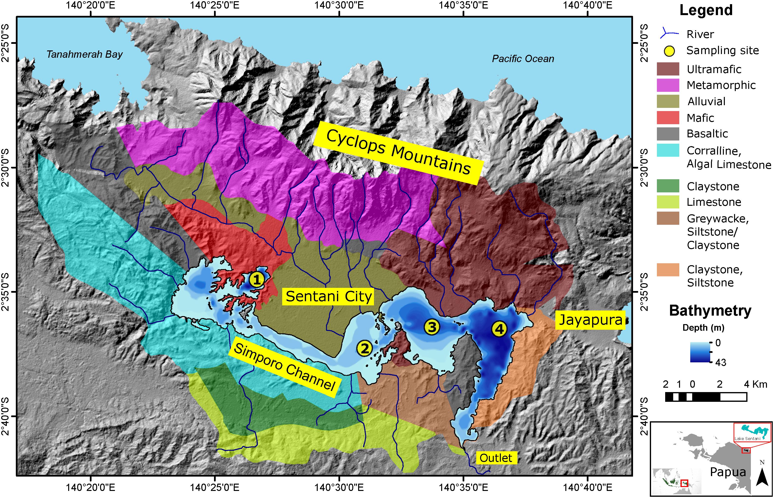
Figure 1. Map of Lake Sentani and its surrounding watershed. Catchment lithology is indicated by different colors. The lake is bounded by the Cyclops Mountains to the north and lowlands to the south. Sampling locations 1–4 are indicated by yellow circles. Locations 1 and 4 are located in the deepest sub-basins, whereas location 2 is in the shallowest sub-basin. The bathymetric map is modified after Sadi (2014), the lithology of Lake Sentani’s catchment is modified after Suwarna and Noya (1995) and the catchment boundary is modified after Sartimbul et al. (2015).
The lake has a catchment area of about 600 km2 and is bounded by the Cyclops Mountains (also called Cyclops Mountains) to the north (Tappin, 2007) and lowlands to the south. The north side of the lake is dominated by volcanic breccia, mafic, and ultramafic rocks as well as alluvial deposits, whereas the southern part of the lake is dominated by coralline-algal limestone, calcirudite, calcarenite of the Jayapura formation; sandstone and claystone, intercalation of limestone, siltstone and marl of the Aurimi formation; alluvial and basaltic deposits; alternating greywacke, siltstone and claystone intercalated with marl and conglomerate of the Makat formation; and finally Unk formation, consisting of alternating greywacke, claystone, siltstone, marl, conglomerate, and sandstone with lignite intercalations (Figure 1, Suwarna and Noya, 1995).
At least sixteen rivers drain into the lake. Yahim, the largest sub-catchment located on the north side of the lake, covers almost 38% of the total catchment (Supplementary Table 1). Twelve rivers come from the Cyclops Mountains on the northern side of the lake, and four rivers originate from the lowlands in the south (Figure 1). The Doyo River in the Yahim sub-catchment is the biggest single source of water to the lake with an average discharge of 18.98 m3s–1 (Supplementary Table 1, Handoko et al., 2014). The other rivers have discharge rates of <1 m3s–1; many are ephemeral and only have water during the wet season. The Jayafuri (also Jaifuri or Jayefuri) River, located in the southeastern tip of the easternmost basin, is the only outlet, having a discharge rate of 15.66 m3s–1 (Kementerian Lingkungan Hidup Republik Indonesia, 2011; Handoko et al., 2014).
The average annual precipitation around Lake Sentani is 1,691 mm/year (Sartimbul et al., 2015). Highest precipitation occurs in March, with an average of 206 mm; July has the lowest precipitation with 95 mm. Air temperature around Lake Sentani ranges between 23.6 and 32.2°C with July being the coldest month. Water temperature ranges from 29.3 to 30.5°C (Sadi, 2014). Lake Sentani shows significant heterogeneity with respect to spatial distribution of major elements in its surface sediment (Nomosatryo et al., submitted). The geochemical composition in the eastern basin of the lake is dominated by siliciclastic minerals, whereas the western part is strongly influenced by mafic and ultramafic catchment lithology.
Materials and Methods
Field Campaigns
Three expeditions were carried out in April–May 2016, November 2016, and January 2018. Small local fishing boats were used as platforms. During the first campaign, we took measurements and samples at all four locations described in Figure 1. We sampled one location in the center and/or the deepest part of each sub-basin, locations were labeled 1–4 from west to east. Locations 1 and 4 have the greatest water depth and meromictic conditions. We measured the water depths at our sampling locations by echosounder, as well as by wireline. During the second campaign, we re-visited locations 2–4, and on the third campaign, we focused on the two sites with the deepest water and re-sampled location 1 in the westernmost sub-basin and measured profiles for water temperature, Dissolved Oxygen (DO), and conductivity at location 4 in the easternmost sub-basin.
Limnological Characterization and Water Column Sampling
During the first and third expedition, we measured profiles for water temperature, DO, and conductivity, using a conductivity-temperature-depth probe (CTD; Rinko-Profiler ASTD 102). During the second campaign in November 2016 we measured the same variables with a Water Quality data logger (YSI 6920, Yellow Springs Instruments, Yellow Springs, OH, United States). On all expeditions, measurements were also conducted on discrete water samples at 5- or 10-m depth resolution using a 5-L Niskin water sampler (General Oceanics, Miami, FL, United States). Water temperature, pH and conductivity were determined with a multi-parameter instrument (WTW, Multi 3420, Xylem Analytics, Germany); Dissolved Oxygen was measured with an optical Dissolved Oxygen Meter (YSI Pro ODO, Yellow Spring Instruments, Yellow Springs, OH, United States). Density of the water column was calculated from temperature profiles using R-package rLakeAnalyzer (Read et al., 2011).
Sediment and Pore Water Sampling
Sampling was conducted using a gravity corer (90 cm long, Ø 7 cm) and great care was taken to retrieve cores with an undisturbed sediment-water interface (SWI). We usually recovered duplicate sediment cores of at least 50 cm length from each sampling site. The cores were sectioned at 2-cm resolution from 0 to 20 cm depth, 5-cm resolution from 20 to 50 cm depth and 10-cm intervals below 50 cm. At least 16 depth intervals were collected from each core.
One entire core was sampled for pore water, another one for sediment analyses. Pore water sampling was conducted on site by squeezing with a small air-powered pore water press (Pore-water pressing bench, KC Denmark a/s). For each depth interval, at least 10 mL of pore water were collected in syringes, filtered through 0.2-μm pore size cellulose acetate membrane syringe filters to remove all particles and most microorganisms, transferred into 2-mL twist-top vials and stored at +4°C until analysis. Hydrogen Sulfide (HS–) in pore water was preserved by adding 0.4 ml of saturated ZnCl2 solution to 2 mL of sample.
Each sediment sample was packed into a gas-tight Aluminum foil bag and heat-sealed. Due to the unavailability of nitrogen gas, we tried to squeeze out as much air as possible, but some oxidation during storage and transport cannot be ruled out.
Water Analyses
Anion Analysis
Major inorganic anions (NO2–, PO43–, NO3–, and SO42–) were analyzed by using suppressed ion chromatography (IC). The system consisted of a SeQuant SAMS anion IC suppressor (EMD Millipore, Billerica, MA, United States), a S5200 sample injector, a 3.0 × 250 mm lithocholic acid column (LCA 14) and a S3115 conductivity detector (all Sykam, Fürstenfeldbruck, Germany). The eluent was 5 mM Na2CO3 with 20 mg L–1 4-hydroxybenzonitrile and 0.2% methanol. Flow rate was set to 1 mL min–1 and column oven temperature to 50°C. A multi-element anion standard (Sykam, Lot 20150220) containing NO2– (434.7 μM), PO43– (210.6 μM), NO3– (806.4 μM), and SO42– (520.5 μM) was diluted 10 times and measured every 10 samples along with a blank. Respective minimum detection (S/N = 3) and quantification limits (S/N = 10) were as follows: NO2– (4.1 μM; 14.14 μM), NO3– (2.8 μM; 9.3 μM), PO43– (4.3 μM; 14.3 μM) and SO42– (2 μM; 8.4 μM).
Cation Analysis
Major cations (Mg2+, Ca2+, and NH4+) were analyzed by using non-suppressed ion chromatography (IC). The IC system consisted of an S5300 sample injector (Sykam), a 4.6 × 200 mm Reprosil CAT column (Dr. Maisch HPLC, Ammerbuch-Entringen, Germany) and an S3115 conductivity detector (Sykam). The eluent was 175 mg L–1 18-Crown-6 and 120 μL L–1 methanesulfonic acid. The flow rate was set at 1.2 mL min–1 and column oven temperature at 30°C. A Cation Multi-Element Standard (Carl Roth) was diluted five times for calibration. Based on a respective signal-to-noise (S/N) ratio of 3 and 10 the detection and quantification limits were calculated for each ion and are as follows: Mg2+ (9.6 μM; 31.7 μM), Ca2+ (8.3 μM; 26.5 μM) and NH4+ (11.3 μM; 67.6 μM).
We also measured iron speciation on samples collected during the third expedition at location 1. The samples were kept in glass vials without headspace and measured photometrically (Viollier et al., 2000) within 6 h after sampling.
Phosphate Analysis
In most samples phosphate concentrations were below the detection limit of ion chromatography and were thus measured by spectrophotometry (Murphy and Riley, 1962). 0.5 mL sample was transferred to 1.5 mL disposable cuvettes (Brand Gmbh, Germany) and 80 μL reagent. The reagent was prepared by mixing 125 ml of 5 N sulfuric acid and 37.5 ml of 0.032 M ammonium molybdate, 75 ml of 0.1 M ascorbic acid solution and 12.5 ml of 4 mM potassium antimonyl tartrate solution. The absorbance was measured at 882 nm with a DR 3900 spectrophotometer (Hach, Düsseldorf, Germany). The detection limit of the method is 0.005 μM.
Sulfide Analysis
Hydrogen sulfide was preserved by adding 0.4 ml of saturated ZnCl2 solution to 2 mL of sample almost immediately after collection. The concentration of HS– was quantified spectrophotometrically using the methylene blue technique (Cline, 1969). Samples were measured by adding 40 μL diamine reagent to 0.5 mL homogenized ZnCl2-preserved samples. Absorption was measured at 668 nm using a DR 3900 spectrophotometer (Hach, Düsseldorf, Germany). The detection limit is 0.25 μM with a 1 cm cuvette. Samples were measured in duplicate. For all spectrophotometric analyses, the concentrations are given as average values; error bars are one standard deviation. Reproducibility was always better than 5%.
Total Alkalinity Determination and Dissolved Inorganic Carbon (DIC) Calculation
Total alkalinity (TA) was determined immediately after pore water squeezing by colorimetric titration, pH was measured using a Horiba pH-22 Twin Compact pH Meter. These two variables were used to calculate DIC from the carbonate speciation (DIC = CO2 + HCO3– + CO32–) using the LLNL method in PHREEQC (Parkhurst and Appelo, 1999).
Sediment Analyses
The sediment samples were freeze-dried and the large material such as rock, shells, twigs, and leaves, was removed using tweezers. Grinding was done manually in a porcelain mortar and the entire sediment sample was passed through a 63-μm-mesh sieve.
TC, TOC, and TN Analyses
For quantification of TC and TN, about 5 mg of material was combusted in tin foil at 950°C in a Vario EL III analyzer (Elementar Analysensysteme GmbH). For TOC quantification, about 15–100 mg of material was combusted at 580°C using a Vario Max C analyzer (Elementar Analysensysteme GmbH), after pretreatment with HCl. The detection limit of these methods was 0.1 wt.% for TOC and TN and 0.05% for TC.
Mineralogical Analyses
Mineralogical data were collected with a PANalytical Empyrean X-ray diffractometer operating with Bragg-Brentano geometry at 40 mA, 40 kV, and Cu-Kα radiation. A random distribution of the powdered sample was prepared for bulk-rock mineralogy analysis. The identification of the mineralogy was performed using the EVA 11.rev.0 Software (Bruker).
X-Ray Fluorescence (XRF) Scanning
About 4 g of freeze-dried sediment powder was loosely packed in sampling cups (∼2 cm high, Ø 2 cm) and covered with X-Ray-transparent foil. Analysis of elemental sediment composition was performed on these samples using an ITRAX XRF core scanner with a Cr X-ray source (30 kv, 55 mA, and 10 s). Element intensities of all samples (N = 55) obtained by XRF core scanning were calibrated using quantitative results of 11 discrete reference samples. Reference analyses were performed on glass beads using a PANalytical AXIOS Advanced XRF. International and internal reference samples were used for calibration. Coefficients of determination (R2) of the XRF scanning calibration are in Supplementary Table 1. Sediment characterization based on geochemical results was conducted using principal component analyses (PCA) and hierarchical clustering of the calibrated and log-ratio-transformed XRF core scanning data (Weltje et al., 2015). Element correlations and compositional grouping by means of hierarchical clustering were visualized using a biplot of the first two principal components.
Reaction Rate and Flux Calculations
Using the MatLab routine of Wang et al. (2008) we quantified net rates of production and consumption of several dissolved pore water compounds that play a quantitatively significant role in carbon remineralization processes. The model requires several data a priori. We used sediment porosity data from location 1 to calculate the reaction rates at all locations (Supplementary Table 3). Diffusion coefficients (assuming 25°C) of the respective compounds were 1.85 × 10⁻⁹ m2 s–1 for NH4+, and 1.11 × 10⁻⁹ m2 s–1 for HCO3– (Schulz, 2000). We used the latter as the dominant species of dissolved inorganic carbon (DIC). Because we did not have values for sedimentation rates at Lake Sentani, we used a typical value for tropical oligotrophic lakes (1.9 × 10⁻⁴ m yr–1, Russell et al., 2014) and assumed steady-state conditions. A minimum of five measured concentration data points was used to determine each reaction zone. Uncertainties in the rate estimates were quantified using a Monte Carlo technique (Wang et al., 2008).
Results
Water Column Characteristics
There were differences in the vertical structure of the water column among the locations and sampling times (Figure 2). At all four locations, temperatures ranged from 31.0 to 32.5°C at the lake surface to 29.0–30.0°C at the bottom, but each location exhibited a distinct temperature profile.
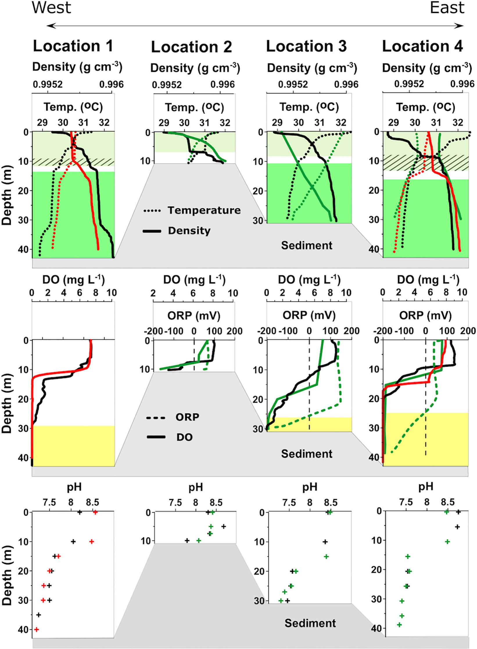
Figure 2. Water column profiles of density, temperature, dissolved oxygen (DO), oxidation-reduction potential (ORP), and pH of the four sampling locations in Lake Sentani. Measurements were taken in April (black) and November (green) 2016 and January 2018 (red). The profiles show clear thermal stratification with a well-mixed epilimnion extending to about 10 m water depth (light green shading) and a denser hypolimnion below about 15–20 m (dark green shading), depending on the basin and time of measurement. Diagonal line pattern indicates the fluctuations of the epilimnion boundary. Negative ORP values characterize the monimolimnion (yellow shading) with reducing conditions.
Both the temperature and density profiles show small but measurable fluctuations between seasons. Except for the measurements from the November 2016 campaign, when temperatures decreased rather steadily with depth, profiles from all other sites show a relatively distinct thermocline. The temperature profiles are mirrored by the density profiles, with lower values of 0.995 g cm–3 at the surface and 0.996 g cm–3 at the bottom. Temperature and density fluctuations have little effect on the depth of the oxycline, which appears to remain fairly stable throughout the year.
The two deepest locations, 1 and 4, show relatively steep oxyclines, with oxygen concentrations decreasing rapidly below 10 m water depth. The shallowest location (2) exhibits features similar to locations 1 and 4, although oxygen is never fully depleted because of the shallow water depth. At location 3 the decline in DO is much more gradual than at the other locations and only reaches full depletion at 25–30 m, similar to location 1. The depth of DO depletion marks the change of the Oxidation Reduction Potential (ORP) value from positive to negative.
At all locations, the surface water is slightly alkaline, with pH values around 8.5, dropping with depth by about one unit. The depth profiles are similar to the oxygen profile with a rapid decrease at the oxycline and a more gradual drop below. One notable feature of location 1 is that pH varies by about half a pH unit between April and November in the upper 10 m but remains stable at the other sites.
Anion and Cation Distributions in the Water Column and Porewater
The concentration profiles of dissolved anions and cations such as phosphate (PO43–), sulfate (SO42–), sulfide (HS–), ammonium (NH4+), Calcium (Ca), and Magnesium (Mg) in the water column and porewater are presented in Figure 3. Concentrations of NO3 and NO2 were below the detection limit in both the water column and pore water.
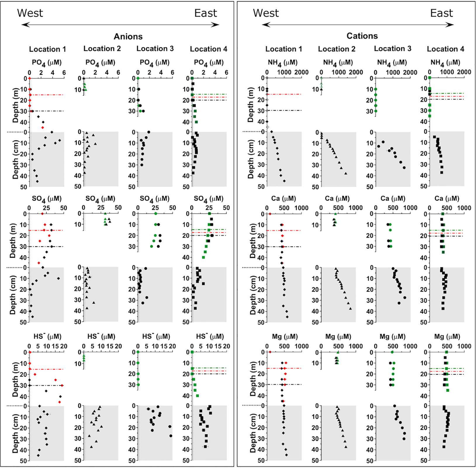
Figure 3. Vertical distribution of anions and cations in the Lake Sentani water column and sediment pore water. The horizontal dashed-dotted black lines indicate the oxycline on the different sampling dates, black indicates April 2016, green November 2016, and red January 2018. Pore water profiles are indicated by the gray shaded area. Reproducibility was always better than 5%. See main text for details.
At all four locations, phosphate concentrations in the oxic surface water were around our detection limit and only increased below the oxycline. At location 1 the depth of oxygen depletion had shifted from 15 to 30 m between the two sampling campaigns, but the phosphate profiles from both campaigns are identical. Despite some scatter in the data from locations 2 and 4, there appears to be a flux of dissolved phosphate out of the sediment into the water column at all locations.
Sulfate concentrations are 28–31 μM in the oxic surface water of all locations. Above the oxycline, values remain rather stable, but decrease in the anoxic part with concentrations between 10 and 15 μM at the SWI. Pore water sulfate concentrations decrease even further and fall below our detection limit (∼2 μM) in the upper few cm. Values remain around the detection limit throughout the rest of the core at all locations.
Hydrogen sulfide (HS–) concentrations in the oxic surface waters are below our detection limit at all locations, but increase with depth below the oxycline. There is a distinct difference between the concentration profiles below the oxycline at locations 1 and 4. Whereas the concave upward profile at location 1 indicates hydrogen sulfide production in the water column, the linear to the slightly concave downward profile at location 4 indicates no production in the water column but either a purely diffusive flux or consumption of hydrogen sulfide. Location 2 has a fully oxygenated water column and therefore no hydrogen sulfide. At location 3 the sample resolution below the oxycline is too low to asses whether any production or consumption takes place in the bottom water.
At location 1 the ammonium (NH4+) concentration profile in the water column shows low concentrations and a slight increase close to the SWI. However, it displays a different trend in the porewater. Generally, the concentration of NH4+ in the pore water increases with depth. Locations 2 and 3 have steeper pore water gradients than the other locations. Location 4 shows the lowest gradient.
Calcium and Magnesium concentrations in the water column reveal constant profiles from the surface to the bottom at all locations. In the porewater, there are two pairs of locations that display similar profiles; at locations 1 and 4 the relatively constant values from the water column continue, whereas at locations 2 and 3 the Ca2+ concentration profiles start to increase with depth below ∼10 cm depth in the sediment.
Reaction Rate of Organic Matter Mineralization
Production and consumption of dissolved pore water constituents can provide crucial information about early diagenetic reactions, most of which are driven by microbial activity. As organic matter mineralization leads to CO2 production, the DIC concentration can be used as a good proxy for microbial activity (Figure 4). At all locations, DIC concentrations increase with depth, although with different slopes. Locations 1 and 2 have almost linear gradients and only show curvature, i.e., production, in the upper 12 cm, whereas locations 3 and 4 show stronger curvature and higher DIC production rates.
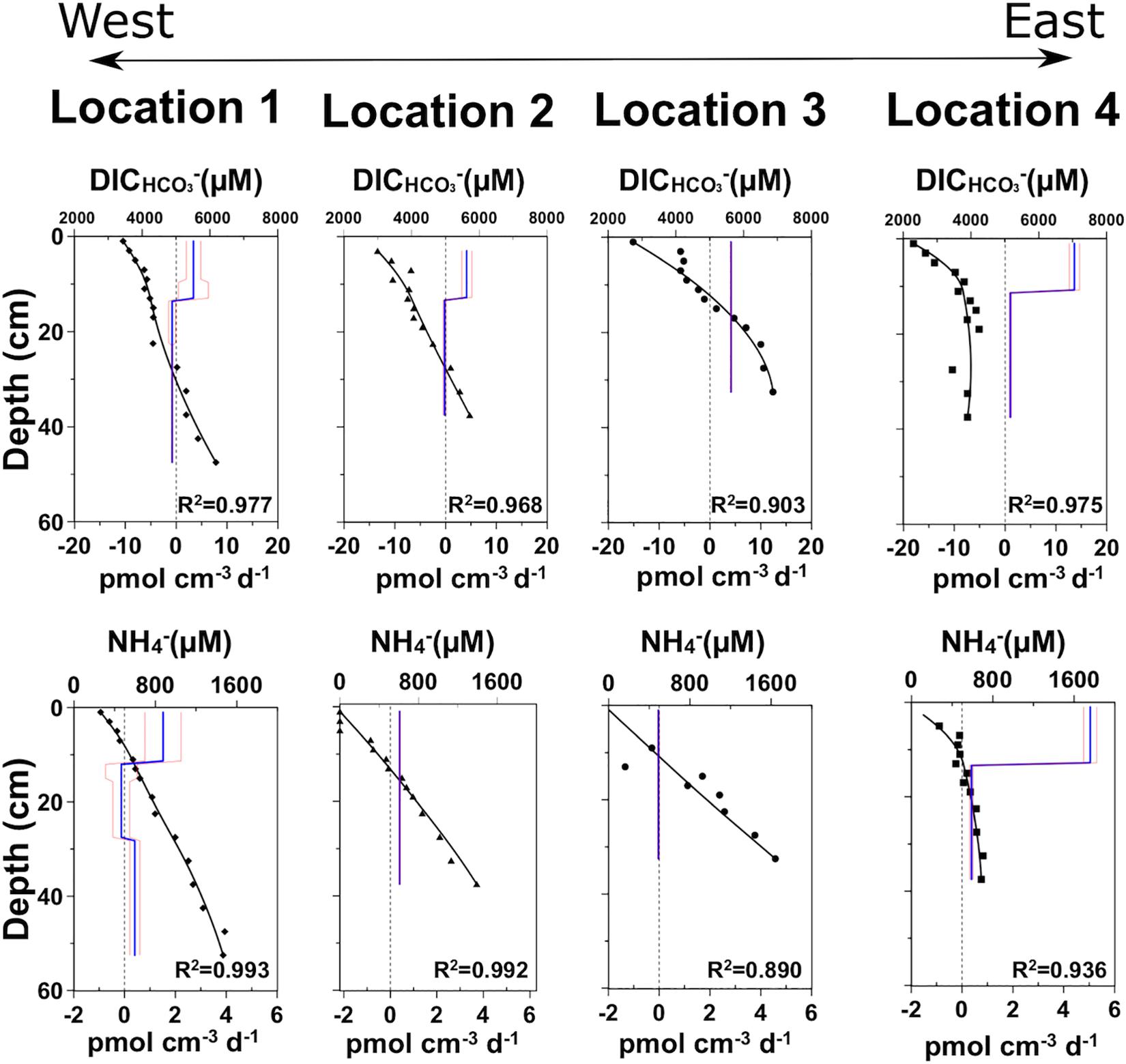
Figure 4. Calculated reaction rates based on measured pore water concentrations and physical properties. The symbols represent measured concentrations, the black line shows the modeled concentration. Production and consumption rates of the respective compound are shown by positive or negative values of the blue line, respectively. The red lines indicate error ranges. See main text for details.
Mineralization of organic matter also releases NH4+ to the porewater. As for DIC, concentrations increase with depth, but the respective profiles show somewhat different curvatures and hence zones of production. Locations 1 to 4 all show almost linear gradients, reflecting low production rates. Location 4 reveals a steeper slope in the NH4+ concentration profile, especially in the upper 15 cm, and consequently several times higher production rates.
Sediment Characteristics
Sediment Carbon and Nitrogen
With values between 8 and 16 dry wt% total carbon (TC), concentrations are dominated by organic carbon, which constitutes at least 80% of the TC (Figure 5). Surprisingly, the concentrations of TOC do not decrease with depth as a consequence of microbial degradation taking place continuously throughout the sediment column, but rather increase at all locations except location 1, which shows considerable scatter in the profile.
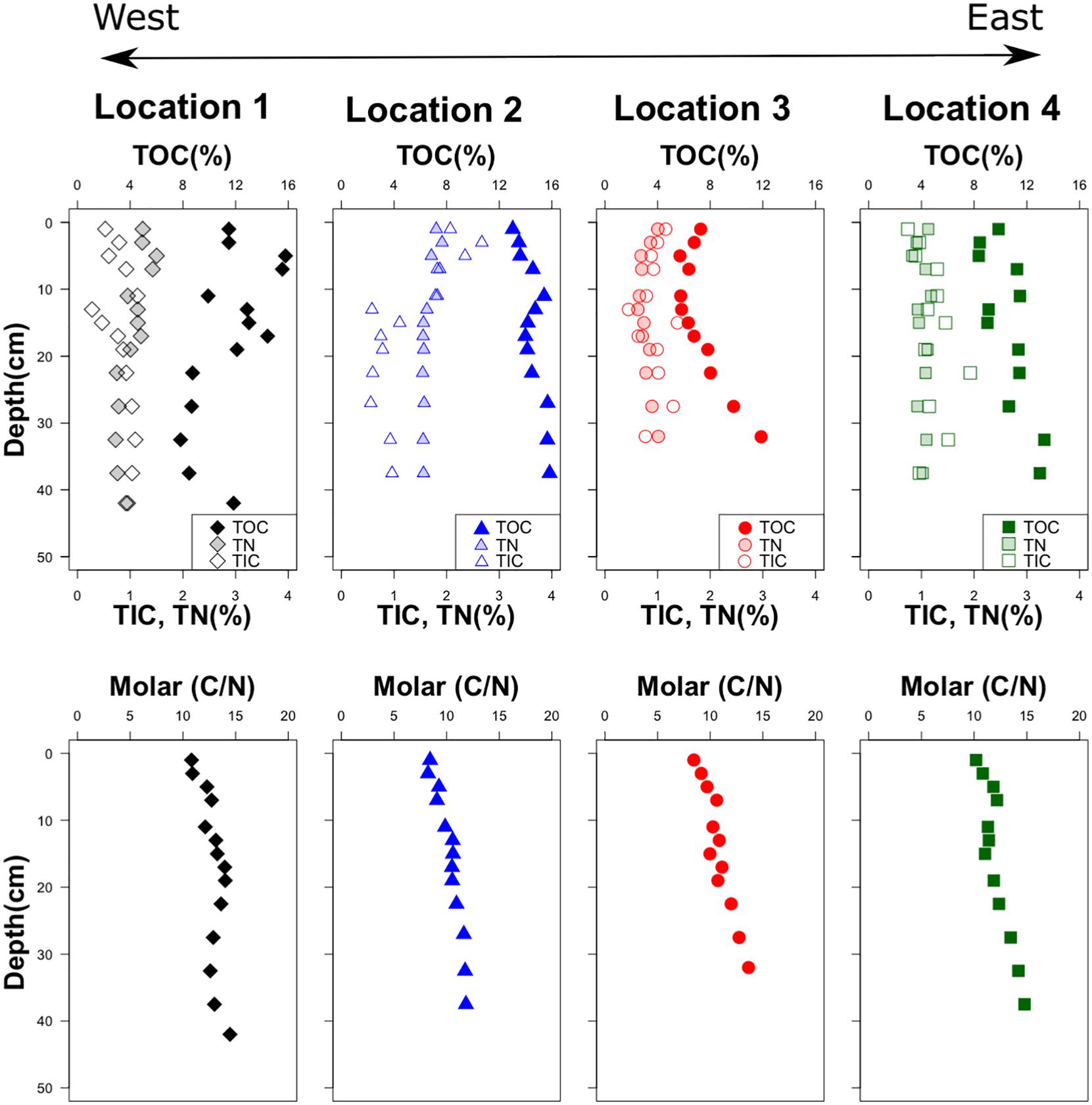
Figure 5. Down-core variation of total organic carbon (TOC), total inorganic carbon (TIC), total nitrogen (TN), and molar C/N ratio.
Total nitrogen (TN) concentrations are between 0.33 and 1.91%. With the exception of location 3, the concentration profiles are more or less constant with depth. The C/N ratios are very similar at all sites and depths, starting at the SWI with values around 8–10 and increasing more or less linearly to values close to 15 deeper in the profiles.
Mineralogy
The overall mineralogy in the samples is quartz, chlorite, kaolinite, plagioclase, pyrite, illite, and amphibole (Figure 6A). Based on the peak shape, chlorite-smectite interlayers were detected at locations 1 and 2, whereas dolomite was observed solely at location 1. Calcite is absent in all samples. Pyrite is more dominant in locations 1 and 2. These two locations also have higher sulfur and TOC values. Locations 3 and 4 contain a higher amount of ultramafic minerals such as amphibole and talc, originating from the Cyclops Mountains, whereas locations 1 and 2 contain material originating from catchment areas composed of alluvial, claystone, siltstone, sandstone, and carbonate rocks.
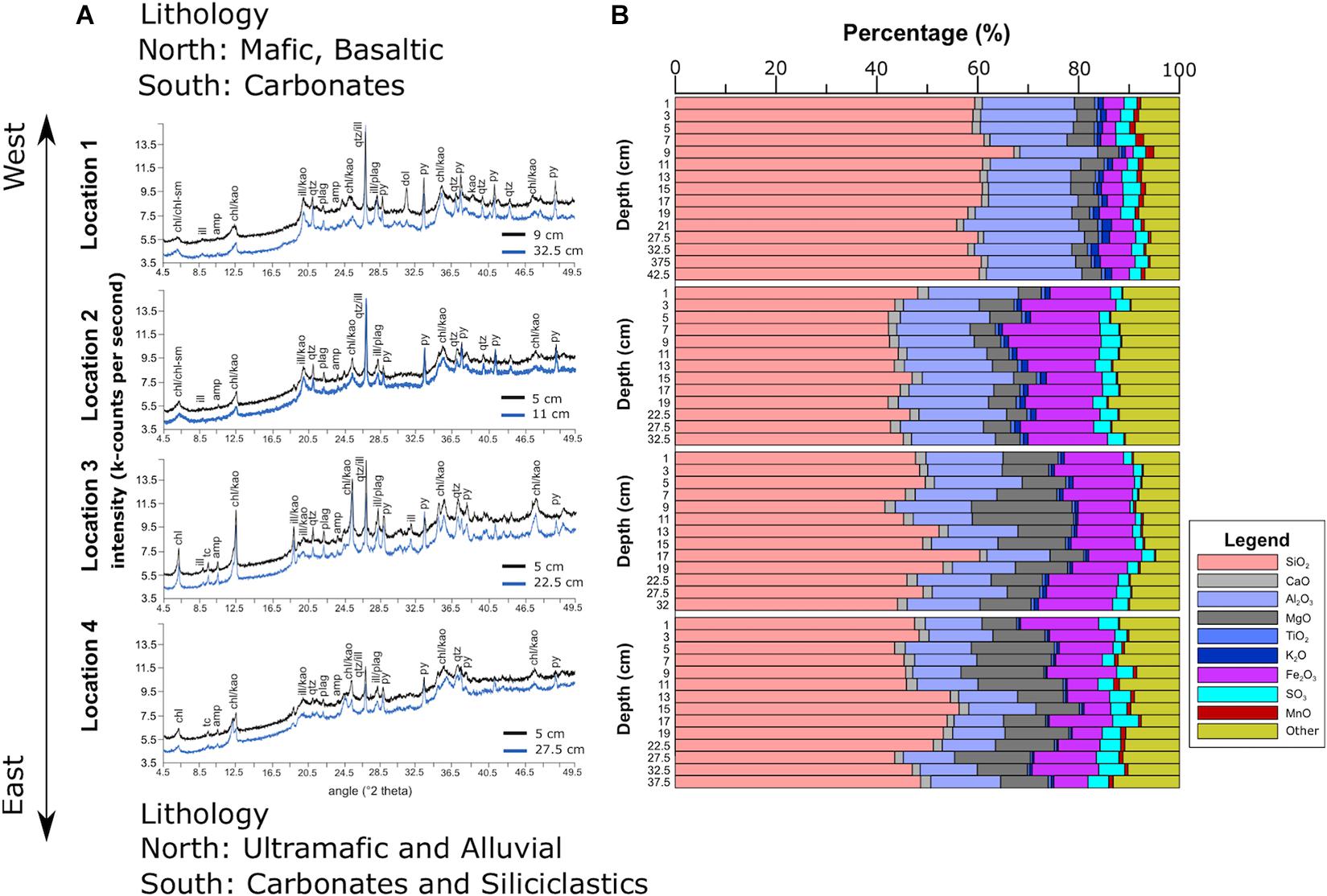
Figure 6. Mineralogy (A) and elemental composition (B) of Lake Sentani sediment. The term “Other” in (B) denotes other elements and organic matter.
Elemental Composition
Calibration results of the XRF core scanning data for major elements detected in Lake Sentani sediment include Mg, Al, Si, S, K, Ca, Ti, Mn, and Fe (Supplementary Tables 2, 4). The coefficients of determination (R2) of the calibration results are between 0.68 and 0.93, except for Ca (R2 = 0.09). The poor correlation of Ca can be ascribed to the low and very limited variations of the Ca concentrations in the samples, which range from 1.4 to 2.1% (Supplementary Tables 2, 4). Silica is the most abundant element and accounts for about 42–60 wt% at all locations. Location 1 shows higher Si concentrations than the others (Figure 6B). Ca is distributed almost evenly across all locations. Concentrations of Al and Mg show considerable differences between locations. With average concentrations of 18.37 and 16.67%, respectively, locations 1 and 2 have higher Al concentrations than locations 3 and 4. Magnesium shows the opposite pattern with average concentrations of 3.99 and 5.15% for locations 1 and 2, respectively, compared to 11.41 and 12.15% for locations 3 and 4. Iron concentration shows little variability within cores, but considerable differences between sites, with average concentrations of 4.1, 14.93, 12.53, and 9.89% at locations 1–4, respectively. Although Mn only accounts for a few percent of the total sediment, it shows a clear bimodal distribution, with higher values at locations 1 and 4 and lower ones at locations 2 and 3. Even though K and Ti only account for a maximum of one percent, K shows a gradual decrease from location 1 to location 4. The average concentration of Ti at location 1 is higher than at the other locations.
Sediment Geochemical Characteristics
The first two principal components PC1 and PC2 explain 47.1 and 29.1% of the total variance, respectively. The lithogenic elements Al, K, and Ti have a strong negative loading on PC1 and are oriented in the same direction indicating a positive correlation (Figure 7). The element Si shows a negative loading on PC1, but a positive loading on PC2. The element Si has two main sources, one is silicate frustules of diatoms and the other is siliciclastic minerals of the lithogenic sediment fraction. The elements Mg, Ca, and Fe all have a positive loading on PC1, but only Ca and Fe are oriented in the same direction indicating a positive correlation (Figure 7). The opposite orientation of lithogenic elements Al, K, Ti, and the elements Mg, Ca, and Fe along PC 1 reveals that these elements represent different sediment fractions that are negatively correlated.
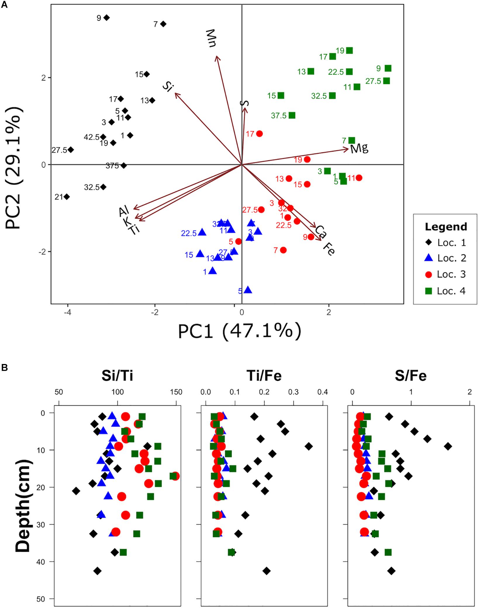
Figure 7. Principal Component Analysis (PCA) of the elemental composition (A) and ratios of selected elements (B). Both the first and second Principal Component (PC) contribute to distinguishing sediment characteristics between locations. The selection of elements for the ratios was based on the fact that each pair is on opposite ends of one of the PCA axes. The numbers in (A) indicate sediment depth (cm).
The four sediment cores can be clearly distinguished based on their distribution in the PCA biplot (Figure 7A). Samples from location 1 all group on the left side of the biplot, whereas locations 2–4 group on the right and display a gradual and partly overlapping shift with respect to PC2. The distribution of the four locations suggests that lithogenic sediments are more dominant at locations 1 and 2, with a stronger influence of Si at location 1 and Al, K and Ti at location 2. The gradual change displayed by locations 2–4 suggests an increasing influence of the elements Mn and S, which is probably related with an increasing amount of organic matter.
PC2 has an opposite correlation of the two redox-sensitive elements Mn and Fe. In both locations 1 and 4, there is a weak correlation between PC2 and sediment depth. Although location 1 shows decreasing PC2 values with increasing depth, with the three deepest samples revealing negative numbers, location 4 shows the opposite trend, with the three shallowest samples having negative PC2 values.
Based on the PCA analysis, we found that Ti forms opposing pairs with Fe and Si on PC1 and PC2, respectively. A similar pair is formed by S and Fe on PC2. Therefore, these element ratios (Figure 7B) can be used as proxies for different sediment input and water column conditions.
Discussion
Physicochemical Characteristics of the Water Column
The water column profiles show clear signs of stratification, which have profound effects on the overall structure of the water column and bottom water oxygenation in all four sub-basins of Lake Sentani. Although all sub-basins have a well-mixed epilimnion, basins 1 and 4 both have anoxic monimolimnia (Figure 2), and in basin 3, DO just reaches depletion at the SWI and basin 2 remains oxic, albeit at low concentrations (Figure 2). These findings indicate that there is one location that is oxygenated (2), one intermediate (3) and two fully meromictic basins (1 and 4) in Lake Sentani, while all four sub-basins share the same surface water chemistry. We did not sample in the coldest month (June), when overturn would be most likely, but the water column profiles from the other three sampling campaigns show relatively little variation, so we are confident that the water column is stable throughout the year.
Different patterns of water column stratification are reflected in the pore water profiles. The vertical distribution patterns of anions differ considerably between the fully oxygenated (loc. 2), the intermediate basin (loc. 3) and the two meromictic basins (loc. 1 and 4). Even in highly oligotrophic lake systems with low sediment organic carbon concentrations and fully oxygenated bottom waters, oxygen penetrates at most only a few mm into the sediment (Corzo et al., 2018). Therefore, reducing conditions and hence anaerobic processes are prevalent in the sediment at all locations (Figure 3).
In the absence of other electron acceptors with a higher energy yield (NO32–, Fe3+, and Mn4+), the anaerobic degradation of organic matter will proceed via sulfate reduction (Froelich et al., 1979). Sulfate concentrations in Lake Sentani are around 18–25 μM, which is about twice as high as in other oligotrophic lakes in Indonesia, e.g., Lake Matano or Lake Towuti, but less than one thousandth that in the ocean (Jørgensen et al., 2001; Vuillemin et al., 2016). Sulfate concentrations are more or less constant throughout the water column of the oxic basin (loc. 2) and above the oxycline in the meromictic basins (loc. 1 and 4). The product of sulfate reduction, HS–, is present in all sediment samples at all locations, but the considerable scatter within the profiles, possibly indicating some degree of sulfide oxidation during sample handling, prevents the identification of clear depth trends. Nevertheless, the presence of HS– indicates that even such low sulfate concentrations are sufficient to enable microbial sulfate reduction (Crowe et al., 2014; Vuillemin et al., 2016).
Although it is not surprising that there is no HS– in the oxic water column of location 2, even the low DO concentrations at the SWI of loc. 3 appear to be sufficient to facilitate oxidation of HS–. At locations 1 and 4, HS– is present throughout the monimolimnion and only becomes depleted at the oxycline. Unfortunately, the data show too much scatter (loc. 1) and have insufficient resolution (loc. 4) to assess whether the HS– concentration profile is purely diffusive and sulfide oxidation is limited to the oxycline or whether it indicates production or consumption throughout the monimolimnion. It is interesting to note that sulfate and sulfide coexist in the monimolimnia of locations 1 and 4. Given the thermodynamically constrained sequence of electron acceptor use (Froelich et al., 1979), there appear to be sufficient available electron donors that would yield greater energy than sulfate. In this case nitrate and manganese oxides are not quantitatively important, and ferric iron is most probably the main electron donor (Supplementary Figure 1) thereby preventing sulfate reduction. We consider neither anoxygenic photosynthesis nor sulfide oxidation with another electron acceptor to be a significant source of sulfate in the monimolimnion. There are no suitable electron acceptors available and anoxygenic photosynthesis can be excluded due to water depth. Moreover, the concentration profiles of sulfate and sulfide provide no indication for sulfide oxidation.
Despite some variation in maximum concentration levels, the PO43– profiles are quite similar at all locations. Similar to HS–, the shape of the concentration profiles in the water column reflects redox conditions, with both ions only showing enrichment in the sediment pore water and anoxic parts of the water column, indicating that the oxic-anoxic interface represents an efficient barrier for both ions, although the mechanisms that govern their respective concentrations are quite different. Whereas HS– can be oxidized both biologically and abiologically (Millero, 1991), PO43– is usually bound in biomass or adsorbed to mineral surfaces, particularly Fe-oxy-hydroxides (Davison, 1993).
The increasing concentration of phosphorus in the anoxic bottom water is apparently caused by release of iron-oxide-bound phosphate. Although we only have iron speciation data from location 1 (Supplementary Figure 2), they indicate that phosphate and iron are tightly coupled. Below the oxycline, the concomitant increase in dissolved PO4 and Fe (II) show that the reduction of solid Fe (III) to dissolved Fe (II) leads to a release of adsorbed PO4. The same process has also been shown for tropical ferruginous and oligotrophic Lake Matano, South Sulawesi, Indonesia (Crowe et al., 2008; Katsev et al., 2010).
The different patterns in ion distribution in relation to water column structure of each basin are clearly shown in the cation concentration profiles. The cation species analyzed in our study are not involved in redox processes, however, the anaerobic mineralization of organic matter will liberate ammonium as a product (Hansen and Blackburn, 1991; Beutel, 2006). Different from HS– and PO43–, which diffuse out of the sediment and become enriched in the anoxic water column, NH4+ mainly remains below our detection limit in most water column samples, except the bottom two samples of location 1 (Figure 3). Interestingly, the pore water NH4+ concentration profiles increase at a steeper rate in basins 2 and 3, which have oxygenated bottom waters, than in meromictic basins 1 and 4. We do not have an explanation for this observation, but one possibility could be the difference in N-incorporation efficiencies between aerobic and anaerobic bacteria (Hansen and Blackburn, 1991; Canfield et al., 1993).
As for ammonium, the concentration profiles of Ca and Mg, particularly the pore water profiles, can be divided into two groups, according to the stratification of the water column. Meromictic basins 1 and 4 reveal the same concentration throughout the water column and the sediment, indicating no net consumption (loss) or production (gain) of either compound on either side of the oxycline, although at location 4 there is a slight excursion to higher values in the upper 10 cm of the sediment. In basins 2 and 3 the water column profiles also do not show any concentration changes, but the sediment pore water concentration profiles continue the trend from the water column through the upper ∼10 cm before starting to increase almost linearly with depth; at 30 cm depth they reach values that are higher by about 50% than in the water column. The depth at which the concentrations of Ca and Mg increase starts coincides with the depth at which ammonium also starts to become enriched in the pore water. A possible explanation could be oxidation of sulfide minerals (FeS and FeS2, Figure 6A), which are present in the upper part of the sediment. Sulfide oxidation produces protons that could facilitate the dissolution of calcite and dolomite in the sediment (Smolders et al., 2006). However, the XRF analyses of the sediment do not indicate preferential dissolution of Ca and Mg at locations 2 and 3, and moreover we cannot identify potential oxidants that could drive this reaction.
Overall, the vertical concentration profiles indicate differences in biogeochemical processes between the basins. Although in meromictic basins 1 and 4, the bottom water and the sediment pore water are to some degree a single continuous system, even low DO concentrations are sufficient to form an effective barrier for reduced species.
Geochemical Characteristics
The geochemical composition of Lake Sentani’s surface sediment (Nomosatryo et al., submitted) and the short cores presented in this study is the result of equilibrium processes between the sediment, porewater and water column. The differences in sediment composition are representative of (i) the different processes and conditions in the water column of the basins, as well as (ii) the different sediment input caused by lithological variations in the catchment. The mafic and ultramafic lithology of the Cyclops Mountains deliver more Mg and Fe into basins 3 and 4 (Figures 1, 7). Since Al and Ti are not redox sensitive, they are relatively conservative during diagenetic processes (Boës et al., 2011) and therefore rather immobile. Fe and Mn are both highly redox sensitive and therefore strongly involved in redox-driven element cycling, particular in those basins where conditions become anoxic in the water column.
Weathering in the catchment area leaches elements such as Mg, Ca, Fe from the bedrock and soils, which are eventually transported into the lake via rivers, streams or mass wasting and direct runoff from the slope. The less soluble elements Al, Si, and Ti enter the lake as particulates rather than in dissolved form. Dissolved elements and particulates undergo biological and chemical transformation in the water column before deposition on the lake floor (Sheppard et al., 2019) where diagenetic processes further change the composition of the sediment (Davies et al., 2015; Rothwell and Croudace, 2015).
The distinct geochemical characteristics in sediment composition between the different locations are the result of several factors. The most important factor appears to be the lithology of the catchment. Lake Sentani is bounded to the north by the Cyclops Mountains, which are mainly composed of Fe- and Mg-rich mafic and ultramafic rocks. However, most of the runoff from these areas enters the two easternmost basins, 3 and 4, hence their correlation with Fe and Mg on PC1 (Figure 7). Nomosatryo et al. (submitted) showed that there is strong enrichment of Mn in the deepest part of basin 4, roughly coinciding with location 4 used in this study. In our present study we can show that the sediment cores from both deepest basins (1,4) reveal higher Mn concentrations than shallower basins 2 and 3. Consequently, locations 1 and 4 plot positively on PC2, and so does Mn (Figure 7). Although the ultimate reason for the enrichment could not be identified there are strong indications that the enrichment was caused by enhanced biogeochemical cycling of Mn, whereas the much more abundant Fe behaved more like a detrital element, which might also explain its correlation with Mg and Ca. At first glance it appears counterintuitive that sediment from location 1, which is surrounded by basaltic and mafic rocks has the lowest Fe concentrations. However, most rivers that enter basin 1 come from the west and the south and drain catchments mainly composed of limestone (Figure 1). Moreover, because these rivers are small and ephemeral (Supplementary Table 1), plus the fact that they are flowing through very flat terrain, and location 1 being rather well isolated from these rivers, it is not too surprising that Ca and Mg are low at this location as well. So it is not just the geology of the immediate surrounding that shapes the elemental and mineralogical composition of a lake sediment, but also the pathways of the rivers draining into it and the topography of the terrain.
Location 1 is a good example of the shifting geochemical composition over different time scales. The relatively small basin is subdivided by two peninsulas with steep slopes that reach deep into the basin. Location 1 seems to be weakly stratified as shown by the DO profile data, where the depth of the oxycline changed from 30 to 15 m between April 2016 and December 2018 (Figure 2). Water column dynamics also affect the concentration profiles of redox-sensitive anions like sulfate and sulfide. Compared to the other meromictic location 4, the profiles show more scatter, which we interpret as a result of non-steady-state conditions in response to a rapidly fluctuating oxycline depth. On longer timescales, we can also observe shifts in geochemical conditions caused by changes in sediment input. The PCA provides a weak indication for a change in sediment composition around a depth of 19 cm, and with one exception (42.5 cm) all samples below this depth have lower or even negative PC2 values. At this depth we can also observe a shift in TC, TN, and C/N ratio (Figure 5). As we do not have any age information from the sediment cores we can only speculate about the reason for this shift, but it clearly shows that each basin individually records local variations in sediment input or diagenesis, which might have multiple causes, e.g., changes in water column stratification, bottom water oxygenation, changes in land cover or runoff in the catchment. Identification of the reasons for these changes is beyond the scope of this study but our data show that these sediments offer the chance to study small-scale variations in the catchment and/or the water column.
Location 4 is also meromictic, but its stratification is much more stable than at location 1, given the little variation in oxycline depth over the different sampling campaigns. This results in more stable concentration gradients, showing less scatter and very little difference between the sampling campaigns. The sediment at this location also reveals compositional changes with depth. The three uppermost samples, from the SWI to 6 cm, are the only ones with a negative PC2 (Figure 7). These three samples also show a markedly different trend in TC and TN (Figure 5), indicating a shift in sedimentary input.
The differences in water column structure do not have a noticeable impact on the quality or the amount of sediment organic matter (OM). The fact that variations in sediment organic matter composition correlate with changes in element composition indicates that changes in environmental variables like erosion rates or land cover have a decisive influence on sediment composition. Although there are similarities in concentration profiles of individual elements and variables among basins, there is a sufficient number of differences that clearly show that each basin underwent its own evolution and its sediment provides a sensitive record of small-scale environmental variations.
The TOC concentration is influenced by both initial production and deposition of biomass and subsequent degradation (Meyers and Teranes, 2001). In all basins, TOC concentrations are sufficiently high to fuel abundant microbial respiration and therefore diagenetic processes. The concentrations lie between values typical for oligotrophic tropical lakes like Lake Towuti (2–3.5%) (Vuillemin et al., 2016) to eutrophic ones like Lake Maninjau (∼22%) (Henny and Nomosatryo, 2012). The source of organic matter appears to be relatively similar between locations, although there are local variations in both concentration and composition of organic matter, the latter being indicated by variable quantities of diatom frustules, found in smear slides (data not shown).
Even though nutrient concentrations in the water column are currently low, shifts in productivity are recorded in the sediment record. Overall the C/N ratio increases with depth, which can be interpreted either as a gradual shift from a more terrestrial organic matter input (with relatively higher C/N ratio) toward a lacustrine (phytoplankton) source of organic matter (Meyers, 2003). Another possibility could be increasing degradation of the more reactive algal material over time (Kaushal and Binford, 1999). Without any detailed analyses of the sediment organic matter, we are not able to provide a definitive explanation for the trend. We suspect that the higher C/N ratio in deeper sediment relates to past climate change but without proper age information this remains speculative.
The quantitatively dominant element in Lake Sentani is Si (Figure 6). Both biogenic (diatoms) and abiogenic Si (silisiclastics) are present in all samples although biogenic Si is never dominant. The opposite loading vector of Si and Ti on the PC2 (Figure 7) can be used as an indicator of the source of Si. High Si and low Ti indicate a more biogenic source, and low Si and high Ti a more abiogenic one. Given the small size of the individual basins and the many factors that influence element distribution in the sediment it remains questionable whether the Si/Ti ratio could be used to reconstruct productivity in the lake. The fact that both meromictic basins correlate positively with Si indicates that water column structure appears to have an influence on this ratio as well. Still, the correlation between sediment depth and PC2 for locations 1 and 4, albeit weak, can be interpreted as an indication of changing productivity over time.
Conclusion
Despite sharing a common surface water chemistry, each of the four sub-basins of Lake Sentani has a distinct water column structure and sediment chemistry. The effects of water column stratification and shifts in oxygenation levels appears to be most pronounced in the deeper basins. Sediment composition is mostly controlled by catchment geology, but water column stratification and in particular bottom water oxygenation has a strong influence on the elemental composition of the sediment and pore water composition. Depth profiles of dissolved chemical species in the water column and the sediment pore water provide information on fluxes, rates and hot spots of mainly microbially driven organic matter degradation processes. Lake Sentani provides a unique chance to study the influence of different environmental factors on sediment composition under identical climate and hydrological conditions.
Data Availability Statement
The original contributions presented in the study are included in the article/Supplementary Material, further inquiries can be directed to the corresponding author/s.
Author Contributions
SN, JK, and CH sampled in the field. PB and CH provided logistical support. SN, RT, and AS analyzed the samples. SN, RT, AS, and JK analyzed the data. SN wrote the manuscript with input from JK, DW, RT, and AS. All authors contributed to the article and approved the submitted version.
Funding
SN was financially supported by the Program for Research and Innovation in Science and Technology (RISET-Pro, World Bank Loan No. 8245-ID) – Ministry of Research, Technology.
Conflict of Interest
The authors declare that the research was conducted in the absence of any commercial or financial relationships that could be construed as a potential conflict of interest.
Acknowledgments
The authors thank Fauzan Ali (director of Research Center for Limnology-LIPI) for his support. Henderite Ohee (Cenderawasih University, Papua), and the late Herry Kopalit (University of Papua, Manokwari) managed field work. Axel Kitte is thanked for his invaluable assistance in the field and the lab, Brian Brademann and Nikolai Klitscher provided additional lab assistance and Dyke Scheidemann (AWI-Potsdam) helped with the TOC quantification.
Supplementary Material
The Supplementary Material for this article can be found online at: https://www.frontiersin.org/articles/10.3389/feart.2021.671642/full#supplementary-material
References
Beutel, M. W. (2006). Inhibition of ammonia release from anoxic profundal sediments in lakes using hypolimnetic oxygenation. Ecol. Eng. 28, 271–279. doi: 10.1016/j.ecoleng.2006.05.009
Boës, X., Rydberg, J., Martinez-Cortizas, A., Bindler, R., and Renberg, I. (2011). Evaluation of conservative lithogenic elements (Ti, Zr, Al, and Rb) to study anthropogenic element enrichments in lake sediments. J. Paleolimnol. 46, 75–87. doi: 10.1007/s10933-011-9515-z
Burdige, D. J., and Gieskes, J. M. (1983). A pore water/solid phase diagenetic model for manganese in marine sediments. Am. J. Sci. 283, 29–47. doi: 10.2475/ajs.283.1.29
Canfield, D. E., Thamdrup, B., and Hansen, J. W. (1993). The anaerobic degradation of organic matter in Danish coastal sediments: iron reduction, manganese reduction, and sulfate reduction. Geochim. Cosmochim. Acta 57, 3867–3883. doi: 10.1016/0016-7037(93)90340-3
Cline, J. J. D. (1969). Spectrophotometric determination of hydrogen sulfide in natural waters1. Limnol. Oceanogr. 14, 454–458. doi: 10.4319/lo.1969.14.3.0454
Corzo, A., Jiménez-Arias, J. L., Torres, E., García-Robledo, E., Lara, M., and Papaspyrou, S. (2018). Biogeochemical changes at the sediment-water interface during redox transitions in an acidic reservoir: exchange of protons, acidity and electron donors and acceptors. Biogeochemistry 139, 241–260. doi: 10.1007/s10533-018-0465-7
Crowe, S. A., O’Neill, A. H., Katsev, S., Hehanussa, P., Haffner, G. D., Sundby, B., et al. (2008). The biogeochemistry of tropical lakes: a case study from Lake Matano, Indonesia. Limnol. Oceanogr. 53, 319–331. doi: 10.4319/lo.2008.53.1.0319
Crowe, S. A., Paris, G., Katsev, S., Jones, C. A., Kim, S. T., Zerkle, A. L., et al. (2014). Sulfate was a trace constituent of Archean seawater. Science 346, 735–739. doi: 10.1126/science.1258966
Davies, S. J., Lamb, H. F., and Roberts, S. J. (2015). “Micro-XRF core scanning in palaeolimnology: recent developments” in Micro-XRF Studies of Sediment Cores. Developments in Paleoenvironmental Research, Vol. 17, eds I. Croudace and R. Rothwell (Dordrecht: Springer).
Davison, W. (1993). Iron and manganese in lakes. Earth Sci. Rev. 34, 119–163. doi: 10.1016/0012-8252(93)90029-7
Escobar, J., Serna, Y., Hoyos, N., Velez, M. I., and Correa-Metrio, A. (2020). Why we need more paleolimnology studies in the tropics. J. Paleolimnol. 64, 47–53. doi: 10.1007/s10933-020-00120-6
Feeley, K. J., and Stroud, J. T. (2018). Where on Earth are the “tropics”? Front. Biogeogr. 10, 1–7. doi: 10.21425/F5101-238649
Flemming, H. C. (1995). Sorption sites in biofilms. Water Sci. Technol. 32, 27–33. doi: 10.2166/wst.1995.0256
Froelich, P. N., Klinkhammer, G. P., Bender, M. L., Luedtke, N. A., Heath, G. R., Cullen, D., et al. (1979). Early oxidation of organic matter in pelagic sediments of the eastern equatorial Atlantic: suboxic diagenesis. Geochim. Cosmochim. Acta 43, 1075–1090. doi: 10.1016/0016-7037(79)90095-4
Handoko, U., Suryono, T., and Sadi, N. H. (2014). Karakteristik Fisiko-Kimia Sungai Inlet-Outlet Danau Sentani Papua. Prosiding Seminar Nasional Limnologi VII Tahun 2014. Gedung APCE, Cibinong Science Centre-Botanical Garden. Bogor: Pusat Penelitian Limnologi, Lembaga Ilmu Pengetahuan Indonesia, 226–236.
Hansen, L. S., and Blackburn, T. H. (1991). Aerobic and anaerobic mineralization of organic material in marine sediment microcosms. Mar. Ecol. Progr. Ser. 75, 283–291. doi: 10.3354/meps075283
Henny, C., and Nomosatryo, S. (2012). Dinamika sulfida di danau maninjau: implikasi terhadap pelepasan fosfat di lapisan hipolimnion. Limnotek 19, 102–112.
Indrayani, E., Nitimulyo, K. H., Hadisusanto, S., and Rustadi, R. (2015a). Analisis kandungan nitrogen, fosfor dan karbon organik di Danau Sentani - Papua. J. Manus. Dan Lingkungan 22, 217–225. doi: 10.22146/jml.18745
Indrayani, E., Nitimulyo, K. H., Hadisusanto, S., and Rustadi, R. (2015b). Peta batimetri Danau Sentani Papua. Depik 4, 116–120.
Jørgensen, B. B., Weber, A., and Zopfi, J. (2001). Sulfate reduction and anaerobic methane oxidation in Black sea sediments. Deep Sea Res. Part I Oceanogr. Res. Papers 48, 2097–2120. doi: 10.1016/s0967-0637(01)00007-3
Katsev, S., Crowe, S. A., Mucci, A., Sundby, B., Nomosatryo, S., Haffner, G. D., et al. (2010). Mixing and its effects on biogeochemistry in the persistently stratified, deep, tropical Lake Matano, Indonesia. Limnol. Oceanogr. 55, 763–776. doi: 10.4319/lo.2010.55.2.0763
Katsev, S., Verburg, P., Llirós, M., Minor, E. C., Kruger, B. R., and Li, J. (2017). “Tropical meromictic lakes: specifics of meromixis and case studies of Lakes Tanganyika, Malawi, and Matano,” in Ecology of Meromictic Lakes, eds R. D. Gulati, E. S. Zadereev, and A. G. Degermendzhi (Cham: Springer International Publishing), 277–323. doi: 10.1007/978-3-319-49143-1_10
Kaushal, S., and Binford, M. W. (1999). Relationship between C:N ratios of lake sediments, organic matter sources, and historical deforestation in Lake Pleasant, Massachusetts, USA. J. Paleolimnol. 22, 439–442.
Kementerian Lingkungan Hidup Republik Indonesia (2011). Profil 15 Danau Prioritas Nasional. Jakarta: Kementerian Lingkungan Hidup.
Konhauser, K. O., Fyfe, W. S., Ferris, F. G., and Beveridge, T. J. (1993). Metal sorption and mineral precipitation by bacteria in two Amazonian river systems: Rio Solimoþes and Rio Negro, Brazil. Geology 21, 1103–1106. doi: 10.1130/0091-7613(1993)021<1103:msampb>2.3.co;2
Lohman, D. J., de Bruyn, M., Page, T., von Rintelen, K., Hall, R., Ng, P. K. L., et al. (2011). Biogeography of the Indo-Australian Archipelago. Ann. Rev. Ecol. Evol. Syst. 42, 205–226. doi: 10.1146/annurev-ecolsys-102710-145001
Lukman, and Fauzi, H. (1991). Laporan Pra Survai Danau Sentani Irian Jaya dan Wilayah Sekitarnya. Pusat Penelitian Pengembangan Limnologi. Jakarta: Lembaga Ilmu Pengetahun Indonesia (LIPI).
Martin-Puertas, C., Tjallingii, R., Bloemsma, M., and Brauer, A. (2017). Varved sediment responses to early Holocene climate and environmental changes in Lake Meerfelder Maar (Germany) obtained from multivariate analyses of micro X-ray fluorescence core scanning data. J. Q. Sci. 32, 427–436. doi: 10.1002/jqs.2935
Meyers, P. A. (2003). Application of organic geochemistry to paleolimnological reconstruction: a summary of examples from the Laurention Great Lakes. Organic Geochem. 34, 261–289. doi: 10.1016/s0146-6380(02)00168-7
Meyers, P. A., and Teranes, J. L. (2001). “Sediment organic matter,” in Tracking Environmental Change Using Lake Sediments: Physical and Geochemical Methods, eds W. M. Last and J. P. Smol (Dordrecht: Springer), 239–269.
Millero, F. J. (1991). The oxidation of H2S in the Chesapeake Bay. Estuar. Coast. Shelf Sci. 33, 521–527.
Murphy, J., and Riley, J. P. (1962). A modified single solution method for the determination of phosphate in natural water. Anal. Chim. Acta 27, 31–36. doi: 10.1016/s0003-2670(00)88444-5
Parkhurst, D. L., and Appelo, C. A. J. (1999). User’s Guide to PHREEQC (version 2) – A Computer Program for Speciation, Batch-Reaction, One-Dimensional Transport, and Inverse Geochemical Calculations. Water-Resources Investigations Report 99-4259. Denver, CO: US Geological Survey.
Read, J. S., Hamilton, D. P., Jones, I. D., Muraoka, K., Winslow, L. A., Kroiss, R., et al. (2011). Derivation of lake mixing and stratification indices from high-resolution lake buoy data. Environ. Model. Softw. 26, 1325–1336. doi: 10.1016/j.envsoft.2011.05.006
Rothwell, R., and Croudace, I. (2015). “Micro-XRF studies of sediment cores: a perspective on capability and application in the environmental sciences,” in Micro-XRF Studies of Sediment Cores. Developments in Paleoenvironmental Research, Vol. 17, eds I. Croudace and R. Rothwell (Dordrecht: Springer).
Russell, J. M., Vogel, H., Konecky, B. L., Bijaksana, S., Huang, Y., Melles, M., et al. (2014). Glacial forcing of central Indonesian hydroclimate since 60,000 y B.P. Proc. Natl. Acad. Sci. U.S.A. 111, 5100–5105. doi: 10.1073/pnas.1402373111
Ryves, D. B., Jewson, D. H., Sturm, M., Battarbee, R. W., Flower, R. J., Mackay, A. W., et al. (2003). Quantitative and qualitative relationships between planktonic diatom communities and diatom assemblages in sedimenting material and surface sediments in Lake Baikal, Siberia. Limnol. Oceanogr. 48, 1643–1661. doi: 10.4319/lo.2003.48.4.1643
Sadi, N. H. (2014). Karakterisasi Hidroklimatologi dan Penetapan status Sumber Daya Perairan Darat di Danau Sentani, Papua. Laporan Eksekutif, Pusat Penelitian Limnologi. Jakarta: Lembaga Ilmu Pengetahuan Indonesia (LIPI).
Santschi, P., Höhener, P., Benoit, G., and Buchholtz-ten Brink, M. (1990). Chemical processes at the sediment-water interface. Mar. Chem. 30, 269–315. doi: 10.1016/0304-4203(90)90076-o
Sartimbul, A., Mujiadi, M., Hartanto, H., Seto Sugiant, P., and Suryono, A. (2015). Analisis kapasitas tampungan Danau Sentani untuk mengetahui fungsi detensi dan retensi tampungan. Limnotek 22, 208–226.
Schnurrenberger, D., Russell, J., and Kelts, K. (2003). Classification of lacustrine sediments based on sedimentary components. J. Paleolimnol. 29, 141–154.
Schulz, H. D. (2000). “Quantification of early diagenesis: dissolved constituents in marine pore water,” in Marine Geochemistry, eds H. D. Schulz and M. Zabel (Berlin: Springer), 85–128. doi: 10.1007/978-3-662-04242-7_3
Sheppard, R. Y., Milliken, R. E., Russell, J. M., Dyar, M. D., Sklute, E. C., Vogel, H., et al. (2019). Characterization of Iron in Lake Towuti sediment. Chem. Geol. 512, 11–30. doi: 10.1016/j.chemgeo.2019.02.029
Smolders, A. J. P., Moonen, M., Zwaga, K., Lucassen, E. C. H. E. T., Lamers, L. P. M., and Roelofs, J. G. M. (2006). Changes in pore water chemistry of desiccating freshwater sediments with different sulphur contents. Geoderma 132, 372–383. doi: 10.1016/j.geoderma.2005.06.002
Sun, X., Higgins, J., and Turchyn, A. V. (2016). Diffusive cation fluxes in deep-sea sediments and insight into the global geochemical cycles of calcium, magnesium, sodium and potassium. Mar. Geol. 373, 64–77. doi: 10.1016/j.margeo.2015.12.011
Suwarna, N., and Noya, Y. (1995). Geological Map of The Jayapura (Peg. Cycloops) Quadrangle, Irian Jaya. Bandung: Indonesia Geological Research and Development Centre (Pusat Penelitian Dan Pengembangan Geologi).
Tappin, A. R. (2007). Freshwater biodiversity of New Guinea. In-Stream. Australia-New Guinea Fishes Association Queensland Inc. Available online at: www.aquaportal.bg/site/Uploaded/NewGuinea.pdf (accessed November 1, 2017).
Viollier, E., Inglett, P. W., Hunter, K., Roychoudhury, A. N., and Van Cappellen, P. (2000). The ferrozine method revisited: Fe(II)/Fe(III) determination in natural waters. Appl. Geochem. 15, 785–790. doi: 10.1016/S0883-2927(99)00097-9
Volkman, J. K. (1986). A review of sterol markers for marine and terrigenous organic matter. Organ. Geochem. 9, 83–99. doi: 10.1016/0146-6380(86)90089-6
Vuillemin, A., Friese, A., Alawi, M., Henny, C., Nomosatryo, S., Wagner, D., et al. (2016). Geomicrobiological features of ferruginous sediments from Lake Towuti, Indonesia. Front. Microbiol. 7:1007. doi: 10.3389/fmicb.2016.01007
Walukow, A. F., Djokosetiyanto, D., and KholiPdan Soedharma, D. (2008). Analisis beban pencemaran dan kapasitas asimilasi danau sentani, papua sebagaiupayakonservasi lingkungan perairan (Analysis the pollution load and the assimilation capacity of lake sentani, papua for conservation of aquaculture environment). Berita Biol. 9, 229–236.
Wang, G., Spivack, A. J., Rutherford, S., Manor, U., and D’Hondt, S. (2008). Quantification of co-occurring reaction rates in deep subseafloor sediments. Geochim. Cosmochim. Acta 72, 3479–3488. doi: 10.1016/j.gca.2008.04.024
Weltje, G. J., Bloemsma, M. R., Tjallingii, R., Heslop, D., Röhl, U., and Croudace, I. W. (2015). “Prediction of geochemical composition from XRF core scanner data: a new multivariate approach including automatic selection of calibration samples and quantification of uncertainties,” in Developments in Paleoenvironmental Research, eds I. W. Croudace and R. G. Rothwell (Dordrecht: Springer Science), 507–534. doi: 10.1007/978-94-017-9849-5_21
Keywords: sediment geochemical characteristics, limnology (chemical), sedimentology (lakes), lacustrine (lake) sediments, paleolimnology
Citation: Nomosatryo S, Tjallingii R, Schleicher AM, Boli P, Henny C, Wagner D and Kallmeyer J (2021) Geochemical Characteristics of Sediment in Tropical Lake Sentani, Indonesia, Are Influenced by Spatial Differences in Catchment Geology and Water Column Stratification. Front. Earth Sci. 9:671642. doi: 10.3389/feart.2021.671642
Received: 24 February 2021; Accepted: 22 April 2021;
Published: 28 May 2021.
Edited by:
Francien Peterse, Utrecht University, NetherlandsReviewed by:
Rodrigo Martínez-Abarca, Technische Universität Braunschweig, GermanyMark Brenner, University of Florida, United States
Copyright © 2021 Nomosatryo, Tjallingii, Schleicher, Boli, Henny, Wagner and Kallmeyer. This is an open-access article distributed under the terms of the Creative Commons Attribution License (CC BY). The use, distribution or reproduction in other forums is permitted, provided the original author(s) and the copyright owner(s) are credited and that the original publication in this journal is cited, in accordance with accepted academic practice. No use, distribution or reproduction is permitted which does not comply with these terms.
*Correspondence: Jens Kallmeyer, a2FsbG1AZ2Z6LXBvdHNkYW0uZGU=