
94% of researchers rate our articles as excellent or good
Learn more about the work of our research integrity team to safeguard the quality of each article we publish.
Find out more
ORIGINAL RESEARCH article
Front. Earth Sci., 25 May 2021
Sec. Cryospheric Sciences
Volume 9 - 2021 | https://doi.org/10.3389/feart.2021.669977
 Andreas Richter1,2,3*
 Alexey A. Ekaykin4,5
 Matthias O. Willen1
 Vladimir Ya. Lipenkov4
 Andreas Groh1
 Sergey V. Popov5,6
 Mirko Scheinert1
 Martin Horwath1
 Reinhard Dietrich1
The surface mass balance (SMB) is very low over the vast East Antarctic Plateau, for example in the Vostok region, where the mean SMB is on the order of 20–35 kg m-2 a-1. The observation and modeling of spatio-temporal SMB variations are equally challenging in this environment. Stake measurements carried out in the Vostok region provide SMB observations over half a century (1970–2019). This unique data set is compared with SMB estimations of the regional climate models RACMO2.3p2 (RACMO) and MAR3.11 (MAR). We focus on the SMB variations over time scales from months to decades. The comparison requires a rigorous assessment of the uncertainty in the stake observations and the spatial scale dependence of the temporal SMB variations. Our results show that RACMO estimates of annual and multi-year SMB agree well with the observations. The regression slope between modelled and observed temporal variations is close to 1.0 for this model. SMB simulations by MAR are affected by a positive bias which amounts to 6 kg m-2 a-1 at Vostok station and 2 kg m-2 a-1 along two stake profiles between Lake Vostok and Ridge B. None of the models is capable to reproduce the seasonal distributions of SMB and precipitation. Model SMB estimates are used in assessing the ice-mass balance and sea-level contribution of the Antarctic Ice Sheet by the input-output method. Our results provide insights into the uncertainty contribution of the SMB models to such assessments.
Regional climate models (RCMs) have evolved into valuable resources for the estimation of the components of the surface mass balance (SMB) over polar ice sheets. The latest generation of models estimates the SMB with spatial resolutions of a few tens of km. They are essential for estimates of ice sheet mass balance by the component (or input-output) method (Shepherd et al., 2018; Rignot et al., 2019). They are also used for the attribution of mass changes determined by GRACE and GRACE-FO (e.g., Groh et al., 2020; Velicogna et al., 2020) and ice-surface elevation changes determined by satellite altimetry (e.g., Schröder et al., 2019; Willen et al., 2020) to either dynamically induced changes or SMB-related changes. Over the Antarctic Ice Sheet (AIS) the SMB is dominated by snow precipitation, an order of magnitude larger than the other mass fluxes, while mass losses are dominated by sublimation of surface snow and drifting snow (Agosta et al., 2019). The SMB, its components and their variability are unevenly distributed over the AIS. The East Antarctic Plateau (EAP) above 2,000 m of elevation is characterized by very low accumulation (Thomas et al., 2017).
On the EAP the turnover of ice masses by SMB and ice flow is smaller than at the ice sheet margins and the response time of ice flow dynamics to changing climate conditions are long. That makes the EAP a target for isolating secular background signals of ice sheet changes from climate variability. An increase of SMB, driven by ongoing climate change, may be bringing SMB out of a previous balance with ice flow. Indeed, climate modeling studies show a total AIS SMB increase in a warming climate since the 19th or early 20th century (Lenaerts et al., 2016; Pörtner et al., 2019). A recent compilation of firn core records by Thomas et al. (2017) confirms this SMB increase over the majority of the AIS, while acknowledging sampling limitations on the EAP. On the other hand, a past change in SMB, such as an increased snowfall in the early Holocene on the EAP (Siegert, 2003), may not yet be fully compensated by ice flow. Zwally et al. (2015) hypothesize that the East Antarctic Ice Sheet has not yet fully adapted to this SMB increase and, hence, is still thickening. A reliable knowledge of the present-day SMB on the EAP is important not only to understand the extent to which the two proposed kinds of SMB induced surface elevation change signals could compensate dynamically induced AIS mass losses in the 21st century (Schlegel et al., 2018), but also for validating paleo-runs of ice sheet models used for the interpretation of ice core data such as the Vostok ice core. SMB models are used to interpret surface elevation changes observed by geodetic measurements such as satellite altimetry or in situ GNSS measurements (Richter et al., 2008; Richter et al., 2014; Schröder et al., 2017; Schröder et al., 2019). Part of the debate about conjectured dynamic thickening on the EAP (Zwally et al., 2015; Richter et al., 2016) is on the attribution of surface elevation changes to either dynamic or SMB induced changes, and such attributions have been made by involving modeled SMB. Due to the vast area, even small SMB uncertainties over the EAP can contribute significant errors to continental mass balance estimates. Inaccurate assumptions on seasonal and short-term SMB variations distort linear rates derived from sporadic (ICESat) or relatively short (ICESat-2, CryoSat-2) data sets, especially in a region affected by the polar gap in satellite data coverage and characterized by signal magnitudes hardly exceeding observational uncertainties. In situ evaluations of the SMB simulated by RCMs are of particular value in this region, yet require observational data of sufficient accuracy, homogeneity, temporal and spatial extent (Lenaerts et al., 2019).
Here, we use the stake observations carried out by the Russian Arctic and Antarctic Research Institute since 1970 in the Vostok region (Ekaykin et al., 2012) to evaluate the ability of two recent RCMs to reproduce the spatio-temporal SMB variations in a small part of the EAP. Vostok station (106°50’E, 78°28’S, 3,500 m.a.s.l.) is located at the southern tip of subglacial Lake Vostok (Figure 1). Results derived from shallow cores and snow pits suggest a mean SMB at Vostok oscillating between 20 and 22 kg m-2 a-1 (1816–2004: 20.6 ± 0.3 kg m-2 a-1; 1955–1996: 21.5 ± 0.5 kg m-2 a-1; Ekaykin et al., 2004) with a period of 40–50 years (Ekaykin et al., 2014), an increase in SMB toward the northern part of the lake area (1978–2010: 33.6 kg m-2 a-1 at the eastern terminus of the NVFL stake profile, Figure 1; Ekaykin et al., 2017) and a band of increased SMB along the western lake shore coincident with the concave curvature where the ice surface sloping down from Ridge B tapers off into the almost horizontal lake surface (Figure 1). The ice flowline from Vostok upslope (VFL stake profile) coincides with a regional minimum in SMB and isotope content, which is regarded as a continental divide separating air masses influenced by the Pacific and Indian sectors (Ekaykin et al., 2012). Only one quarter of the precipitation at Vostok originates from clouds, usually limited to small events, while three quarters precipitate as “diamond dust” from clear sky (Ekaykin et al., 2004).
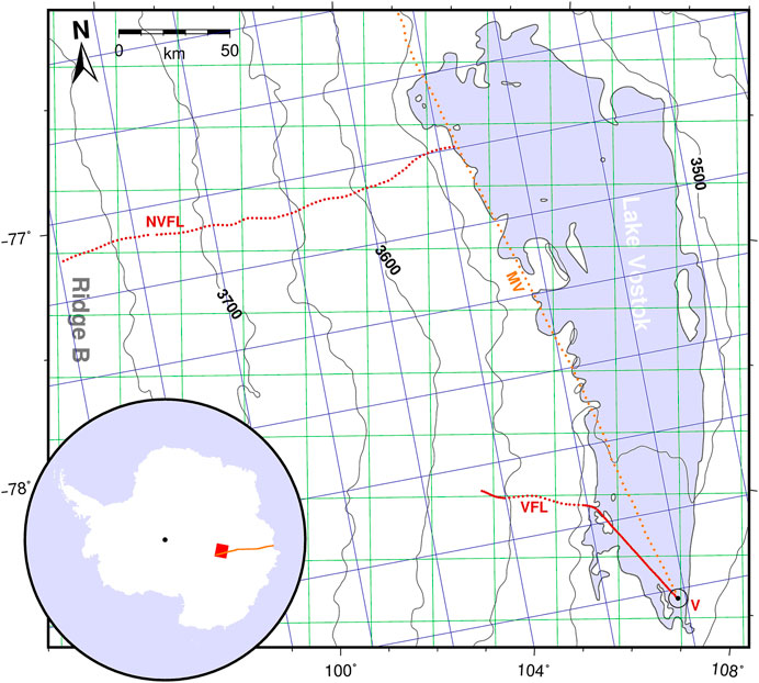
FIGURE 1. Map of the region under investigation. V: Vostok station; tiny red dots: location of accumulation stakes along the VFL and NVFL profiles; orange dots: accumulation stakes along the MV profile. Green and blue gridlines: grid cell boundaries of the regional climate models RACMO and MAR, respectively. Blue shaded area shows subglacial Lake Vostok according to the shoreline from Popov and Chernoglazov (2011). Isohypses depict the ice-surface elevation above WGS84 according to Bamber et al. (2009). The inset shows the location of the map area (red) in Antarctica; orange: MV stake profile between Mirny and Vostok.
The Regional Atmospheric Climate MOdel version 2.3p2 (van Wessem et al., 2018), henceforth referred to as RACMO, is an adaptation of the regional climate model RACMO2 to polar ice sheets, coupled with a snow model, designed to model near-surface climate, the surface energy budget and the SMB over the Greenland and Antarctic ice sheets. Over the AIS it has a horizontal resolution of 27 km. We use the model output for the period from January 1979 through August 2019. It is forced at its lateral boundaries by ERA-Interim reanalysis data (Dee et al., 2011) of pressure, wind, temperature, humidity, sea ice concentration and sea surface temperature every 6 h and with a spatial resolution of 0.75°. The SMB is obtained as the sum of the modeled precipitation, surface sublimation, drifting snow sublimation, drifting snow erosion and meltwater run-off. The interaction of the near-surface air with drifting snow is explicitly modeled. The time-dependent, multilayer, single-column snow model is based on a firn densification model and relates the firn density, temperature and liquid water content to the surface temperature, accumulation and wind speed. The regional climate model MAR version 3.11, henceforth termed MAR, has been developed independently from RACMO (Kittel et al., 2021). It covers the AIS with a horizontal resolution of 35 km and is forced by the ERA5 reanalysis data (Hersbach et al., 2020) over the period January 1979 through December 2019. MAR does not account explicitly for drifting snow processes (erosion, transport, sublimation; Agosta et al., 2019). However, an external blowing snow module (Amory et al., 2020) can be enabled on request. In the following, where not stated otherwise, we use the generic MAR estimates without explicit incorporation of drifting snow processes. An additional model run including the blowing snow module is used to assess the impact of snow drift on the SMB reconstruction. RACMO and MAR are the only two RCMs within the suite analyzed by Mottram et al. (2020) that feature subsurface schemes optimized over snow and ice for Antarctica.
Neither of these models assimilates any SMB observations. Their SMB simulations have been evaluated against the GLACIOCLIM-SAMBA data set (Favier et al., 2013) which includes part of the stake observations along the Mirny-Vostok convoy track (Van Wessem et al., 2014; Agosta et al., 2019; Mottram et al., 2020). The central EAP is evidently underrepresented in the GLACIOCLIM-SAMBA data. Furthermore, those studies (Van Wessem et al., 2014; Agosta et al., 2019; Mottram et al., 2020) extended their comparisons over the entire AIS, but limited themselves to the mean SMB over the entire observation time span available. Here, we analyze also the temporal variations of the SMB time series simulated by the RCMs.
In the Vostok region a reasonably precise SMB reconstruction is a challenge to any continental-scale model. The very low SMB calls for an accurate representation of all involved processes, requiring model parameters tuned to conditions substantially different from, and sometimes even in conflict with, those in the highly dynamic coastal zones more densely sampled by instrumental observations. In this cold environment (mean surface air temperature: -54.9°C, Shibayev et al., 2019) surface melt is absent and the efficiency of the sublimation of both drifting snow and precipitating particles in low-level atmospheric layers is substantially reduced. Drifting snow transport is important and controlled by the surface elevation gradient from Ridge B down to Lake Vostok. The propagation of wind dynamics and precipitation from the peripheral atmospheric forcing so far inland (1,250 km from the nearest coast) is highly sensitive to uncertainties in the model boundary conditions. Yet these extreme conditions prevail not only at Vostok but across the EAP extending over 3 million km2. Therefore, Vostok is representative for the plateau area.
In January 1970 a stake farm was set up about 1.5 km north of Vostok station (VSF; Barkov and Lipenkov, 1978). It consists of 79 stakes spaced every 25 m, forming an equilateral cross of 1 km × 1 km approximately aligned in the cardinal directions (Ekaykin et al., 2020). Between early 1970 and late 2004 (with some interruptions, see Table 1) the height of each stake above the local snow surface was measured once a month. Near every fifth stake the measurement is complemented by the determination of the density of the uppermost 20 cm snow layer. The apparent snow build-up is derived as the difference in stake height between two consecutive measurements. It is averaged over all 79 stakes and multiplied by the mean snow density to yield the snow mass (kg m-2) accumulated during that month. After 2004 these measurements have been continued at a yearly interval (every late December). In this way an SMB time series of annual resolution from 1970 through 2019 (with a gap in 2002–2003) is derived. The temporal coverage of VSF observations is depicted in Figure 2A. In December 1998 a new stake farm was set up (NSF) with identical dimensions and contiguously to the west of the old stake farm. Yearly measurements of this stake farm yield a second annual SMB time series from 1999 through 2019 (with a gap in 2002–2003). The annual SMB time series derived from both stake farms and simulated by the RACMO and MAR models for the grid cells containing the VSF location are shown in Figure 2A. Figure 2B illustrates the monthly SMB time series according to VSF observations and both RCMs during a segment of the common data interval 1979–1994.
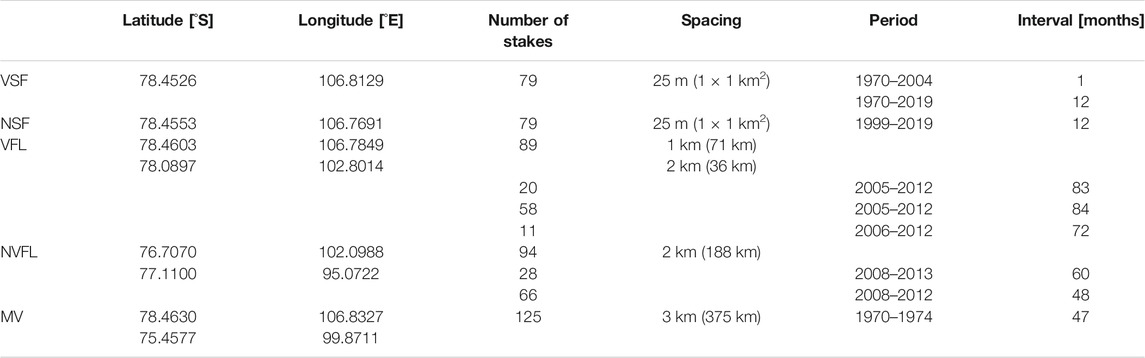
TABLE 1. Summary of the stake observations in the Vostok region used in the comparison. The coordinates indicate the center of the stake farms VSF and NSF, and both termini locations of the profiles VFL, NVFL and MV.
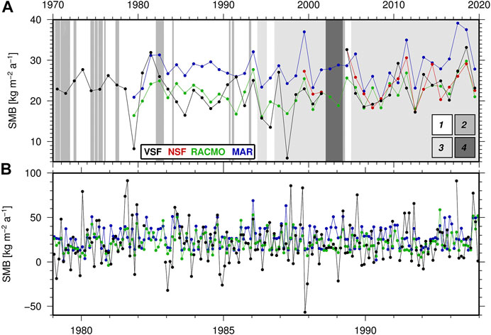
FIGURE 2. Time series of observed and modeled SMB at Vostok. (A) SMB derived from annual observations in the Vostok stake farm (VSF, black) and the new stake farm (NSF, red) and annually cumulated SMB estimated by RACMO (green) and MAR (blue). Background gray shade indicates the stake data coverage: 1 - monthly data; 2 - incomplete monthly data; 3 - annual data; 4 - data void. (B) SMB derived from monthly VSF observations (black) and estimated by RACMO (green) and MAR (blue) during a segment of the common data interval 1979–1994.
In addition to the stake farms close to Vostok station, two stake profiles were set up and measured repeatedly in the region between subglacial Lake Vostok and Ridge B (Ekaykin et al., 2012). The 107 km long VFL profile was set up along the ice flowline through Vostok station upflow toward Ridge B (Figure 1). The profile consists of 89 stakes, spaced every 1 km along the easternmost 60 km and the westernmost 10 km of the profile, and every 2 km between kilometers 60 and 96. While the bulk of stakes was set up and measured for the first time in January 2005, the 11 westernmost stakes were set up in January 2006. The stake measurements were repeated in the 2011/2012 season (Table 1). The snow density of the uppermost 20 cm was determined at every stake. A second, 188 km long profile (NVFL) was set up in January 2008 along a flowline from the NW grounding line of Lake Vostok up to Ridge B (Figure 1). It consists of 94 stakes spaced every 2 km. The measurements at the westernmost 66 stakes (km 58–188) were repeated in January 2012, whereas the easternmost 28 stakes were re-measured in January 2013. The snow density of the uppermost 20 cm was determined at the easternmost ten stakes (20 km), and from there upflow at every fifth stake. Based on these measured densities an empirical relationship between the density and the E-W profile length is derived and applied to interpolate the snow density for the westernmost 84 stakes. The time span between the initial and repeated stake measurements along both profiles varies between 4 and 7 years. Over this time span the SMB is derived for each individual stake from the observed apparent snow build-up, the snow density determined for the stake location and the number of days between both stake measurement dates.
Further stakes were set up in 1970 along the convoy track from Mirny to Vostok at equidistant intervals of 3 km (MV profile). We use measurements of the 125 southernmost stakes of this profile (from Vostok to 375 km north) between January 1970 and December 1973 (Table 1). As these observations are prior to the RCM period they do not allow a direct comparison with model estimates. Nevertheless, they are utilized here to assess the spatial variation scales of the temporal SMB observations.
Ekaykin et al. (2020) have shown that uncorrected stake measurements systematically underestimate the snow build-up and derived SMB due to the progressive densification of the snow layer between the stake base and the surface. An explicit formulation of this effect results in corrections which are, in the Lake Vostok region, too small in magnitude. For this reason we adopt here an empirical generalized densification correction of 8±4% (Ekaykin et al., 2020) which is applied to the SMB estimates derived from all the stake measurements (both stake farms and the three stake profiles).
We consider the SMB as a stochastic process in the two-dimensional space, with the time representing a third dimension. The SMB estimated by the RCMs represent discrete grid cells which suppress any variation on wavelengths shorter than about 50 km. Individual stake observations, in turn, reflect variations on a wide range of spatial scales as short as sub-meter (e.g., sastrugi). SMB observations averaged over the VSF reduce the small-scale variations with wavelengths shorter than 1 km. In our case, stake observations and RCMs describe the temporal SMB variation through time series with a maximum resolution of one month. This implies, first, a low-pass filtering (filter width of one month) and, second, a sampling at discrete points in time (once a month) of the continuous stochastic process. A large part of the observational data consists of mean SMB estimates over time intervals of one year (VSF, NSF) or several years (MV, VFL and NVFL profiles). An assessment of the accuracy of the stake observations is crucial for the interpretation of their comparison with the RCM simulations. Differences between stake farm averages and RCM estimates (modeled SMB minus observed SMB, henceforth M-O differences) result from the combined effect of the following contributions: (A) the deviation of the stake observations from the true value over the 1 × 1 km2 area (i.e., local variability), (B) the difference between the true value over 1 × 1 km2 and the true value over the model grid cell (i.e., short-wavelength processes which average out over 27 × 27 or 35 × 35 km2), and (C) the deviation of the model value from the true value over the model grid cell (i.e., model errors). Contribution A to the SMB derived from stake observations is dominated by small-scale variations in snow build-up. Observational uncertainties are expected to have a minor effect. For this reason, in the following we refer to “local variability” when addressing the accuracy, or uncertainty, of observed SMB.
Confidence intervals for the annual stake farm observations, that is, contribution A, are derived from the standard deviation of the differences between the simultaneous observations in VSF and NSF, assuming that both stake farms yield equally accurate SMB averages and that the differences do not contain a significant differential SMB signal.
The information contained in the monthly and annual SMB observations in VSF is combined in one time series. Gaps in the monthly record are filled by distributing the remainder of the annual SMB after subtraction of all sampled monthly values uniformly over the missing months. For all years without monthly readings the monthly values are set constant throughout the year and proportional to the annual mean rate. During the gap in the annual record (2002–2003) the mean SMB throughout the entire annual VSF data set is adopted. This combined time series provides an 11-years long record of continuous monthly observations 1983–1994 with only four short gaps (of one or two months duration) complemented based on the annual record (Figure 2B). This continuous high-resolution time series is used to analyze the statistical properties of the VSF observations. In particular, the autocorrelation and autocovariance functions of monthly VSF observations are determined (Figure 4). A linear model (mean value and rate) was subtracted from the time series prior to the autocovariance computation in order to assure a zero expectation and stationarity.
The VSF time series are used to explore the ability of the RCMs to reproduce the observed temporal variation of the SMB over different time scales (Section 3.2). The modeled SMB are evaluated as the RACMO or MAR values in their grid cell that contains the VSF location, without further spatial interpolation. In a separate analysis (Section 3.3) we test an inverse-distance weighted interpolation between the four grid cells closest to VSF, employing linear, quadratic and cubic interpolation schemes, in order to explore the eccentric location of VSF relative to the model grid cells as an explanation for systematic M-O differences. For each month contained in the monthly VSF record (no interpolated values included), the M-O differences are calculated. The comparison includes a scatter plot (Figure 5A), the least-squares estimation of linear regression parameters (slope s), the mean value (Δ) of the M-O differences, the root-mean-square deviation (rms), and the Pearson correlation coefficient (r). The monthly SMB simulated by the RCMs for the Vostok grid cell are cumulated to annual mean SMBs. Annual M-O differences are derived from these annual model time series and the annual VSF observation record (no interpolated values included). The annual SMB time series are compared in a similar way as the monthly values (scatter plot, linear regression, statistical parameters; Figure 5B). The mean M-O differences, their standard deviations and histograms are used to quantify possible biases between RCM estimates and stake farm observations and to determine their statistical significance according to a t-test (Figures 5C,D). The consistency between stake measurements and RCMs regarding the mean SMB over several years is explored based on the combined time series of monthly and annual data. The temporal variation of the mean SMB is derived by averaging this combined record over a moving window of a given integration interval. Likewise, for the RCM results, time series of mean SMB are derived by averaging the monthly simulations within a moving window corresponding to the chosen integration interval (Figure 6).
The mean annual cycle is derived by stacking monthly SMB anomalies observed in VSF (Figure 7). For this purpose, the mean SMB throughout the year in question is subtracted from each SMB value. This reduces the distortion of the mean annual signal by interannual SMB variations. We restrict the stacking of the observations to those 11 years between 1979 and 1995, for which a complete monthly observation record (i.e., without data gap) and RCM estimates are available. Relaxing this restriction would allow to increase the number of realisations in each month from 11 to 20, but has no significant impact neither on the mean annual cycle nor on its formal uncertainty. The mean annual cycle of the modeled SMB is determined in the same way, restricting the stacking of the residual SMB (i.e., after subtraction of the mean SMB of that year) only to those years included in the observation stacking. The confidence interval of the mean annual cycle is derived from the formal uncertainty of the mean value of each month as
The SMB observations along the MV and VFL profiles are used to assess the combined effect of contributions A+B (Section 3.1). First, the accuracy of a single profile stake observation and its spatial correlation are determined. For this purpose, the very long-wave SMB variation is subtracted from the SMB observed along the profiles, applying polynomials of degree 2 (MV) or 1 (VFL; Figure 3). The standard deviation of the individual stake observations along the profile, after removing the very long-wave model, yields an accuracy estimate of the multi-year SMB observed at a single profile stake. This uncertainty is interpreted as the combined effect of contributions A+B. Its comparison with the single-stake variability in VSF, as propagated from the uncertainty estimated for the farm averages, allows to isolate the contribution B to multi-year mean SMB.
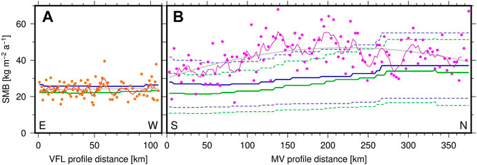
FIGURE 3. Spatial variability of multi-year SMB observed along stake profiles in the Vostok region. (A) VFL profile: mean SMB over 7 years observed at individual stakes (orange dots); spatially low-pass filtered SMB variation by averaging over five contiguous stakes (red curve); linear model used to remove the very long-wave SMB variation in the autocovariance calculation (gray line); SMB averaged over the observation period according to RACMO (green) and MAR (blue); mean SMB observed over the same period in VSF: 21.9 kg m-2 a-1. (B) MV profile: mean SMB over 4 years observed at individual stakes 1970–1974 (purple dots); spatially low-pass filtered SMB variation by averaging over five contiguous stakes (purple curve); quadratic model (gray curve); mean SMB averaged over the entire model period 1979–2019 (solid) with its temporal standard deviation (dashed) according to RACMO (green) and MAR (blue); mean SMB observed over the same period in VSF: 24.3 kg m-2 a-1.
The ability of the RCMs to reproduce the spatial SMB variation in the Lake Vostok-Ridge B region is assessed based on the SMB derived from the stake measurements along the VFL and NVFL profiles (Section 3.3). The monthly model time series of the grid cells corresponding to each stake location, without spatial interpolation, are cumulated between the dates of the stake measurements (accounting for incomplete months proportionally to the number of days) and divided by the number of days between both measurements. The observational results are averaged within the bounds of the individual grid cells in order to reduce the noise inherent to individual stake observations (cf. Agosta et al., 2019). Since the observation periods are practically identical for all the stakes within one model grid cell, no weighting was applied among the individual stakes. Due to the different grid geometry, this analysis has to be performed separately for both RCMs (Figure 9).
The standard deviation of the differences between the simultaneous observations in the contiguous VSF and NSF amounts to 3.4 kg m-2 a-1. We infer an uncertainty of ±2.4 kg m-2 a-1 for an annual SMB averaged over one stake farm (contribution A to the M-O differences). The standard deviation of the monthly SMB observations in VSF suggests an accuracy of ±25.5 kg m-2 a-1. The autocorrelation function of the monthly SMB anomalies in the continuous 11-years VSF record (Figure 4A) is characterized by a low correlation, essentially within ±0.2, for all τ>0. This indicates that the variation in monthly SMB values is largely uncorrelated in time and dominated by a random component (white noise). The smoothed autocorrelation function, obtained by a running average over five contiguous τ values, reveals a small persistent annual period in the SMB variation with local correlation maxima at multiples of 12 months. The autocorrelation function of the 50-years record of annual VSF observations (Figure 4B) confirms the very low temporal correlation over longer time spans which would also indicate a white noise behavior of the observed SMB variations with respect to the mean value.
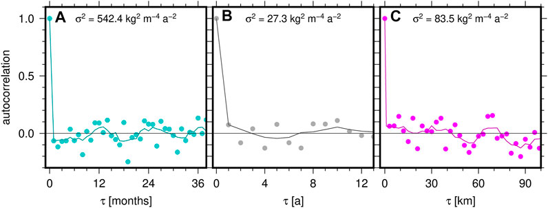
FIGURE 4. Autocorrelation functions of the SMB derived from stake observations. Continuous curves show the autocorrelation for τ > 0, low-pass filtered by averaging over five τ-values. The indicated variance
The SMB observed along the 375 km long MV stake profile (Figure 3B) allows us to analyze the spatial scale dependence of SMB variations over the wavelengths resolved by the RCM. Figure 4C shows the autocorrelation function of this SMB profile (after subtracting a trend polynomial of degree 2, Figure 3). It reveals a very low correlation for all τ>0, generally within ±0.2. This demonstrates that random variations (white noise), for example related with drifting snow processes, dominate the local SMB anomalies observed at individual stakes spaced at 3 km intervals. The variance along the profile is 84 kg-2 m-4 a-2. This suggests that the local variability of the multi-year SMB at a single stake is 9.1 kg m-2 a-1. For comparison, the uncertainty of the SMB observed in VSF over 47 months amounts to ±0.6 kg m-2 a-1 for the stake farm average. This relates to a local variability of 5.4 kg m-2 a-1 at a single stake when the individual stakes in the farm are assumed to be uncorrelated. The VFL profile yields (after subtraction of a linear model) a local variability of 4.4 kg m-2 a-1 for a single-stake multi-year observation in this profile over a mean interval of 83 months. A stake farm average over this interval is accurate to ±0.3 kg m-2 a-1, suggesting a single-stake variability of 3.1 kg m-2 a-1 when neglecting any correlation between the farm stakes.
The differences in the single-stake variability between VSF and both profiles amount to 3.7 kg m-2 a-1 (MV) and 1.3 kg m-2 a-1 (VFL). They represent conservative estimates of contribution B to M-O differences over 47 and 83 months, respectively. First, these estimates of contribution B do not discriminate between spatial wavelengths. They include the variation on spatial scales between the model grid cell dimension and that of the subtracted very long-wave models. Second, the VSF single-stake variability introduced in this comparison is too optimistic because spatial correlation between the individual stakes of the farm is certainly effective but not accounted for in the estimation. Third, these B estimates probably include also part of the observational uncertainty along the profiles, as the stake observations in the farms are expected to be of superior accuracy than those along MV and, perhaps to a lesser extent, VFL. We may, therefore, regard the differences in single-stake variability as upper bounds for contribution B to M-O differences over 47 and 83 months. On the other hand, the effect of contribution B is expected to decrease with increasing time scales, as the comparison of our B estimates for two different observation periods confirms. However, the available data do not allow to rigorously disentangle the spatial and temporal scale dependencies of contribution B. Adopting the B estimate derived from the single-stake variability along MV as representative also for farm averages over one year, the combined effect of contributions A+B on annual M-O differences between RCM estimates and VSF amounts to
The time series of both monthly readings (Figure 2B) and annual SMB values (Figure 2A) reveal, first, a much broader variation of the VSF observations compared to the estimates of both RCMs and, second, a positive offset of the SMB simulated by MAR compared to RACMO and the stake observations. Both findings are also evident in the scatter plots in Figure 5A (monthly SMB readings) and Figure 5B (annual mean SMB). The M-O differences between the monthly VSF observations (1979–2004; 187 values) and the RACMO model estimates have a mean value of +0.7 kg m-2 a-1 and a standard deviation of 22.4 kg m-2 a-1. For MAR the mean value of the monthly M-O differences amounts to +6.3 kg m-2 a-1 and the standard deviation to 24.1 kg m-2 a-1. The variance of the SMB reconstructed by RACMO and MAR amounts to 18 and 25%, respectively, of the variance of the monthly observations. Both the linear regression (slope s) and the rather moderate, yet statistically significant (99% confidence), correlation demonstrate that either of the models contain a common signal with the observations. RACMO fits the observed variation better than MAR, regardless of the offset. For RACMO, the regression slopes are 0.96 and 1.04 at monthly and annual resolution, respectively, while for MAR these slopes amount to 0.55 and 0.69. However, the M-O differences amount to 84% (RACMO) and 98% (MAR) of the observed monthly variance, reflected in Figure 5A by the large scatter of the observations about the regression lines and the rms deviations in excess of the observed mean value.
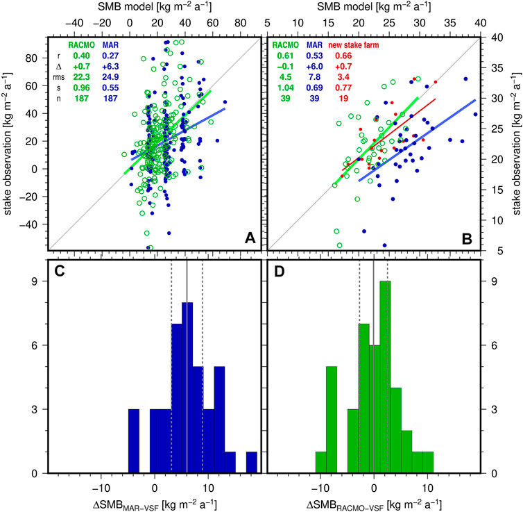
FIGURE 5. Comparison of SMB estimated by RACMO (green) and MAR (blue) with observations in stake farms at Vostok station over different time scales. (A) Scatter plot of monthly SMB. Statistics: Pearson correlation coefficient (r), mean difference model minus observation (Δ), root-mean-square deviation (rms), slope (s) of a linear regression, number of data pairs (n). (B) Scatter plot of annual SMB. (C) Histogram of annual M-O differences between MAR and VSF (n = 39). Gray line indicates the mean value (i.e., Δ; solid) and its 99.9% confidence interval (according to a t-test; dashed). The confidence interval of the mean M-O difference is clearly different from zero, indicating a statistically significant bias. (D) Histogram of annual M-O differences between RACMO and VSF (n = 39).
The comparison of annual SMB observations with the annually cumulated model estimates (Figure 5B) indicates an increase in correlation and a decrease in rms deviation relative to the monthly comparison. Over the period of simultaneous annual SMB values of VSF and the RCMs (1979–2019; 39 annual values) the M-O differences have mean values of -0.1 kg m-2 a-1 (RACMO) and +6.0 kg m-2 a-1 (MAR), and standard deviations of 4.5 kg m-2 a-1 (RACMO) and 5.0 kg m-2 a-1 (MAR). The standard deviations of the annual M-O differences confirm our estimate of 4.4 kg m-2 a-1 as a conservative quantification of the combined effect of contributions A+B. Histograms of the annual M-O differences are shown in Figure 5C (MAR) and Figure 5D (RACMO). MAR’s M-O differences are statistically significant at a 99.9% confidence level, indicating that the annual SMB observed in VSF and modeled by MAR do not belong to the same population. This bias corresponds to 30% of the mean monthly observed SMB of 21 kg m-2 a-1 (contribution C). The RACMO M-O differences are statistically not significant, also at lower confidence levels. The annual comparison (Figure 5B) reveals furthermore a lower variability in the modeled SMB which amounts to 34% (RACMO) and 57% (MAR) of the variance of the annual observations; a superior fit of RACMO compared to MAR according to the regression slope and correlation coefficient; and M-O differences which correspond to 63% (RACMO) and 78% (MAR) of the observed variance. Figure 5B includes also the comparison of the annual SMB observations in VSF and NSF over the 19 years period of simultaneous data (1999–2019).
Figure 6A shows the variation of the mean SMB derived from VSF observations and RCM over the observation period for two different integration intervals. The comparison of mean rates integrated over two and five years indicates, for observations and RCM similarly, a variance reduction of 60–65%. The multi-year SMB simulated by RACMO represent, independent of the integration interval, 45% of the variance of the SMB derived from the stake observations. The 5-years SMB of VSF and RACMO reveal a common long-term signal characterized by a reversal of the trend at a minimum around 1996. The largest deviation between RACMO and VSF 5-years mean SMB occurs in the 1980s and might be caused by an inferior accuracy of the global forcing by ERA-Interim in those early times. MAR’s biased SMB estimates cause, as expected, also a bias in the multi-year SMB with a mean M-O difference over the common data period of +8 kg m-2 a-1. The M-O difference of 5-years SMB varies with time, with a maximum effect in the late 1990s and an increase during the last decade. The cumulated SMB at Vostok over the model period (1979–2019) is shown in Figure 6B. It highlights an excellent agreement between the stake observations and RACMO. The long-term mean SMB (1816–2004) derived by Ekaykin et al. (2004) from stacked snow pits and shallow cores is included for comparison.
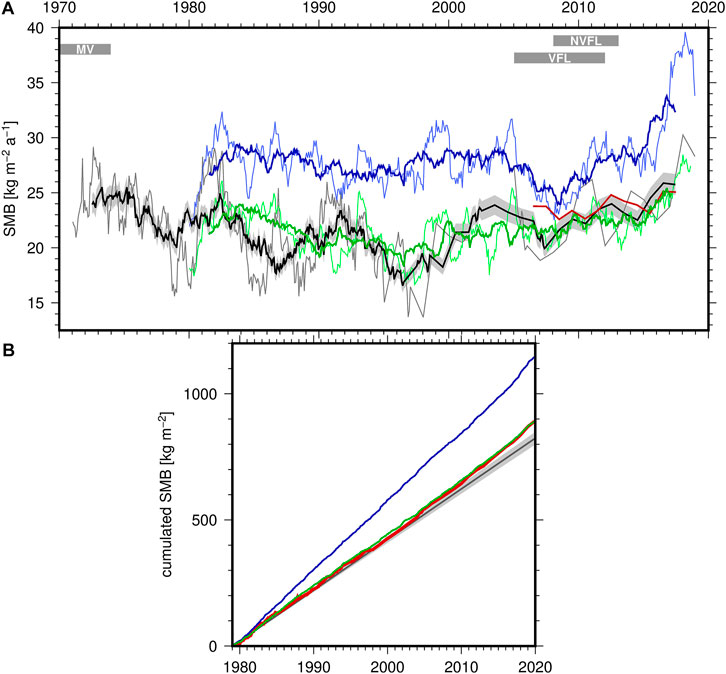
FIGURE 6. Comparison of long-term mean SMB derived from stake observations at Vostok with RCM simulations. (A) Variation of multi-year mean SMB over the observation period as derived from observations in the Vostok stake farm (black) and new stake farm (red) and from RACMO (green) and MAR (blue) model estimates. Thin curves: SMB averaged over 2 years; thick curves: SMB averaged over 5 years; light gray band about VSF 5-years mean SMB: uncertainty of the generalized densification correction applied. Horizontal gray bands indicate the periods covered by the stake observations in the MV, VFL and NVFL profiles. (B) SMB cumulated over the model period 1979–2019; the gray line depicts the mean accumulation rate over the period 1816–2004, and its uncertainty, as derived by Ekaykin et al. (2004) from stacked snow pits and shallow cores at Vostok.
A temporal partitioning of the variance in the VSF monthly SMB time series indicates that 5% (31.4 kg2 m-4 a-2) of the observed variance is due to interannual variation and 14% (85.3 kg2 m-4 a-2) due to the mean annual cycle. The model time series show a comparable relative contribution from interannual variability (RACMO: 7%, 7.7 kg2 m-4 a-2; MAR: 5%, 7.4 kg2 m-4 a-2), but a much smaller seasonal contribution (RACMO: 2%, 2.2 kg2 m-4 a-2; MAR: 2%, 3.5 kg2 m-4 a-2). Thus, the seasonal SMB cycle deserves particular attention.
The mean annual cycle of the VSF SMB observations in Figure 7 reveals a seasonal variation with a minimum during polar day. This variation is statistically significant and consistent with the mean annual cycles of observed meteorological parameters. Nevertheless, neither of the RCMs reproduces an appreciable seasonal SMB variation at Vostok. While a least-squares fit to the observed monthly SMB anomalies yields annual and semi-annual amplitudes of 10 and 8 kg m-2 a-1, respectively, these amplitudes amount to only 2 and 1 kg m-2 a-1 for either of the models. Climatic forcing of the annual SMB cycle is expected to vary only insignificantly within the model grid cells. Small-scale effects contained in the VSF observations cannot explain the occurrence of this persistent periodic signal. Figure 7 suggests that the observed seasonal SMB variation at Vostok is to a large extent due to the seasonal precipitation distribution. The precipitation cycle is similar in magnitude (annual and semi-annual amplitudes of 11 and 4 kg m-2 a-1) and roughly in phase with that of the observed SMB. Small differences in the shape of both annual cycles might be caused by the different amount and time span of SMB and precipitation data, but reflect also the modulation by other, simultaneous processes. Surface sublimation is controlled by the air temperature and small in the Vostok environment. Nevertheless, the steep temperature increase at the transition from polar night to polar day contributes, through a transitory activation of the sublimation (Ekaykin et al., 2004), to the pronounced decrease in SMB toward the end of the year. Drifting snow erosion and deposition might also influence the seasonal SMB variation. The mean annual cycles of both air temperature and wind speed are reasonably well reproduced by both RCM, despite a slight underestimation of the wind speed amplitude. However, the stacked mean annual signals of the monthly precipitation sums estimated by RACMO and MAR are inconsistent with the observed seasonal cycle. In fact, these mean model signals represent no harmonic seasonal behavior, with annual and semi-annual amplitudes that are one order of magnitude smaller than those of the observed variation and thus nonsignificant. This explains the lack of seasonal variation in the modeled SMB at Vostok very likely as a consequence of the missing precipitation cycle of the RCMs. As a consequence also the seasonal variation in near-surface snow density simulated by both RCMs is suppressed.
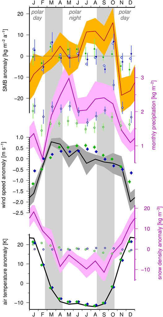
FIGURE 7. Mean annual cycle of SMB and selected meteorological parameters at Vostok station. Top: Monthly SMB anomalies according to Vostok stake farm observations (red) and their formal uncertainties (orange) stacked over 11 years of complete monthly records between 1979 and 1995, compared to analogously stacked monthly SMB anomalies according to RACMO (green) and MAR (blue). Blue open diamonds indicate the identically stacked SMB estimates by MAR including the blowing snow module (Amory et al., 2020). Below (top to bottom) stacked mean annual cycles of monthly: precipitation sums (1979–2017; AARI, 2020), anomalies of wind speed (1979–2006; Reader Project, 2015), anomalies of near-surface snow density (VSF observations, same 11 years as SMB), and near-surface air temperature anomalies (1979–2016; AARI, 2020) at Vostok station are shown. RACMO (green) and MAR (blue) estimates of these parameters are stacked over periods identical to the observation stack. Gray bands in the background mark the transitions between polar day and polar night.
In an attempt to shed light on the cause of the bias in SMB estimates by MAR over different time scales, we examine the precipitation record at Vostok station (AARI, 2020). For 25 years between 1979 and 2014 there are complete annual precipitation sums, annual SMB observations in VSF and RCM estimates of precipitation and SMB available. Over these years, the mean SMB and precipitation observed at Vostok amount to 21.3 and 19.0 kg m-2 a-1, respectively. RACMO reproduces these values almost perfectly with a mean SMB of 21.4 kg m-2 a-1 and a mean precipitation of 19.7 kg m-2 a-1. MAR yields a mean SMB of 27.0 kg m-2 a-1, thus overestimating the observed SMB by 27%. The precipitation estimated by MAR at 24.3 kg m-2 a-1 exceeds the observed precipitation in a very similar proportion of 28%. This leads us to suggest that the model precipitation is the principal source of MAR’s SMB bias. The latter is not explainable by drifting snow processes not being incorporated in this model. A model run incorporating the external blowing snow module (Amory et al., 2020) yields SMB values on average 2.6 kg m-2 a-1 larger than the generic MAR estimates. This suggests that deposition dominates over erosion at Vostok, and the modeled snow drift contribution is very close to the observed excess of SMB over precipitation (21.3 - 19.0 = 2.3 kg m-2 a-1). The SMB surplus due to drifting snow distributes fairly uniformly over the year (Figure 7, top, blue diamonds compared to blue dots). However, this contribution further increases the M-O differences from +6.3 to +8.9 kg m-2 a-1. Also the wind speed and direction observed at Vostok station over 22 years (1979–2006; Reader Project, 2015) are better reproduced by RACMO than by MAR. Both RCMs underestimate the daily wind speeds, RACMO by 42% and MAR by 50%. The mean wind direction, as derived from time-averaged wind velocity components, agree between RACMO and the observations within 20°, whereas MAR’s mean wind direction differs by 30° from the observed one. This might suggest the representation of the local atmospheric circulation to be a possible cause for the overestimation of the precipitation.
Figure 3 reveals a substantial variation in multi-year mean SMB over short distances (i.e., individual stakes). In Figure 8 we compare the multi-year SMB observed along the VFL, NVFL and MV profiles with the wind-parallel surface curvature in order to assess the impact of the local surface topography on the SMB through conditioning the wind-driven snow erosion and deposition. For this purpose we use a recent digital elevation model (DEM, Howat et al., 2019), sampled to 100 m horizontal resolution. The DEM gradient in the mean wind direction (according to RACMO estimates of local wind vector components averaged over the model period 1979–2019) represents the wind-parallel surface slope. The gradients of this wind-parallel slope, evaluated at the stake locations and in the mean wind direction, yield the wind-parallel surface curvature shown in Figure 8. Along the VFL profile (Figure 8B, 7-years observation period) the two major positive local SMB anomalies coincide with concave surface curvature (troughs), as already noted by Ekaykin et al. (2012). However, negative SMB anomalies do not seem to generally coincide with convex surface curvature, and along NVFL and MV a correlation between curvature and SMB is not as evident. This might suggest that a 4-years observation period (NVFL, MV) is too short to let the topography effect stand out against random variations (Figure 4C). Other processes have to be considered in addition to explain this short-wavelength SMB variability, as evidenced e.g., by the S-N increase along the southernmost 150 km of the MV profile. A similar analysis of the wind-parallel slope and the absolute maximum curvature and slope (i.e., independent of the wind direction) does not provide further insights into the topographic control of SMB variations. It has to be noted, though, that not only stake observations but also DEMs are subject to noise which is enhanced by the twofold differentiation in the curvature determination.
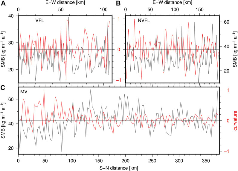
FIGURE 8. Comparison of the spatial variation in observed multi-year SMB (gray) and wind-parallel surface curvature (red). The surface curvature is derived from the REMA DEM (Howat et al., 2019) at 100 m resolution in the direction of the mean wind direction according to RACMO (1979–2019) and normalized along each profile. Positive curvature indicates a concave surface (trough). (A) VFL profile (observation interval 7 years). (B) NVFL profile (4 years). (C) MV profile (4 years).
Figure 9 presents the comparison of multi-year SMB derived from the stake observations along the VFL and NVFL profiles with the cumulated SMB model estimates. The observed SMB is averaged over all the stakes within the model grid cell boundaries of the corresponding RCM estimates. This comparison reveals an overall satisfactory agreement between stake observations and the RACMO model. The SMB increase from the southern (VFL) to the northern (NVFL) profile is consistently reproduced by both observation and model, although RACMO slightly underestimates the SMB derived from stake measurements along VFL by applying the generalized 8% snow densification correction. The comparison shows also that the systematic bias in SMB estimated by MAR is not a local effect restricted to Vostok station (Figure 5) but likely affects a broader region between Ridge B and Lake Vostok.
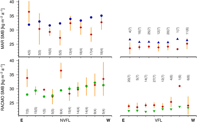
FIGURE 9. Comparison of SMB estimated by RACMO (green) and MAR (blue) with multi-year SMB observed along the VFL and NVFL stake profiles. Stake-derived SMB averaged within the MAR (top, blue) and RACMO (bottom, green) model grid cells (red); orange: uncertainty of the cell averages. For each model grid cell the number of stakes (and years between repeated observations, i.e., integration interval) are indicated.
The mean difference between SMB estimates by MAR and stake observations along the VFL and NVFL profiles amounts to +2.3 kg m-2 a-1. This discrepancy is substantially smaller in magnitude than the average 5-years SMB bias at Vostok station (+8 kg m-2 a-1). In part, this is an effect of the profile observation period coincident with the minimum deviation between MAR and observed multi-year SMB at Vostok (Figure 6). We conclude that a positive bias affects the SMB reconstructed by MAR over a larger region between Ridge B and Lake Vostok, even though the mean bias over that region is probably smaller than the bias derived at Vostok station. It could be speculated that the MAR model biases revealed at Vostok over different time scales could be caused by the eccentric location of VSF relative to the model grid cell (Figure 1). VSF’s location close to a continental divide of atmospheric circulation might imply significant gradients, e.g., in humidity transport, over distances comparable to the grid cell dimensions which could produce a systematic bias between the precipitation, and thus SMB, MAR estimates in the cell center and that observed at Vostok. In this case, an interpolation across the divide should reduce this bias significantly. To test this hypothesis, we interpolate the monthly MAR estimates to the VSF location as an inverse-distance weighted average of the SMB simulated for the four nearest grid cells. However, this interpolation does not reduce the mean M-O difference (from +6.3 to +6.4 kg m-2 a-1). The interpolation has a similarly insignificant impact on the annual M-O differences. RACMO, with its grid cell center located only slightly closer to VSF than MAR, does also not improve its fit to the VSF record by the interpolation. These comparisons are insensitive to the applied interpolation scheme (linear, quadratic, or cubic). The detection of MAR’s SMB bias all over the studied region, the relatively small contribution of drifting snow to SMB (roughly 10%), and the superior performance of RACMO despite facing the same challenges posed by the short-wavelength processes make it likely that the cause of MAR’s bias is to be sought in the atmospheric circulation and humidity transport over spatial scales exceeding a few model grid cells around Vostok.
Our comparison reveals a clear common signal in the SMB time series derived from stake observations and continental-scale atmospheric models. This proves success in both observing and modeling SMB variations under conditions as peculiar as those encountered at Vostok.
Our results show, first, an impressive agreement between RACMO and densification-corrected stake observations in annual and long-term mean SMB at Vostok station. The regression slope between modeled and observed temporal variations at both monthly and annual resolution is close to 1.0. No statistically significant difference is established between the observed and modeled temporal variations in annual mean SMB. As the insignificance of the differences depends on the noise level of the observations, the quantification of confidence intervals of the observed SMB is an essential element of the study.
Second, a systematic positive bias is detected in MAR’s SMB estimates, which varies between +2 and +6 kg m-2 a-1 over the time and space sampled by our observations. This bias is very small compared to SMB observed at the ice sheet margins. If the bias established at Vostok were valid for the entire EAP, it would imply an overestimation of the AIS mass balance of 18 Gt a-1, i.e., on the order of 20% of recent estimates. However, the limited spatial extent of our data does not allow robust conclusions about the integral performance of either RCM over the AIS (e.g., Mottram et al., 2020).
Third, our comparison indicates a poor representation of the annual SMB cycle at Vostok by either RCM. This is largely attributable to a seasonal precipitation distribution inconsistent with the meteorological record at Vostok. The difference in the spatial scales sampled by our observations and the RCMs does not affect this finding substantially.
Finally, our analysis demonstrates the potential of the Vostok stake data set to tune RCM parameters toward an improved representation of the SMB over the EAP. Its unique location qualifies Vostok as a benchmark validation site. On the one hand, the extremely flat ice surface atop the subglacial lake minimizes slope-dependent effects on SMB observations (e.g., transient dunes and mega-dunes). On the other hand, its location at the boundary between humidity sources in the Pacific and Indian sectors makes Vostok highly sensitive to the large-scale atmospheric circulation simulated by RCMs.
The stake observation data used in this study are accessible at the website of the Arctic and Antarctic Research Institute-Climate and Environment Changes Research Laboratory http://cerl-aari.ru/index.php/smb-vostok/. Monthly summaries of meteorological parameters observed at Vostok station can be found in the website of the Arctic and Antarctic Research Institute http://www.aari.aq/data/data.php?lang=1&station=6#temp. Synoptic observations from Vostok station can be found in the website of the READER project https://legacy.bas.ac.uk/met/READER/surface/stationpt.html.
AR led the study and wrote the original draft. AE and VL provided the stake observation data. MW and AG carried out analysis and software development. MH and RD contributed to the conceptualization and methodology. SP performed analysis and validation; MS administrated the project. All authors provided comments and edits on the manuscript.
This work was jointly funded by the German Research Foundation (DFG, grant SCHE 1426/20-1) and the Russian Foundation for Basic Research (RFBR, grant no. 17-55-12003 NNIO). The work of MW was funded by DFG through grant HO 4232/4-1 “Reconciling ocean mass change and GIA from satellite gravity and altimetry (OMCG)” in the Special Priority Program (SPP) 1889 “Regional Sea Level Change and Society.” The glaciological fieldwork was supported by the Russian Foundation for Basic Research (grants 10-05-93106 and 17-05-01168) and by the Russian Geographical Society.
The authors declare that the research was conducted in the absence of any commercial or financial relationships that could be construed as a potential conflict of interest.
This work builds on the efforts, deprivations and field-glaciological skill of many generations of wintering teams at Vostok. The logistic support from the Russian Antarctic Expedition is highly appreciated. The SMB and meteorological parameters estimated by the regional climate models were provided to the authors by Jan Melchior van Wessem (RACMO) and Cécile Agosta, Christoph Kittel, and Charles Amory (MAR). All figures are produced using the Generic Mapping Tools (Wessel et al., 2019).
Agosta, C., Amory, C., Kittel, C., Orsi, A., Favier, V., Gallée, H., et al. (2019). Estimation of the Antarctic Surface Mass Balance Using the Regional Climate Model MAR (1979–2015) and Identification of Dominant Processes. The Cryosphere 13, 281–296. doi:10.5194/tc-13-281-2019
Amory, C., Kittel, C., Le Toumelin, L., Agosta, C., Delhasse, A., Favier, V., et al. (2020). Performance of MAR (v3.11) in Simulating the Drifting-Snow Climate and Surface Mass Balance of Adelie Land, East Antarctica. Geoscientific Model. Development Discuss. 2020, 1–35. doi:10.5194/gmd-2020-368
Bamber, J. L., Gomez-Dans, J. L., and Griggs, J. A. (2009). A New 1 Km Digital Elevation Model of the Antarctic Derived from Combined Satellite Radar and Laser Data – Part 1: Data and Methods. The Cryosphere 3, 101–111. doi:10.5194/tc-3-101-2009
Barkov, N. I., and Lipenkov, V. Y. (1978). Snow Accumulation in the Area of Vostok Station in 1971–1973. Informatsionnyi Bulleten’ SAE 98.
Dee, D. P., Uppala, S. M., Simmons, A. J., Berrisford, P., Poli, P., S, K., et al. (2011). The ERA-Interim Reanalysis: Configuration and Performance of the Data Assimilation System. Q. J. Roy. Meteorol. Soc. 137, 553–597. doi:10.1002/qj.828
Ekaykin, A. A., Kozachek, V. A., Lipenkov, V. Y., and Shibaev, Y. A. (2014). Multiple Climate Shifts in the Southern Hemisphere over the Past Three Centuries Based on Central Antarctic Snow Pits and Core Studies. Ann. Glaciology 55, 259–266. doi:10.3189/201AoG66A189
Ekaykin, A. A., Lipenkov, V. Y., Kuzmina, I. N., Petit, J. R., Masson-Delmotte, V., and Johnsen, S. J. (2004). The Changes in Isotope Composition and Accumulation of Snow at Vostok Station, East Antarctica, over the Past 200 Years. Ann. Glaciology 39, 569–575. doi:10.3189/172756404781814348
Ekaykin, A. A., Lipenkov, V. Y., and Shibaev, Y. A. (2012). Spatial Distribution of the Snow Accumulation Rate along the Ice Flow Lines between Ridge B and Lake Vostok. Ice & Snow 4, 122–128.
Ekaykin, A. A., O, V. D., Lipenkov, V. Y., and Masson-Delmotte, V. (2017). Climatic Variability in Princess Elizabeth Land (East Antarctica). Clim. Past 13, 61–71. doi:10.5194/cp-13-61-2017
Ekaykin, A. A., Teben’kova, N. A., Lipenkov, V. Y., Tchikhatchev, K. B., Veres, A. N., and Richter, A. (2020). Underestimation of Snow Accumulation Rate in Central Antarctica (Vostok Station) Derived from Stake Measurements. Russ. Meteorology Hydrol. 45, 132–140. doi:10.3103/s1068373920020090
Favier, C., Agosta, C., Parouty, S., Durand, G., Delaygue, G. D., Gallée, H., et al. (2013). An Updated and Quality Controlled Surface Mass Balance Dataset for Antarctica. The Cryosphere 7, 583–597. doi:10.5194/tc-7-583-2013
Groh, A., Horwath, M., Horvath, A., Meister, R., Sørensen, L. S., Barletta, V. R., et al. (2020). Evaluating GRACE Mass Change Time Series for the Antarctic and Greenland Ice Sheet–Methods and Results. Geosciences 9, 415. doi:10.3390/geosciences9100415
Hersbach, H., Bell, B., Berrisford, P., Hirahara, S., Horányi, A., Muñoz-Sabater, J., et al. (2020). The ERA5 Global Reanalysis. Q. J. R. Meteorol. Soc. 146, 1999–2049. doi:10.1002/qj.3803
Howat, I. M., Porter, C., Smith, B. E., Noh, M.-J., and Morin, P. (2019). The Reference Elevation Model of Antarctica. The Cryosphere 13, 665–674. doi:10.5194/tc-13-665-2019
Kittel, C., Amory, C., Agosta, C., Jourdain, N. C., Hofer, S., Delhasse, A., et al. (2021). Diverging Future Surface Mass Balance between the Antarctic Ice Shelves and Grounded Ice Sheet. The Cryosphere 15, 1215–1236. doi:10.5194/tc-15-1215-2021
Lenaerts, J. T. M., Medley, B., van den Broeke, M. R., and Wouters, B. (2019). Observing and Modeling Ice Sheet Surface Mass Balance. Rev. Geophys. 57, 376–420. doi:10.1029/2018RG000622
Lenaerts, J. T. M., Vizcaino, M., Fyke, J., van Kampenhout, L., and van den Broeke, M. R. (2016). Present-day and Future Antarctic Ice Sheet Climate and Surface Mass Balance in the Community Earth System Model. Clim. Dyn. 47, 1367–1381. doi:10.1007/s00382-015-2907-4
Mottram, R., Hansen, N., Kittel, C., van Wessem, M., Agosta, C., Amory, C., et al. (2020). What Is the Surface Mass Balance of Antarctica? an Intercomparison of Regional Climate Model Estimates. Cryosphere Discuss.. [preprint] doi:10.5194/tc-2019-333
Popov, S. V., and Chernoglazov, Y. B. (2011). Vostok Subglacial Lake, East Antarctica: Lake Shoreline and Subglacial Water Caves. Ice & Snow 1 (113), 13–24. [in Russian, with English summary].
Pörtner, H.-O., Roberts, D. C., Masson-Delmotte, V., Zhai, P., Tignor, M., Poloczanska, E., et al. (2019). IPCC Special Report on the Ocean and Cryosphere in a Changing Climate. Tech. rep., IPCC. in press, 765.
Reader Project (2015). U_MET.VOSTOK_SYNOP. [Dataset]. Available at: https://legacy.bas.ac.uk/met/READER/surface/stationpt.html (Accessed April 11, 2015).
Richter, A., Horwath, M., and Dietrich, R. (2016). Comment on Zwally and Others (2015) - Mass Gains of the Antarctic Ice Sheet Exceed Losses. J. Glaciology 62, 604–606. doi:10.1017/jog.2016.60
Richter, A., Popov, S. V., Dietrich, R., Lukin, V. V., Fritsche, M., Lipenkov, V. Y., et al. (2008). Observational Evidence on the Stability of the Hydro-Glaciological Regime of Subglacial Lake Vostok. Geophys. Res. Lett. 35, L11502. doi:10.1029/2008GL033397
Richter, A., Popov, S. V., Fritsche, M., Lukin, V. V., Matveev, A. Y., Ekaykin, A. A., et al. (2014). Height Changes over Subglacial Lake Vostok, East Antarctica: Insights from GNSS Observations. J. Geophys. Res. Earth Surf. 119, 2460–2480. doi:10.1002/2014JF003228
Rignot, E., Mouginot, J., Scheuchl, B., van den Broeke, M., van Wessem, M. J., and Morlighem, M. (2019). Four Decades of Antarctic Ice Sheet Mass Balance from 1979–2017. Proc. Natl. Acad. Sci. 116, 1095–1103. doi:10.1073/pnas.1812883116
Schlegel, N.-J., Seroussi, H., Schodlok, M. P., Larour, E. Y., Boening, C., Limonadi, D., et al. (2018). Exploration of Antarctic Ice Sheet 100-year Contribution to Sea Level Rise and Associated Model Uncertainties Using the ISSM Framework. The Cryosphere 12, 3511–3534. doi:10.5194/tc-12-3511-2018
Schröder, L., Horwath, M., Dietrich, R., Helm, V., van den Broeke, M. R., and Ligtenberg, S. R. M. (2019). Four Decades of Antarctic Surface Elevation Changes from Multi-Mission Satellite Altimetry. The Cryosphere 13, 427–449. doi:10.5194/tc134272019
Schröder, L., Richter, A., Ferdorov, D. V., Eberlein, L., Brovkov, E. V., Popov, S. P., et al. (2017). Validation of Satellite Altimetry by Kinematic GNSS in Central East Antarctica. The Cryosphere 11, 1111–1130. doi:10.5194/tc1111112017
Shepherd, A., Ivins, E., Rignot, E., Smith, B., van den Broeke, M., Velicogna, I., et al. (2018). Mass Balance of the Antarctic Ice Sheet from 1992 to 2017. Nature 558, 219–222. doi:10.1038/s41586-018-0179-y
Shibayev, Y. A., Tchikhatchev, K. B., Lipenkov, V. Y., Ekaykin, A. A., Lefebvre, E., Arnaud, L., et al. (2019). Seasonal Variations of Snowpack Temperature and Thermal Conductivity of Snow in the Vicinity of Vostok Station, Antarctica. Arctic Antarctic Res. 65, 169–185. doi:10.30758/0555-2648-2019-65-2-169-185
Siegert, M. J. (2003). Glacial-interglacial Variations in Central East Antarctic Ice Accumulation Rates. Quat. Sci. Rev. 22, 741–750. doi:10.1016/S0277-3791(02)00191-9
Thomas, E. R., van Wessem, J. M., Roberts, J., Isaksson, E., Schlosser, E., Fudge, T. J., et al. (2017). Regional Antarctic Snow Accumulation over the Past 1000 Years. Clim. Past 3, 1491–1513. doi:10.5194/cp-13-1491-2017
Van Wessem, J. M., Reijmer, C. H., Morlighem, M., Mouginot, J., Rignot, E., Medley, B., et al. (2014). Improved Representation of East Antarctic Surface Mass Balance in a Regional Atmospheric Climate Model. J. Glaciology 60, 761–770. doi:10.3189/2014JoG14J051
van Wessem, J. M., van de Berg, W. J., Noël, B. P. Y., van Meijgaard, E., Amory, C., Birnbaum, G., et al. (2018). Modelling the Climate and Surface Mass Balance of Polar Ice Sheets Using RACMO2 – Part 2: Antarctica (1979–2016). The Cryosphere 12, 1479–1498. doi:10.5194/tc-12-1479-2018
Velicogna, I., Mohajerani, Y., Rignot, E., Landerer, F., Mouginot, J., Noel, B., et al. (2020). Continuity of Ice Sheet Mass Loss in greenland and antarctica from the Grace and Grace Follow-On Missions. Geophys. Res. Lett. 47, e2020GL087291. doi:10.1029/2020GL087291
Wessel, P., Luis, J. F., Uieda, L., Scharroo, R., Wobbe, F., Smith, W. H. F., et al. (2019). The Generic Mapping Tools Version 6. Geochem. Geophys. Geosystems 20, 5556–5564. doi:10.1029/2019GC008515
Willen, M. O., Horwath, M., Schröder, L., Groh, A., Ligtenberg, S. R. M., Kuipers Munneke, P., et al. (2020). Sensitivity of Inverse Glacial Isostatic Adjustment Estimates over Antarctica. The Cryosphere 4, 349–366. doi:10.5194/tc-14-349-2020
Keywords: surface mass balance, stake observations, regional climate models, Antarctica, Vostok
Citation: Richter A, Ekaykin AA, Willen MO, Lipenkov VY, Groh A, Popov SV, Scheinert M, Horwath M and Dietrich R (2021) Surface Mass Balance Models Vs. Stake Observations: A Comparison in the Lake Vostok Region, Central East Antarctica. Front. Earth Sci. 9:669977. doi: 10.3389/feart.2021.669977
Received: 19 February 2021; Accepted: 04 May 2021;
Published: 25 May 2021.
Edited by:
Markus Michael Frey, British Antarctic Survey (BAS), United KingdomReviewed by:
Jan Lenaerts, University of Colorado Boulder, United StatesCopyright © 2021 Richter, Ekaykin, Willen, Lipenkov, Groh, Popov, Scheinert, Horwath and Dietrich. This is an open-access article distributed under the terms of the Creative Commons Attribution License (CC BY). The use, distribution or reproduction in other forums is permitted, provided the original author(s) and the copyright owner(s) are credited and that the original publication in this journal is cited, in accordance with accepted academic practice. No use, distribution or reproduction is permitted which does not comply with these terms.
*Correspondence: Andreas Richter, YW5kcmVhcy5yaWNodGVyQHR1LWRyZXNkZW4uZGU=
Disclaimer: All claims expressed in this article are solely those of the authors and do not necessarily represent those of their affiliated organizations, or those of the publisher, the editors and the reviewers. Any product that may be evaluated in this article or claim that may be made by its manufacturer is not guaranteed or endorsed by the publisher.
Research integrity at Frontiers
Learn more about the work of our research integrity team to safeguard the quality of each article we publish.