 Andrea Kneib-Walter
 Martin P. Lüthi
 Luc Moreau3
 Andreas Vieli
94% of researchers rate our articles as excellent or good
Learn more about the work of our research integrity team to safeguard the quality of each article we publish.
Find out more
ORIGINAL RESEARCH article
Front. Earth Sci. , 28 May 2021
Sec. Cryospheric Sciences
Volume 9 - 2021 | https://doi.org/10.3389/feart.2021.667717
Calving is a crucial process for the mass loss of outlet glaciers draining the Greenland ice sheet. Moreover, due to a lack of observations, calving contributes to large uncertainties in current glacier flow models and projections. Here we investigate the frequency, volume and style of calving events by using high-resolution terrestrial radar interferometer (TRI) data from six field campaigns, continuous daily and hourly time-lapse images over 6 years and 10-s time-lapse images recorded during two field campaigns. The results demonstrate that the calving front of Eqip Sermia, a fast flowing, highly crevassed outlet glacier in West Greenland, follows a clear seasonal cycle showing a distinct pattern in areas with subglacial discharge plumes, shallow bed topography and during the presence and retreat of proglacial ice mélange. Calving event volume, frequency and style vary strongly over time depending on the state in the seasonal cycle. Strong spatial differences between three distinctive front sectors with differing bed topography, water depth and calving front slope were observed. A distinct increase in calving activity occurs in the early melt season simultaneously when ice mélange disappears and meltwater plumes become visible at the fjord surface adjacent to the ice front. While reduced retreat of the front is observed in shallow areas, accelerated retreat occurred at locations with subglacial meltwater plumes. With the emergence of these plumes at the beginning of the melt season, larger full thickness calving events occur likely due to undercutting of the calving front. Later in the melt season the calving activity at subglacial meltwater plumes is similar to the neighboring areas, suggesting the presence of plumes to become less important for calving. The results highlight the significance of subglacial discharge and bed topography on the front geometry, the temporal variability of the calving process and the variability of calving styles.
The contribution of the mass loss from the Greenland ice sheet to sea level rise has increased during the past decade (Enderlin et al., 2014; Bamber et al., 2018; King et al., 2020; The Imbie Team, Shepherd and Ivins, 2020). The mass loss is composed of increased surface melting and ice discharge into the ocean (Van den Broeke et al., 2016). For the increased ice discharge, calving is a crucial process (Joughin et al., 2004; Thomas, 2004; Nick et al., 2009). Due to the complex connection of the calving with other processes like supra- and subglacial hydrology or submarine melt (Benn et al., 2007) and observational constraints, the calving process and its linkages to environmental forcings remain poorly understood. To accurately represent the calving process in models and to link calving activity to potential forcings, detailed observations with high temporal and spatial resolution over long time periods are necessary.
So far, most studies on calving have focused on time scales of months to years by using time-averaged calving rates instead of observing individual calving events and investigating the temporal and spatial variability of the calving. Only recently have observations of short time scale processes like calving been conducted thanks to the establishment of several new techniques. However, most of these studies rely on indirect methods (measuring a quantity that is then used to infer the volume) (O’Neel et al., 2010; Walter et al., 2010; Bartholomaus et al., 2012; Glowacki et al., 2015) or discontinuous (Warren et al., 1995; O’Neel et al., 2003) measurements and thus lack continuous direct observations of calving event sizes. Promising direct methods (measuring directly the volume) for determining calving event sizes are repeated surveys by photogrammetry using Unmanned aerial vehicle (UAV) data (Ryan et al., 2015; Jouvet et al., 2017, 2019) and by terrestrial laser scanning (Petlicki and Kinnard, 2016; Podgórski et al., 2018). For high calving activity these methods tend to miss individual events due to limited temporal resolution and their dependency on suitable weather conditions. Promising indirect methods are terrestrial photogrammetry using time-lapse imagery (Minowa et al., 2018; How et al., 2019; Vallot et al., 2019), seismic monitoring (Amundson et al., 2012; Walter et al., 2013; Bartholomaus et al., 2015; Köhler et al., 2016, 2019) and wave amplitudes (Minowa et al., 2018, MinowaPodolskiy et al., 2019). Nevertheless, these methods are not suitable for measuring the calving volume directly and rely on simplified assumptions. A promising method for measuring calving event sizes directly and continuously is terrestrial radar interferometry (Rolstad and Norland, 2009; Chapuis et al., 2010; Voytenko et al., 2015; Lüthi and Vieli, 2016; Cassotto et al., 2018; Xie et al., 2018, 2019; Cook et al., 2021). As observations at high temporal resolutions are often only possible for short periods (days to weeks) due to logistical constraints, a combination of different measurement techniques on different time scales might overcome the limitations of the individual techniques.
In this study we present observations of a tidewater outlet glacier recorded with a terrestrial radar interferometer (TRI), time-lapse imagery and several meteorological stations over 6 years. The combination of these data sets demonstrates the seasonal cycle of the glacier with the front evolution and environmental conditions and additionally provides high resolution calving event volumes and frequencies at different states in the seasonal cycle. This unique data set combines observations at different time-scales and enables us to investigate and analyze the different calving types and the temporal and spatial variability of the calving process and link to external factors such as the presence of ice mélange, plumes or occurrence of surface melt.
The grounded outlet glacier Eqip Sermia (69.81°N, 50.20°W) terminates in a fjord at the western margin of the Greenland ice sheet with a water depth between 0 and 100 m (Rignot et al., 2015; Lüthi et al., 2016). Figure 1 shows the calving front geometry which can be divided into a shallow sector (S, 0–20 m water depth) with a high, inclined front, a deep sector (D, 70–100 m water depth) with a vertical front of lower cliff height, and a middle sector (M) located where a rock ridge appears above water (Walter et al., 2020). Presently, the calving front with a width of 3.2 km and a height above waterline between 50 and 170 m, reaches ice flow velocities up to 16 m per day (Supplementary Figure 8).
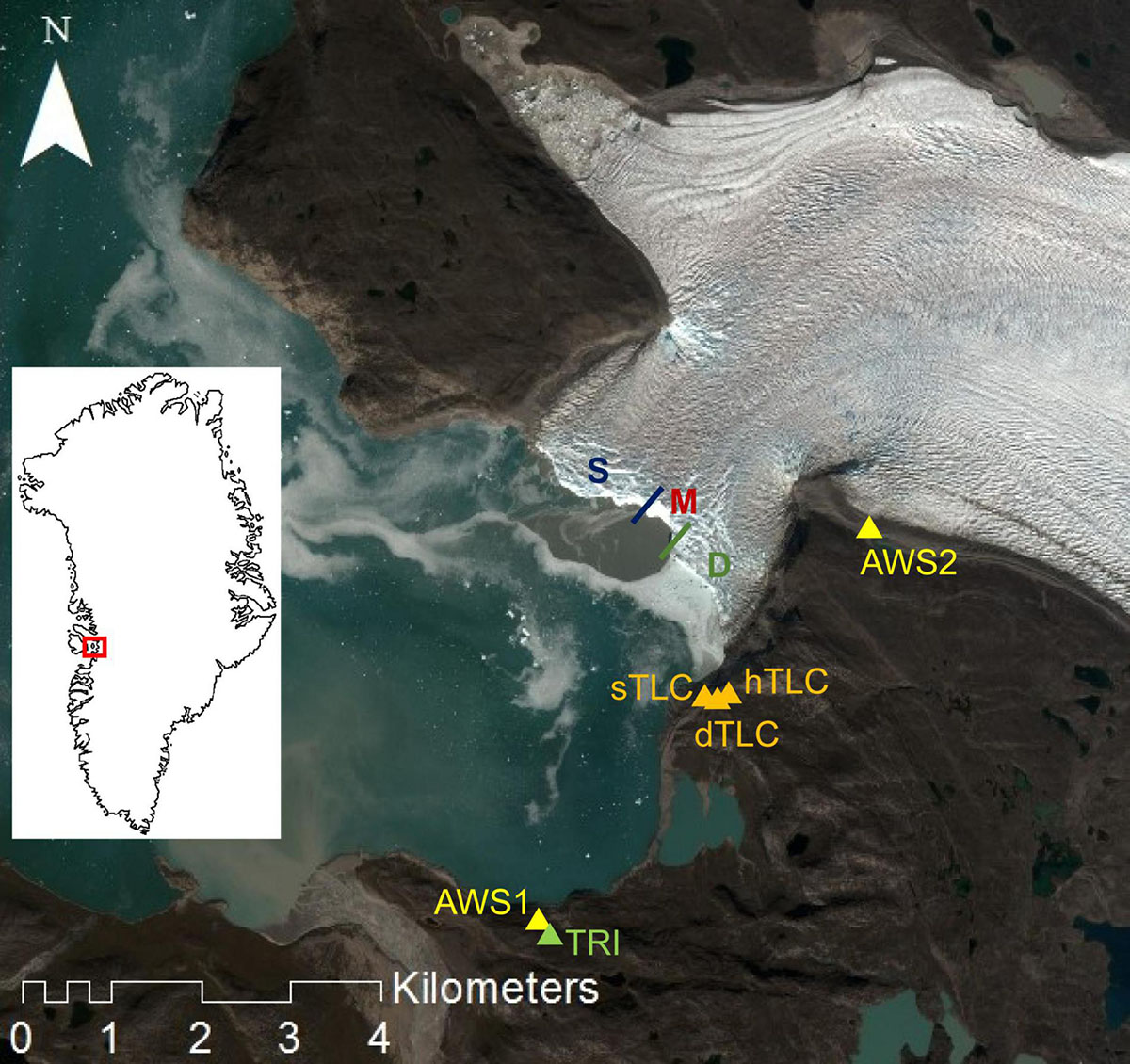
Figure 1. Overview of the field site at Eqip Sermia at the western margin of the Greenland ice sheet. The calving front can be separated in a shallow (S), a middle (M), and a deep sector (D). Background: Sentinel-2A scene from 3 August 2016 (from ESA Copernicus Science Hub: https://scihub.copernicus.eu). The positions of the terrestrial radar interferometer (TRI), the time-lapse cameras (hTLC, dTLC, sTLC) and the two weather stations (AWS1, AWS2) are indicated by triangles.
At Eqip Sermia a terrestrial radar interferometer (TRI, Gamma GPRI) was installed on bedrock 150 m above sea level at 4.5 km distance from the calving front (Figures 1, 2). The measurements were repeated at 1-min intervals during six field campaigns at different times in the ablation season (Supplementary Table 2). With these radar measurements an almost continuous record of velocity and elevation data was acquired during six field campaigns of 4–16 days duration (Supplementary Table 2).
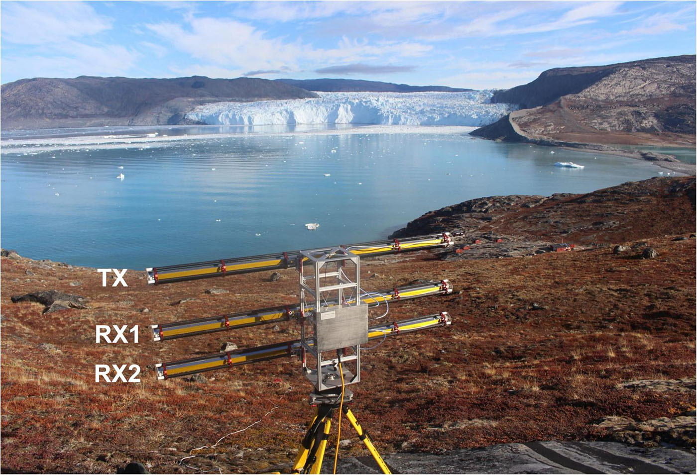
Figure 2. The terrestrial radar interferometer (TRI) with one transmitting (TX) and two receiving antennas (RX1, RX2) is located opposite of the front of Eqip Sermia at a distance of 4.5 km.
The Gamma GPRI is a real-aperture radar interferometer with one transmitting and two receiving antennas. The radar operates at a wavelength of λ = 17.4 mm (Ku-Band, 17.2 GHz). By calculating the interferograms between the two receiving antennas digital elevation models can be derived. Additionally, the velocity can be obtained by calculating interferograms with two consecutive images of one receiving antenna. The range resolution is approximately 0.75 m, while the azimuth resolution is 0.1 degrees corresponding to 7 m at a slant range of 4.5 km (Werner et al., 2008a).
Two automatic weather stations (AWS1, AWS2) collected hourly data at the sites indicated in Figure 1. AWS1 was installed near the TRI at 60 m a.s.l. and measured air temperature, relative humidity, wind, incoming shortwave radiation and precipitation. This station measured temperature from 2014 onward with several breaks in winter and spring due to insufficient power supply (Supplementary Figure 1). AWS2 located next to the ice edge at 362 m a.s.l. started to measure air temperature, radiation and wind in 2015 (Supplementary Figure 1). At AWS2 the meteorological conditions are influenced by the proximity of the ice sheet while AWS1 better represents the climate conditions at the shore of the fjord. Additionally, data of the station JAR 1 of the GCnet (Steffen et al., 1996) on the ice sheet at 962 m a.s.l. were used to estimate the environmental conditions during data gaps of AWS1 an AWS2.
Several time-lapse cameras (TLCs) were installed on the moraine next to the glacier front. From 2011 to 2020 a camera was taking pictures of the front once a day (dTLC; Kadded and Moreau, 2013). In 2017 an additional camera acquiring images at a 1-h interval (hTLC) was installed. During the field campaigns 2018 and 2019 a camera taking pictures every 10 seconds (sTLC) facilitated observing the glacier front and the calving process in more detail and with high temporal resolution. In 2018 this camera was installed from 8 July to 12 July, while in 2019 it was running from 16 August to 22 August (Supplementary Figure 1).
The TRI (GPRI) receives the radar signal with two antennas RX1 and RX2 (Figure 2), which facilitates topography reconstruction at a high temporal resolution. First, interferograms between RX1 and RX2 are calculated and unwrapped following the standard workflow described in Caduff et al. (2015). The unwrapped phases are then converted to topography (Strozzi et al., 2012), corrected for systematic errors (Walter et al., 2020) and the received topography afterward stacked over 10 min to reduce noise mainly caused by interferometric phase shifts due to changes in temperature, humidity, and air pressure (Goldstein, 1995). The obtained digital elevation models (DEMs) at intervals of 10 min have a resolution of 3.75 m in range (approximately the flow direction of the glacier), about 8 m in azimuth direction at the glacier front and show the height of the surface of the ice and the surroundings.
The successive processing steps of the TRI data follow the method described in detail in Walter et al. (2020), in which a DEM example is shown and an accuracy assessment of the final DEMs and calving volume detection is provided.
Calving events were detected by subtracting consecutive stacked DEMs and locating the negative elevation changes at the glacier front following the method presented in Walter et al. (2020). Due to the DEM stacking calving events within 10 min are merged together. Several thresholds to extract the calving events were used to reduce noise and to increase the signal-to-noise ratio on stable terrain. The calving events need a height change of more than 5 m, an area larger than 10 pixels (1 pixel ∼ 30 m2) and a width larger than 3 pixels (1 pixel ∼ 3.75 m). As noise patterns have mostly an irregular shape, events smaller than 40 pixels additionally have to fulfill the shape condition, which is (number of pixels × 1.6) ≥ [number of pixels in bounding box (max. extent in both directions)]. To exclude icebergs in the fjord and collapsing seracs upstream of the glacier front, a mask as a line with a buffer of about 75 m on each side of the front was used.
All calculations were done in the radar geometry and only the final results were resampled and reprojected into the cartesian UTM22N grid with nearest neighbor interpolation. Thus, errors due to resampling are independent of the earlier processing steps and do not influence the final findings.
Additionally to the DEMs, interferograms between consecutive radar images from the same receiver antenna were calculated to derive ice flow velocities. A stacking of 120 interferograms (2 h) before unwrapping the interferograms was used to reduce noise. The line-of-sight displacement was then calculated with the unwrapped interferograms (Werner et al., 2008b).
The daily time-lapse images from 2014 to 2017 and the hourly images from 2017 to 2019 were inspected visually. Thereby the geometric shape and position of the front were recorded manually to analyze the evolution of the front throughout the years. Additionally, the presence or absence of the mélange in the fjord and the submarine meltwater plumes emerging at the fjord surface were noted. For validation, several Sentinel 2 images were visually analyzed (from ESA Copernicus Science Hub: https://scihub.copernicus.eu).
The time-lapse images of sTLC, which acquired images in a 10-s interval during the field campaigns 2018 and 2019, were processed manually. The images were visually inspected to count and classify the calving events regarding the size, the source area and the calving type (example movie in Supplementary Material). For the source area the front was divided into seven sections shown in Figure 3. Sectors S1–S3 correspond roughly to the shallow sectors S and M and sectors D4–D7 to the deep sector D. Four magnitude classes were defined for the size, where magnitude 1 are very small events not causing any calving waves and magnitude 4 are large events causing calving waves that reach the shores opposite the calving front (see Figure 4 and Supplementary Figure 2 for examples). For the calving type we used the same classification as How et al. (2019) and assigned the calving events as ice-fall event (part of the ice breaking off from the subaerial front), sheet collapse (ice collapse with little or no rotation), stack topple (calving event rotates outward), subaqueous event (ice breaks off below the waterline and appears at the water surface) and waterline event (ice breaks off at the waterline) (see Figure 5 and Supplementary Figure 3 for examples). As the sTLC was looking on the glacier from the southern lateral moraine, large parts of the shallow sector S3 were only partly visible as the ice front was hidden behind a protruding spire. Sector M (Figure 1) is completely hidden and thus not analyzed separately but included in the shallow sector S3. Larger events behind the spire can produce a distinct water splash visible on the sTLC. These events are classified in magnitude and calving type as unknown. Behind sector S1 the glacier front would continue but is not in the field of view of the camera.

Figure 3. Calving front sectors used in time-lapse image analysis are marked with lines. The sectors S1–S3 of the front correspond to the shallow sectors S and M (blue; S1, S2, S3) and the sectors D4–D7 to the deep sector D (green; D4, D5, D6, D7). The middle sector is hidden and thus included in the shallow sector S3. The approximate subglacial meltwater plume locations are indicated and named P1–P4.
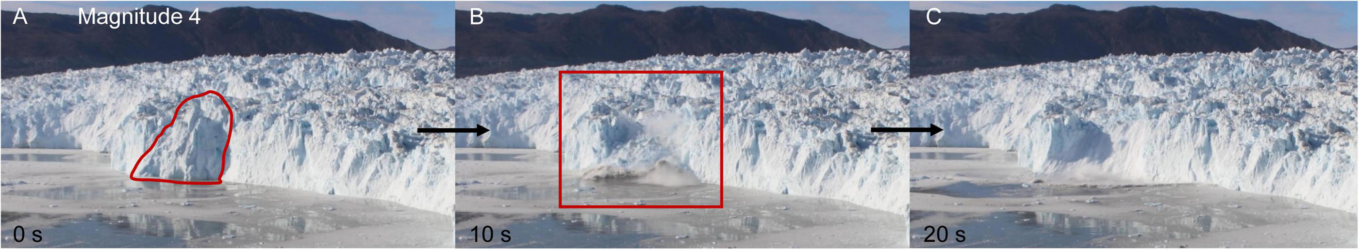
Figure 4. An example illustrating the definition of a magnitude 4 calving event for the sTLC images on 8 July 2018. The image sequence shows the example over time from 0 s (A) to 10 s (B) and 20 s (C). Examples of magnitude 1–3 are shown in Supplementary Figure 2.
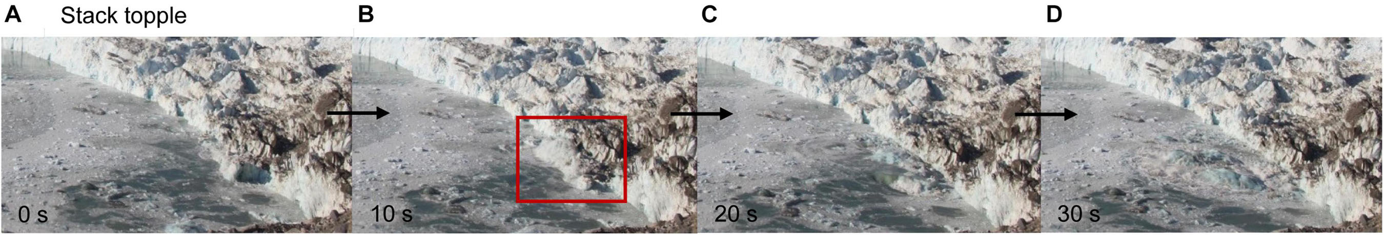
Figure 5. An example of the calving event type “stack topple” detected in the sTLC images on 8 July 2018. The image sequence shows the example over time from 0 s (A) to 10 s (B) 20 s (C) and 30 s (D). Examples of the other calving event types are shown in Supplementary Figure 3.
All three meteo stations AWS1, AWS2, and JAR1 used in this study show data gaps at different times (Supplementary Figure 1). To obtain an almost continuous temperature record the data of these stations were combined. If data from AWS2 was available, it was used directly. If no data from AWS2 but from AWS1 was available these values were corrected onto AWS2 with an offset of −1.55°C to account for a difference in elevation. If both AWS1 and AWS2 had a data gap values from JAR1 were modified with + 5.42°C (Rohner et al., unpublished). These offsets have been determined from substantial periods with data overlap. This resulted in an almost continuous record with only two data gaps in spring 2015 and 2016 (Supplementary Figure 16).
The 10 s time-lapse camera (sTLC) images from 2018 and 2019 campaigns allow a detailed analysis of the calving magnitudes and frequency at Eqip Sermia and a classification of calving styles. Examples of the magnitude classes are shown in Figure 4 and Supplementary Figure 2, while Figure 5 and Supplementary Figure 3 show examples of the different calving event types.
Figures 6, 7 and Supplementary Figures 5, 6, 7 show the results of the calving event type analysis over time and along the front. A total of 2038 calving events were detected during 3.8 days in July 2018, while in August 2019 during 6 days 2914 calving events were observed (Supplementary Table 1). This resulted in 536 events per day for 2018 and 480 events per day in 2019. In 2018 and 2019 most of the events were relatively small and of magnitude 1 and 2 and only 10% of all events were big (magnitude 3 or 4). In 2018 25% of all calving events were of the smallest magnitude 1 and did not cause calving waves, while in 2019 there were slightly less (20%). Events of magnitude 4 were with 1.9% in 2018 and 1.3% in 2019 rather rare.
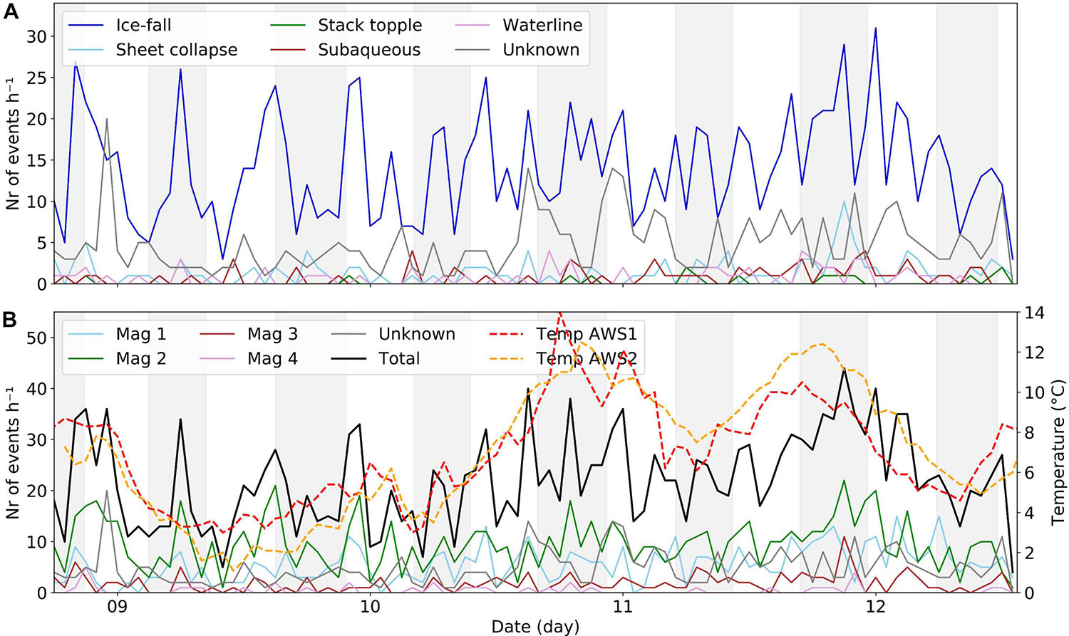
Figure 6. Calving event rates detected in the sTLC images over a 4 day period in July 2018. (A) Number of events per hour for the different calving types. (B) Number of events per hour for the different calving magnitudes. Air temperature from AWS1 and AWS2 is shown on the right axis. The gray background shading indicates rising tides.
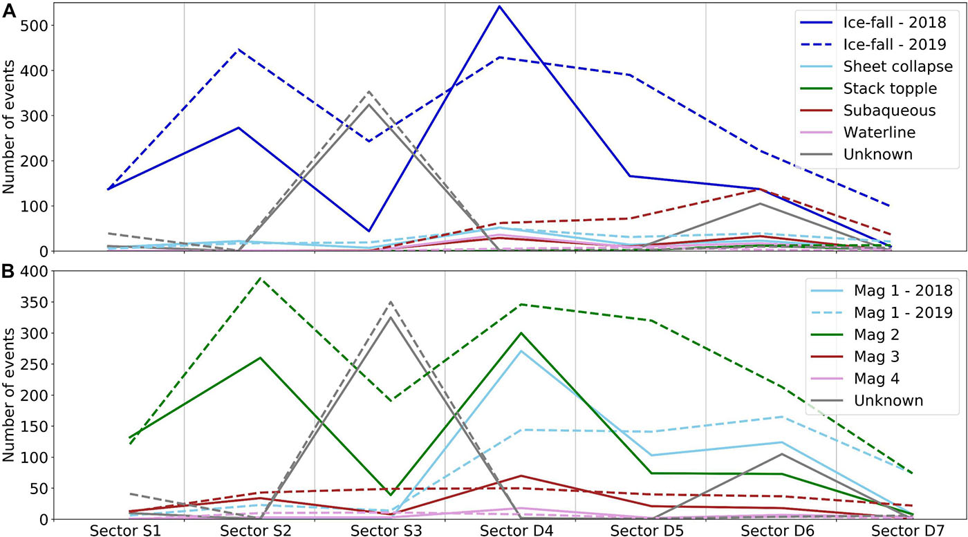
Figure 7. Number of events detected in the sTLC images (10s interval) for each calving front sector as defined in Figure 3 over a 4 day period in July 2018 (solid lines) and over a 6 day period in August 2019 (dashed lines), (A) for the calving types and (B) for the calving magnitudes.
Ice fall events were clearly the most frequent calving event type in both field campaigns 2018 and 2019 (64 and 67%, respectively). Subaqueous events were far less frequent and in 2019 contributed 11% compared with 4% in 2018 (Supplementary Table 1).
In Figure 7 type and magnitude of calving events along the calving front classified per sector are shown. While ice fall and sheet collapse events occurred in all sectors, stack topple, subaqueous and waterline events were almost exclusively observed in the deep sectors D4–D7. The highest diversity of event types was found in sector D6. During the field campaign 2018 sector D4 showed the most events, while in 2019 this was in sector S3, while most of these events occurred behind a protruding spire and were not visible with the time-lapse camera. These events were still counted and classified as unknown when a splash produced by the falling ice was observed. Sectors D4 and S3 also showed most events of magnitude 4.
In both years, strong temporal fluctuations in event frequency are observed from hour to hour for all calving magnitudes and styles, but no clear relationship with respect to diurnal temperature variations is apparent (Figure 6 and Supplementary Figures 5, 6, 7). However, during the field campaign 2018 an increasing trend in the number of events per hour occurred toward the end of the observation period (Figure 6B), whereby the increase was less strong for ice-fall events (Figure 6A). In parallel, air temperatures also showed an increasing trend. In contrast, in 2019 the rate of events was (besides short-term fluctuations) relatively constant during the entire observation period, but a shift from magnitude 1 to magnitude 2 was observable (Supplementary Figure 5). In both years no clear relationship with respect to the tides was observed. This was also the case if only the deep sector, which is more in contact with the ocean, is considered (Supplementary Figures 6, 7).
The evolution of the calving front was investigated using the daily time-lapse images for the years 2014–2017 and the hourly time-lapse images from 2017 to 2019. The front evolved every year in a similar manner starting with an advanced position in late winter, and a successive retreat throughout the melt period. Thus distinct states of the front were identified and the date when these states were present noted for every year (Figure 9). As an example the front evolution in 2018 is illustrated with time-lapse imagery in Figure 8.
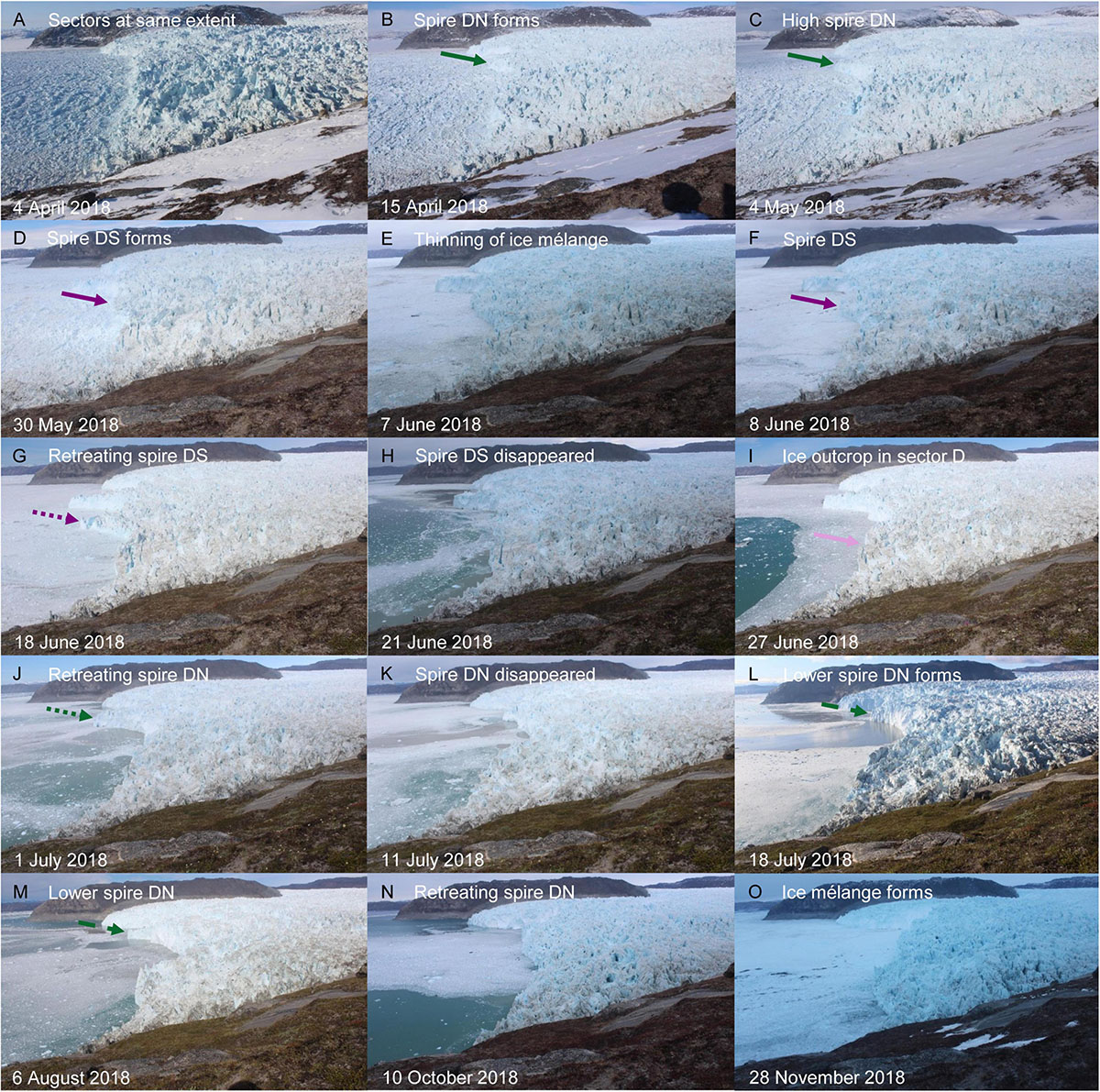
Figure 8. Calving front evolution during the year 2018 illustrated with selected hTLC images (A–O). The different colored arrows correspond to the states shown in Figure 9.

Figure 9. Calving front evolution throughout the year for 2014–2019 analyzed with hTLC and dTLC images. Important events and states in the calving front evolution are indicated, as well as periods of melting or freezing conditions, mélange cover and TRI field campaigns. Two spires form in the deep sector D, one in the northern sector D (DN) and one in the southern sector D (DS).
During winter the front advanced, whereby at a certain time in spring the different sectors all reached the same extent (Figure 8A). The location of the calving front became stable with the exception of the northern deep sector D (sector D4 in sTLC data), where the front continued to advance and a spire formed (spire DN; Figures 8B,C). In each year, this spire protruded strongly after a large calving event north of it, which was detectable from the time-lapse imagery. Additionally, in the southern sector D a second spire was observed (spire DS; Figures 8D,F). While the mélange was thinning a subglacial meltwater plume appeared a few days before the fjord became ice free at the same location where the first large calving event north of spire DN occurred. As soon as the plume was visible at the surface, the front retreated rapidly at this location due to large calving events. Elsewhere along the front, the calving activity increased when the ice mélange broke up, but caused only slight retreat (Figure 8E). More subglacial meltwater plumes appeared slightly after the first plume and always roughly at the same locations (Figure 3). The retreat of the front was substantially stronger at the locations of the subglacial meltwater plumes (Figures 8L, 10 and Supplementary Figure 9). Both spires started retreating in summer after the front at the plume locations on their sides retreated sufficiently. While spire DS disappeared at some point completely, spire DN sustained, although it became less high (Figure 8M). At the location of former spire DS, an ice outcrop appeared, which often was visible throughout the summer (Figure 8I). At the end of the summer season spire DN also retreated strongly and at the end of the year the mélange formed again (Figure 8O).
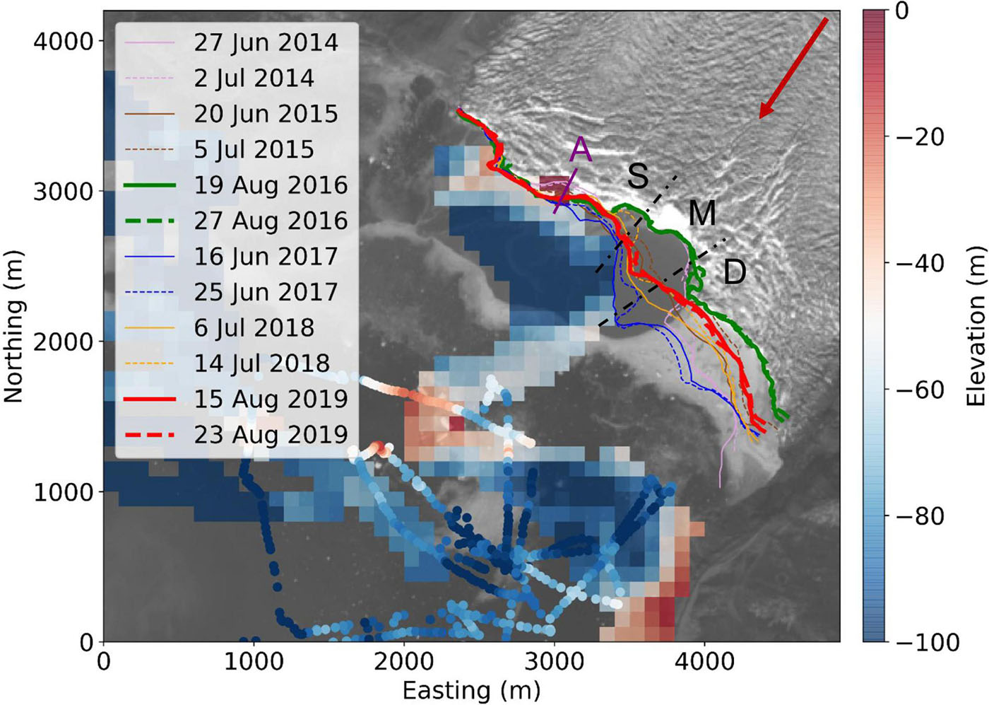
Figure 10. Position of the calving front at the beginning and the end of the TRI observation periods. The bed topography from depth soundings from a research vessel in 2014, 2015, and 2018 (Lüthi et al., 2016) are shown with circles and swath bathymetry data from Rignot et al. (2015) are shown as colored pixels. Note that no depth measurements exist directly below the glacier front. At the shallow sector bedrock was observed during low tide indicating a water depth of 0–20 m. The red arrow indicates the main flow direction of the glacier. Data from field campaigns later in the melt season (which typically have higher calving activity) are indicated by thick lines. At location A the slope over time was investigated (Supplementary Figure 12). Background: Sentinel-2A scene from 3 August 2016 (from ESA Copernicus Science Hub: https://scihub.copernicus.eu).
Comparing the evolution of the calving front during the years 2014–2019, Figure 9 shows that the mélange always disappeared more than a month after positive temperatures started, except in 2016, an exceptional year with early positive temperatures and an almost simultaneous ice mélange break-up. Further, in 2016 the front reached the same extent at all sectors earlier than in other years, which is in line with an early formation of the mélange in 2015. In 2015 and 2016 spire DN persisted throughout the summer until the mélange formed again. Spire DS retreated faster in the years 2018 and 2019 than before.
TRI observations were performed at different periods of the year (red shading in Figure 9) and consequently captured calving dynamics at different states in the seasonal cycle. In Supplementary Figure 4 the images of the front at the beginning and the end of all TRI observation periods are shown. While during the campaigns in 2014, 2015, and 2017 both spires DN and DS were present, in the other years the spire DS already disappeared. In 2015 and 2018 spire DN retreated during the TRI observations, while in 2016 and 2019 spire DN was already in its less high state. Overall, the TRI-campaigns from August 2016 and 2019 are much more representative of a late summer state of the calving front, whereas 2015, 2017, and 2018 refer rather to early melt-season and retreat onset.
The position of the calving front at the beginning and the end of the TRI observation periods are shown in Figure 10. It is clearly visible that the fluctuations of the front position were not homogenous along the front. Generally, the calving front was stable throughout the 6-years in the northern part of sector S, while in sectors D and M the front position varied substantially between the field campaigns. During the individual field campaigns the front was not changing considerably. The strongest retreats were observed during the field campaigns 2015 and 2018 in sector D (Supplementary Figure 9). The most advanced position was observed during the field campaign 2017, while the most retreated position was observed during the field campaign in August 2016.
The ice flow velocity along the front is presented in Figure 11A with speeds around 10 m per day for most parts of the front. The velocity was generally lower at the margins and showed two peaks with higher speed in sectors S and D. Highest velocities were observed during the field campaigns in July 2014, June 2015, and July 2018 (Figure 11A), while further upstream the velocity was clearly higher during the field campaign in July 2014 (Supplementary Figure 11A). During the observation period an increase in velocity especially in sector S occurred in 2015, 2017, and 2018 (Supplementary Figure 10A), which are field campaigns in early summer. In 2016 and 2019, with both observation periods late in the melt season, the velocity had a more decreasing trend or stayed constant (Supplementary Figures 10A, 21C). Both decreasing and increasing velocities were more significant at the southern part of sector S, at sector M and in the middle of sector D (Supplementary Figure 10A), where subglacial meltwater plumes appeared.
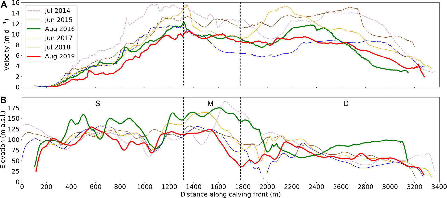
Figure 11. (A) Velocity and (B) elevation along the calving front during each field period as extracted from the TRI measurements. Data from field campaigns later in the melt season (which typically have higher calving activity) are indicated by thick lines.
In Figure 11B the elevation of the calving front for each individual field campaign is presented. The elevation of the calving front fluctuated strongly along the front due to the highly crevassed surface of the glacier. The elevation of the front was generally higher in sectors S and M than in sector D. During the field campaign 2016 with the most retreated front position, the front was higher than during the other field campaigns. Further upstream, the elevation in sector D was less high during the two late summer field campaigns in 2016 and 2019, while in sector S no clear pattern was observed (Supplementary Figure 11B). While during most observation periods no clear increasing or decreasing trend, comparing the beginning and the end of the observation period, was observable, in 2014 and 2015 the elevation increased significantly over time, mainly in sectors S and M (Supplementary Figure 10B). Additionally, the cliff shape was investigated over time at location A in sector S (Figure 10). The results in Supplementary Figure 12 show that during the field campaigns 2016 and 2019 the slope and shape of the front was constant, while during the other field campaigns the front evolved from a convex to a linear shape.
For the six field campaigns the positions and volumes of calving events were determined with the TRI data. To facilitate the comparison between the observation periods the numbers and volumes of calving events per day were calculated (Supplementary Table 2). The number of events per day ranged between 79 in 2015 and 149 in 2016, while the average calving volume per day was in between 1.8 × 10⁶ m3 and 2.6 × 10⁶ m3.
The detailed record of calving activity for all six field seasons is shown in Figures 12, 13. The main panels (Figures 12A,D,G, 13A,D,G) show the timing, position and color-coded volume of each calving event. The time resolution (horizontal bars) is 1 h and the spatial resolution 8 m. Clear patterns in space and time are immediately apparent, with active calving front sectors adjacent to sectors with rare, episodic, but large events. The changes in overall calving activity are shown as variations in number and volume per time interval in panels on the right of Figures 12, 13. Spatial variation of cumulative calving event volumes and numbers per day are shown in Figure 14.
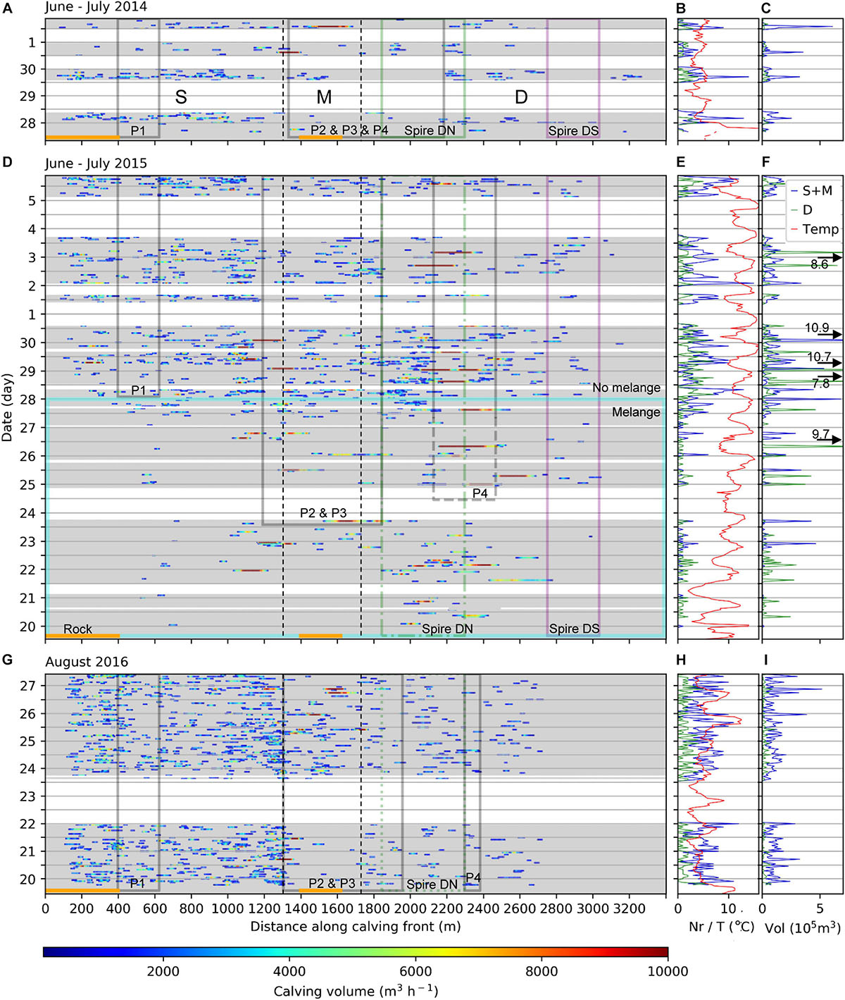
Figure 12. Calving event volumes along the front over time for the field campaigns in (A) 2014, (D) 2015, and (G) 2016. Calving volumes sampled during 1 h intervals are color coded. White areas indicate data gaps. The orange horizontal bars correspond to bedrock visible above the waterline. The gray boxes indicate the location and presence of meltwater plumes. Plumes P2, P3, and P4 can merge together. The black dotted vertical lines separate the sectors shallow (S), middle (M), and deep (D). The northern spire in sector D (DN) is indicated with a green box with a solid frame if the spire is still high, a dash-dotted frame if the spire is retreating and a dotted frame if the spire is in its low state (Figure 9). The southern spire in sector D (DS) is marked with a purple box. Number of events and temperature over time are shown in the middle panels for the field campaigns in (B) 2014, (E) 2015, and (H) 2016. The right panels show the volume of events over time for the field campaigns in (C) 2014, (F) 2015, and (I) 2016. Number and volume of calving events per hour are separated into the shallow (blue line, together with the middle) and deep sector (green line).
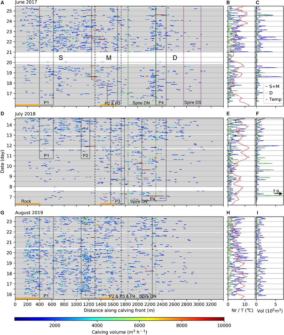
Figure 13. Same as Figure 12 but for the field campaigns in (A) 2017, (D) 2018 and (G) 2019.
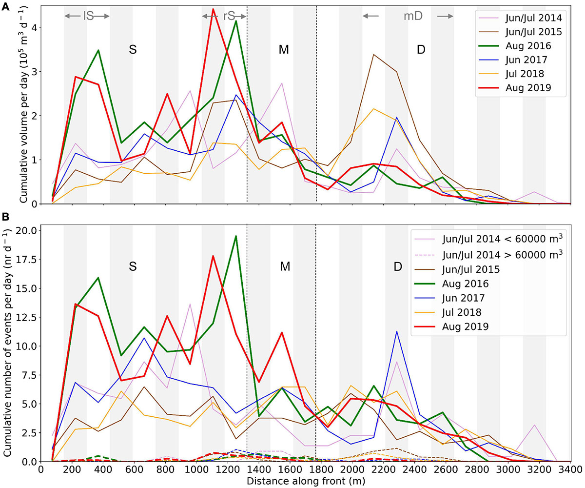
Figure 14. Cumulative (A) volume and (B) number of calving events per day along the front. The cumulative number of events per day are separated in smaller events with less than 60,000 m3 (solid lines) and large ones above 60,000 m3 (dotted lines). Data from field campaigns later in the melt season (which typically have higher calving activity) are indicated by thick lines.
Additional environmental information is also shown in the main panels of Figures 12, 13: The episodic occurrence of subglacial melt water plumes at different positions of the calving front, the presence of protruding ice spires, and bedrock visible at the calving front.
The calving patterns in Figures 12, 13 can be assigned to two different calving activity characteristics, from now on called high and reduced. The same observation can be made in Figure 14 showing the cumulative number and volume of events per day along the calving front. In general the observation periods with high calving activity were recorded later in the summer (2016, 2019) and showed many events throughout these observation periods (Figures 12G, 13G). This resulted in substantially higher numbers of events and volumes per day but mean and maximum calving event volumes actually decreased (Supplementary Table 2). Calving rates and volumes also differed between the three sectors, whereby in sector D substantially fewer (Figure 14) and also smaller calving events were detected (Supplementary Figure 14). Compared to sector S the middle sector showed also less but larger events (Figure 12G).
Reduced calving activity was recorded during observation periods at the beginning of the melt season (2015, 2017, 2018). These field campaigns showed a clear increase toward the end of the observation period (Figures 12, 13), particularly in sector S, where the increase is also rather abrupt with time. In sector D the number of calving events per day did, however, not vary much between the years (Figure 14B). During the field campaigns in 2015 and 2018 large events (above 60,000 m3) occurred in sector D (Figures 12D, 13D, 14B), which also caused larger mean event volumes per day (Supplementary Figure 14). 2017 was characterized by a concentrated occurrence of events in sector D at the same location as in 2015 and 2018 large events were observed (Figures 12, 13).
Comparing the field campaigns with high (2016, 2019) and reduced calving activity (other years) resulted in the largest differences regarding the volume per day in the southern part of sector S (rS), in the middle of Sector D (mD) as well as in the very shallow part (lS in Figure 14). Big events seemed to be constrained to the southern part of sector S (rS in Figure 14), where most events were detected, sector M and the middle of sector D (mD in Figure 14) and only rarely happening in other locations.
The field campaign 2015 showed a clear step increase on 27 June (Figure 12D) several weeks after the air temperatures became positive (Supplementary Figure 17). The time-lapse images show that on 27 June the mélange started to break-up and on 28 June the fjord was ice free. Simultaneously, rapidly enlarging subglacial meltwater plumes appeared in front of the calving face. Therefore, the days with and without mélange were analysed separately (Supplementary Table 3). For the first 8 days for the whole front 21.8 calving events per day were detected, whereby the rate was similar for sector S and D with 11.9 and 10.5 events per day, respectively. After the mélange was removed the calving frequency for the whole front increased immediately by a factor five to 99.7 events per day, with a higher increase for sector S (70.1 events per day) than for sector D (30.7 events per day) (Supplementary Table 3). While the number of events increased, the mean volume of the events almost halved.
During the campaigns of 2018 and 2019, both the TRI and the sTLC were recording simultaneously for 3.8 and 6 days, respectively, which provides the means of verifying the calving events detected with the TRI.
Calving events of magnitude 1 and many of magnitude 2 cannot be detected with the TRI as the volume is smaller than the detection thresholds. Further, subaqueous and waterline calving events as well as events in sector 7 (which is in the line-of-sight shadow) were not detected by the TRI. As the time-lapse camera sTLC was situated on the moraine next to the glacier, large parts of the shallow sector were not visible on the sTLC images.
Of the possible 265 and 491 common events in 2018, 2019, 72.5 and 72.9%, respectively, could be found in both data sets. This difference is mainly due to mostly small events at a protruding ice face or the lowest part of the ice face that were only detected by sTLC. Some 2.4% were found in the TRI data only and are likely false detections.
Overall, this comparison demonstrates that our TRI-analysis is able to detect most magnitude 3 and 4 events very well and provides a representative picture with regard to calving size and frequency.
The three air temperature data sets were rescaled to AWS2 using an offset correction factor, and provide an almost continuous air temperature series that is representative for the terminus area of Eqip Sermia (Rohner et al., unpublished). These data showed higher temperature variability during winter and spring season than during summer (Supplementary Figure 16). During winter and spring the temperature did only for a few days raise above 0°C. During summer the temperatures were more stable with values around 10–15°C. The temperatures became positive between beginning of April (2019) and mid of May (2018) (Supplementary Figure 17). Unfortunately, in 2016 and 2015 there are data gaps of about 1.5 months at the onset of the melting season, however, when comparing the different datasets it seems that 2016 was rather similar to 2019, while 2015 followed more the trend of 2017.
In Figure 15 the cumulative positive degree days are shown, which were calculated by adding up hourly positive temperatures. The early spring onset of 2019 is clearly visible, while the other years show a later but more abrupt initial increase in air temperature in the melting season. The timing of the first large calving event, the thinning of the ice mélange and the first subglacial meltwater plume differs up to 1 month for the individual years (Figure 15B).
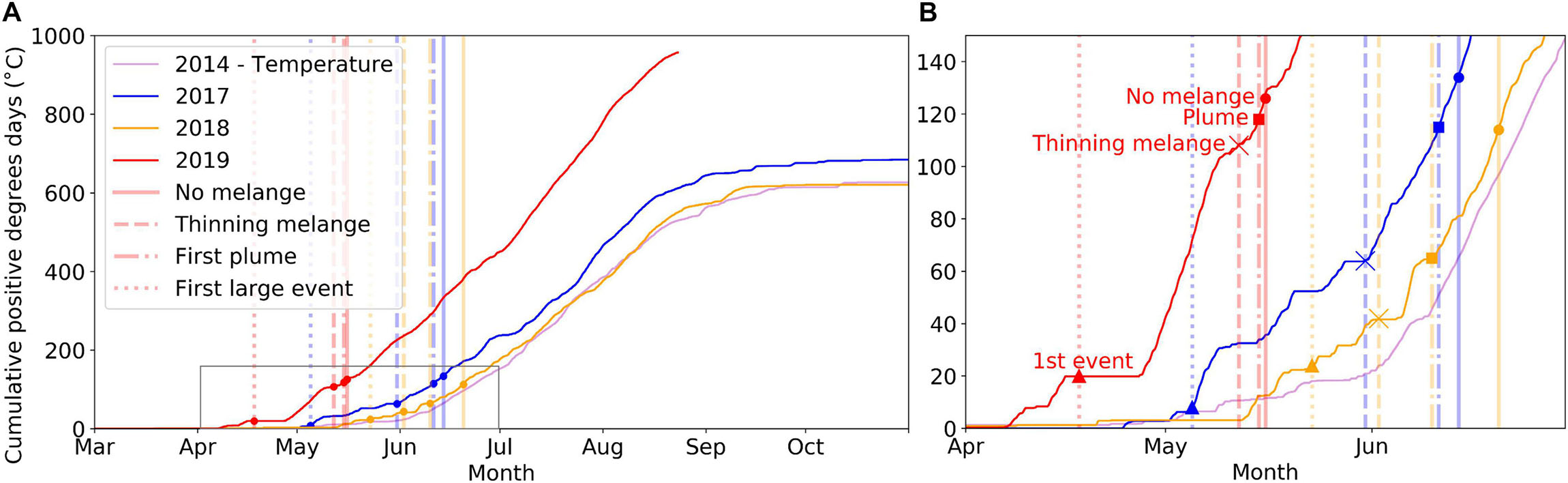
Figure 15. (A) Cumulative positive degree days calculated with the meteo data from AWS1, AWS2 and Jar1 for the elevation of AWS2 (360 m a.s.l.). (B) Enlargement of the gray square in A. The first large calving event occurred shortly after the temperatures became positive, while the first subglacial meltwater plume appeared at the sea surface only after some weeks of positive temperatures.
In general, our combined data indicates that the calving pattern and style depend on the calving front geometry and the formation of subglacial meltwater plumes and show a strong temporal variation throughout the summer. Notably, during the formation of subglacial meltwater plumes and related melt undercutting, striking changes in the pattern and frequency of calving with large events and a fast retreat of the front were observed. At locations with shallow bedrock the front advances further in winter and builds up two spires in the deep sector. Our calving observations suggest that later in the melt season subaquatic mass loss becomes more important and meltwater plumes turn out to be less important. In sector M the presence of a rock ridge stabilized the front (Walter et al., 2020) and large but less frequent events were observed when the front was in a strongly retreated position.
The field campaigns were undertaken during different states within the evolution of the front in the melt season, facilitating the observation of the various calving patterns and the investigation of the relevant processes and related forcings.
In the following we chronologically discuss the different states of the calving front and pattern through the season by integrating all datasets.
The calving front evolution follows a similar pattern in all 6-years of continuous time-lapse observations. This seasonal cycle is dominated by the fjord and bed topography and the subglacial discharge. Daily time-lapse imagery dTLC in Figure 8 illustrates frontal advance in winter, formation of meltwater plumes in spring, followed by rapid retreat and stabilization of the front position in summer. The exception is the northern half of the shallow sector S, which showed no clear advance or retreat as it is pinned on shallow bedrock (Figure 10 and Supplementary Figure 18) with substantially deeper water in front, preventing it to advance further. This stable front position in sector S is also clearly visible in Figure 10. The seasonal advance and retreat is a behavior commonly observed at tidewater glaciers in Greenland (Moon and Joughin, 2008; Howat et al., 2010; Schild and Hamilton, 2013; Fried et al., 2018).
In general, our data indicate that the timing of the different calving front states in the seasonal cycle depends on external drivers like air temperature and ocean currents. Figure 9 shows that the front reaches the same extent in all sectors between January and April, a few months before summer retreat starts. One month after air temperatures are above freezing and surface melt sets in, the ice mélange disintegrates. Some days earlier, a meltwater plume becomes visible at the same location where a large calving event reshaped the front significantly a few weeks earlier. At the positions of the plumes the front strongly retreats.
The strong influence of external drivers on the timing of the calving front states can be observed in exceptional years such as 2016, when record warm air and rain in April (NSIDC, 2016) lead to an almost simultaneous retreat of the ice mélange with first positive temperatures and hence a very early onset in retreat of the calving front.
After the fjord freezes over at the beginning of winter and the mélange forms, sectors M and D advance during 3 months. While ice mélange is present only very few calving events occur. Only when parts of the front reach deeper water (Figure 10 and Supplementary Figure 18) larger calving events happen (Supplementary Figure 20). The buttressing of the mélange seems to strongly suppress calving and consequently leads to the advance of the calving front. This behavior of front advance during the presence of mélange is also observed by satellite data for Eqip Sermia (Fried et al., 2018, Rohner et al., unpublished) and other tidewater outlet glaciers in western Greenland (Cassotto et al., 2015; Medrzycka et al., 2016), although at a lower temporal resolution.
The timing of the formation of ice mélange likely depends on both the air temperature and the heat content of the ocean. In 2014 and 2017 the freezing of the fjord was delayed due to above-average sea surface temperatures (Timmermans and Proshutinsky, 2015; Timmermans, 2016; Timmermans et al., 2017; Timmermans and Ladd, 2018, 2019). In contrast, in 2015 relatively low air temperatures (Overland et al., 2016) caused an earlier cover of mélange in the fjord.
After the fjord refreezes and the calving reduces, the front advances, except in the northern half of sector S, where the front position is constant since the bedrock drops significantly in flow direction (Figure 10; Rignot et al., 2015; Lüthi et al., 2016). This suggests that the water depth has an important influence on the advance of the glacier by influencing the mass loss at the front.
This observation is supported by the evolution of two spires in sector D as a re-occurring feature. These spires form on shallow bedrock during winter roughly 1 month after the front reaches the same extent in all sectors. While at the rest of the front ending in deeper water the ice flux and calving loss seem to balance, the two spires keep advancing (Supplementary Figure 18). Every year spire DN became a marked feature after the first large calving event north of it, which reshaped the front geometry significantly.
The yearly disintegration of the spires follows with a delay the retreat of the calving front as soon as the front at its sides retreated considerably. The delayed retreat is likely due to reduced undercutting by subglacial meltwater plumes, a process which caused considerable retreat in the areas next to the shallow bedrock (see section “Distinct Pattern of Early Seasonal Front Evolution and Calving During Growth of Meltwater Plumes”). In 2015 and 2018, the collapse of spire DN was captured in detail by the TRI-measurements and was related to several medium size calving events. In contrast, in 2017 the state was observed by TRI before the collapse and recorded a concentration of many mostly smaller calving events in sector D (Figure 13A, at 2,400 m). The spires thus influence the calving style as the higher front located on a rock bump led to more aerial events instead of subaquatic events.
Several weeks after the switch to positive temperatures and after a large calving event north of spire DN the ice mélange is thinning. During that time and shortly before the mélange disappears, the first subglacial meltwater plume appears at the same location where the large calving event was observed (Figure 12, meltwater plume P3). Simultaneously, the front starts to retreat strongly at this location (Supplementary Figure 22). Also the rest of sectors M and D start retreating slightly as soon as the mélange breaks up, similar to observations from other studies (Amundson et al., 2008; Joughin et al., 2008; Howat et al., 2010; Moon et al., 2015). In general our TRI-observations show a distinct step-increase in calving activity with the disappearance of the mélange (Figure 12D), which was also observed at Store glacier and KNS (Bunce et al., 2021; Cook et al., 2021). With this strong increase in calving events per day, the mean event size decreased. In sector D, the onset of retreat is characterized by larger events with full-thickness ice collapses. With the clearing away of the mélange additional subaquatic meltwater plumes become visible at the fjord surface. In general three plumes next to the two spires were observed, likely due to the focussing of subglacial meltwater discharge to deeper parts of the fjord (Truffer and Motyka, 2016). At the location of these meltwater plumes the front retreated significantly faster and to a more retreated position (Figure 10 and Supplementary Figure 9). Similar observations from 2013 to 2016 (Fried et al., 2018) were explained by subglacial meltwater plumes increasing retreat due to melt and undercutting (O’Leary and Christoffersen, 2013; Fried et al., 2015; Rignot et al., 2015; Slater et al., 2017).
Interestingly, during the growth of the meltwater plumes several large calving events exceeding 60,000 m3 occur and lead to a rapid retreat of the front. Such close links between plumes and big calving events can be observed in the early field seasons 2015 (plume P2 and P4), 2017 (plume P2) and 2018 (plume P4). As an example, during the field season 2017 with a generally reduced calving activity, large events occurred at plume P2, which formed a few days before the observations started and kept increasing in size. During 1 week several large calving events happened in the area of the plume and were likely triggered by melt undercutting.
Later in the summer the front position becomes stationary suggesting that the influence of meltwater plumes decreases. The calving activity becomes then independent of the presence of the meltwater plumes, as size and frequency of calving events are comparable to neighboring areas and the number of large calving events is significantly reduced. As the crevasses on the glacier surface are observed to be wider and deeper later in the season (Supplementary Figure 13), the ice is likely more damaged. Thus, smaller calving events become more frequent and the influence of melt undercutting, which leads to large events, decreases. During our TRI-observation periods large calving events solely occurred at locations expected to be influenced by meltwater plumes, with events exceeding 60,000 m3 only rarely outside of plume areas. This includes extreme events of up to 1,000,000 m3 that lead to large tsunami events (Lüthi et al., 2016).
At the beginning of the melt season (e.g., field campaigns 2015 and 2018), when meltwater production becomes substantial, the glacier is observed to accelerate, likely due to enhanced basal motion (Figure 11A and Supplementary Figure 21), a process also observed in other studies for Eqip Sermia (Lüthi et al., 2016; Rohner et al., unpublished). A rise in subglacial meltwater discharge is confirmed by the increasing size of meltwater plumes. The subglacial plume emergence often depends on the stratification in the fjord, but the shallow Eqip Sermia fjord might preclude a strong stratification, which allows to still use the subglacial meltwater plume as a proxy for subglacial discharge. The acceleration of sector S occurs simultaneously with a change in front geometry from a convex shape to a more linear but inclined cliff (Supplementary Figure 12). As soon as the inclined front formed, the calving activity in sector S increases, which was observed in both the TRI and the sTLC data. This suggests that in spring an acceleration of the ice flow first modifies the front geometry before calving shows a step increase, underlining the tight interactions between calving, front geometry and ice flow.
Later in the season the observations show lower and constant or slightly decreasing velocities (field campaigns 2016 and 2019; Figure 11A and Supplementary Figures 11A, 21C). Note that at this stage the air temperature, and hence the amount of meltwater, is similar to the early season. The decelerating velocities later in the season were likely due to a more efficient subglacial meltwater system. This has also been observed in other studies in western Greenland for tidewater glaciers (Moon et al., 2015) and for a land-terminating glacier with proxy measurements of subglacial water flow indicating a similar increase in hydraulic efficiency later in the melt season (Bartholomew et al., 2010). In the late melt season calving frequency in sector S is very high, but calving events are generally smaller. This is likely due to a strongly crevassed front as compared to spring (Supplementary Figure 13), which reduces the size of ice blocks and therefore leads to more but smaller calving events.
Late in the melt season the front position ceases to retreat and stabilizes at a constant position (example of front positions Supplementary Figure 22), despite continuing relatively warm atmospheric (and likely oceanic) conditions. We explain this by shallower water at this position. At this stage, and observed during the field campaigns 2016 and 2019, the ice flux and the mass loss seem to balance. When the calving front is in its retreated position the spatial calving pattern becomes clearly distinguishable for the different sectors of the front, with high calving activity in sector S and reduced activity in sector D. The reduced calving activity in sector D is likely due to higher volume loss by subaqueous calving and oceanic melt, possibly also causing smaller events, which cannot be detected with the TRI (Walter et al., 2020).
This suggestion is supported by the observation of varying calving types between the sectors. More specifically, subaqueous events solely occur in sector D and accounted for 19% of all events observed during the field campaign 2019, where the front was observed at a retreated position, compared to 2018 with only 6% subaqueous events as in sector D a plume was forming causing more full-thickness events. The percentage number of subaqueous events is still relatively small, but mass flux considerations by Walter et al. (2020) indicated that volume loss by subaqueous calving and oceanic melt account for up to 65%.
A unique data set of the outlet glacier Eqip Sermia, consisting of high-resolution terrestrial radar interferometry (TRI) data from six field campaigns, continuous daily and hourly time-lapse images over 6 years, and 10-s time-lapse images of two field campaigns enabled a detailed analysis of the evolution of the calving front and the calving process. High temporal resolution calving event volume catalogs were obtained with the TRI by differencing the calculated elevation models and extracting negative elevation changes. The continuous time-lapse images from 2014 to 2019 facilitated the interpretation of the different patterns of the TRI-derived calving events within the seasonal cycle, while the 10-s time-lapse images served as validation data and provided information on variations in calving type.
We found that the calving pattern and style of Eqip Sermia was diverse for the sections of the calving front with different geometry and varied strongly throughout the year depending on the state in the seasonal cycle of the calving front and the related environmental conditions. The temporal and spatial evolution of the calving front was observed to be controlled by the bed and fjord topography and the emergence of subglacial meltwater plumes. Short term variations in air temperature or tides seem to have no direct influence on calving activity. During the formation of surface melt induced plumes, starting a few days before the ice mélange disappears, an immediate and strong increase in calving activity was observed (frequency and flux). This further triggered large calving events likely due to undercutting and as a consequence, the front retreated stronger and faster at locations of these plumes. Large calving events exceeding 60,000 m3 were rarely observed outside of areas influenced by a plume. Later in the melt season the calving activity at subglacial meltwater plumes is similar to the neighboring areas, suggesting the presence of plumes to become less important for calving. At locations of shallow water the front advanced further during winter, forming two spires as striking elements of the front. These spires retreated with a delay and disintegrated when the front either side of it retreated considerably. Later in the season the front position became stationary again and the flow velocity decelerated. At this state the calving patterns between the different sectors became clearly distinguishable with frequent smaller events in the shallow sector S and reduced calving activity in sector D, where subaqueous mass loss consisting of submarine calving and oceanic melt is expected to become dominant.
This study shows that the combination of different measurement techniques is important to overcome their individual limitations and to investigate calving and the forcings leading to iceberg detachment. The results demonstrate a high temporal variability of calving frequency, size and flux and a strong dependence of calving and front evolution on bed and fjord topography and on the formation of meltwater plumes. These plumes are fed by subglacial discharge and hence are indirectly coupled to atmospheric forcing.
Our observations highlight the complexity and temporal variability of calving and its interactions with environmental forcing. Therefore, long-term and high temporal resolution observations of calving are needed to test and further develop calving models, which are key to understand the dynamics of outlet glaciers at present and in the future.
A time-lapse movie of Eqip Sermia with hourly images from 2017 to 2019, two calving event catalogs determined with the 10-s time-lapse images during the field campaigns 2018 and 2019 and the meteorological data of two weather stations are available from https://doi.org/10.5281/zenodo.4700651. Another time-lapse movie with daily images from 2012 to 2015 is available from https://www.youtube.com/watch?v=26vaXqJpvyE. The TRI data are available upon request from the authors.
AK-W, ML, and AV designed the study and carried out the field work. AK-W performed all analysis and wrote the draft of the manuscript. LM maintained the daily time-lapse cameras and provided the images for analysis. All authors contributed to the final version of the manuscript.
This work was funded by the Forschungskredit of the University of Zurich (grant no. FK-19-090) and the University of Zurich and the ETH Zurich, Switzerland. The field work was supported through Swiss National Science Foundation (grant nos. 200021-156098 and 200021-153179/1).
The authors declare that the research was conducted in the absence of any commercial or financial relationships that could be construed as a potential conflict of interest.
We thank Christoph Rohner, Rémy Mercenier, Guillaume Jouvet, Eef van Dongen and all the 3G master students for help during the field campaigns at Eqip Sermia. A special thank goes to Diego Wasser, who developed and installed the time-lapse cameras running since 2017. We acknowledge the reviews by the three reviewers AS, TC, and LS and the comments by the scientific editor AH, which improved the manuscript.
The Supplementary Material for this article can be found online at: https://www.frontiersin.org/articles/10.3389/feart.2021.667717/full#supplementary-material
Amundson, J. M., Clinton, J. F., Fahnestock, M., Truffer, M., Lüthi, M. P., and Motyka, R. J. (2012). Observing calving generated ocean waves with coastal broadband seismometers, Jakobshavn Isbræ, Greenland. Ann. Glaciol. 53, 79–84. doi: 10.3189/2012/AoG60A200
Amundson, J. M., Truffer, M., Lüthi, M. P., Fahnestock, M., West, M., and Motyka, R. J. (2008). Glacier, fjord, and seismic response torecent large calving events, Jakobshavn Isbræ, Greenland. Geo-Phys. Res. Lett. 35:L22501. doi: 10.1029/2008GL035281
Bamber, J. L., Westaway, R. M., Marzeion, B., and Wouters, B. (2018). The land ice contribution to sea level during the satellite era. Environ. Res. Lett. 13:063008. doi: 10.1088/1748-9326/aac2f0
Bartholomaus, T. C., Larsen, C. H. F., O’Neel, S., and West, M. E. (2012). Calving seismicity from iceberg-sea surface interactions. J. Geophys. Res. 117:F04029. doi: 10.1029/2012JF002513
Bartholomaus, T. C., Larsen, C. H. F., West, M. E., O’Neel, S., Pettit, E. C., and Truffer, M. (2015). Tidal and seasonal variations in calving flux observed with passive seismology. J. Geophys. Res.-Earth Surf. 120, 2318–2337. doi: 10.1002/2015JF003641
Bartholomew, I., Nienow, P., Mair, D., Hubbard, A., King, M. A., and Sole, A. (2010). Seasonal evolution of subglacial drainage and acceleration in a Greenland outlet glacier. Nat. Geosci. 3, 408–411. doi: 10.1038/NGEO863
Benn, D. I., Warren, C. R., and Mottram, R. H. (2007). Calving processes and the dynamics of calving glaciers. Earth-Sci. Rev. 82, 143–179. doi: 10.1016/j.earscirev.2007.02.002
Bunce, C., Nienow, P., Sole, A., Cowton, T., and Davison, B. (2021). Influence of glacier runoff and near-terminus subglacial hydrology on frontal ablation at a large Greenlandic tidewater glacier. J. Glaciol. 67, 343–352. doi: 10.1017/jog.2020.109
Caduff, R., Schlunegger, F., Kos, A., and Wiesmann, A. (2015). A review of terrestrial radar interferometry for measuring surface change in the geosciences. Earth Surf. Process. Landf. 40, 208–228. doi: 10.1002/esp.3656
Cassotto, R., Fahnestock, M., Amundson, J. M., Truffer, M., Boettcher, M. S., de la Pena, S., et al. (2018). Non-linear glacier response to calving events, Jakobshavn Isbræ, Greenland. J. Glaciol. 4, 1–16. doi: 10.1017/jog.2018.90
Cassotto, R., Fahnestock, M., Amundson, J. M., Truffer, M., and Joughin, I. (2015). Seasonal and interannual variations in ice melange rigidity and its impact on terminus stability, Jakobshavn Isbrae, Greenland. J. Glaciol. 61, 76–88. doi: 10.3189/2015JoG13J235
Chapuis, A., Rolstad, C., and Norland, R. (2010). Interpretation of amplitude data from a ground-based radar in combination with terrestrial photogrammetry and visual observations for calving monitoring of Kronebreen, Svalbard. Ann. Glaciol. 51, 34–40. doi: 10.3189/172756410791392781
Cook, S., Christoffersen, P., Truffer, M., Chudley, T. R., and Abellan, A. (2021). Calving of a large Greenlandic tidewater glacier has complex links to meltwater plumes and mélange. J. Geophys. Res.: Earth Surface 126:e2020JF006051. doi: 10.1029/2020JF006051
Enderlin, E. M., Howat, I. M., Jeong, S., Noh, M.-J., van Angelen, J. H., and van den Broeke, M. R. (2014). An improved mass budget for the Greenland ice sheet. Geophys. Res. Lett. 41, 866–872. doi: 10.1002/2013GL059010
Fried, M. J., Catania, G. A., Bartholomaus, T. C., Duncan, D., Davis, M., Stearns, L. A., et al. (2015). Distributed subglacial discharge drives significant submarine melt at a Greenland tidewater glacier. Geophys. Res. Lett. 42, 9328–9336. doi: 10.1002/2015GL065806
Fried, M. J., Catania, G. A., Stearns, L. A., Sutherland, D. A., Bartholomaus, T. C., Shroyer, E., et al. (2018). Reconciling drivers of seasonal terminus advance and retreat at 13 central west Greenland tidewater glaciers. J. Geophys. Res.: Earth Surface 123, 1590–1607. doi: 10.1029/2018JF004628
Glowacki, O., Deane, G. B., Moskalik, M., Blondel, P. H., Tegowski, J., and Blaszczyk, M. (2015). Underwater acoustic signatures of glacier calving. Geophys. Res. Lett. 42, 804–812. doi: 10.1002/2014GL062859
Goldstein, R. (1995). Atmospheric limitations to repeat-track radar interferometry. Geophys. Res. Lett. 22, 2517–2520. doi: 10.1029/95GL02475
How, P., Schild, K. M., Benn, D. I., Noormets, R., Kirchner, N., and Luckman, A. (2019). Calving controlled by melt-under-cutting: detailed calving styles revealed through time-lapse observations. Ann. Glaciol. 60, 20–31. doi: 10.1017/aog.2018.28
Howat, I. M., Box, J. E., Ahn, Y., Herrington, A., and McFadden, E. M. (2010). Seasonal variability in the dynamics of marine-terminating outlet glaciers in Greenland. J. Glaciol. 56, 601–613.
Joughin, I., Abdalati, W., and Fahnestock, M. (2004). Large fluctuations in speed on Greenland’s Jakobshavn Isbrae glacier. Nature 432, 608–610. doi: 10.1038/nature03130
Joughin, I., Howat, I. M., Fahnestock, M., Smith, B., Krabill, W., Alley, R. B., et al. (2008). Continued evolution of Jakobshavn Isbrae following its rapid speedup. J. Geophys. Res. 113:F04006. doi: 10.1029/2008JF001023
Jouvet, G., Weidmann, Y., Seguinot, J., Funk, M., Abe, T., Sakakibara, D., et al. (2017). Initiation of a major calving event on the Bowdoin Glacier captured by UAV photogrammetry. Cryosphere 11, 911–921. doi: 10.5194/tc-11-911-2017
Jouvet, G., Weidmann, Y., van Dongen, E., Lüthi, M. P., Vieli, A., and Ryan, J. C. (2019). High-endurance UAV for monitoring calving glaciers: application to the inglefield bredning and Eqip Sermia, Greenland. Front. Earth Sci. 7:206. doi: 10.3389/feart.2019.00206
Kadded, F., and Moreau, L. (2013). Sur les traces de Paul-Emile Victor, relevés topographiques 3d au Groenland. Revue Leica XYZ 137, 47–56.
King, M. D., Howat, I. M., Candela, S. G., Noh, M. J., Jeong, S., Noël, B. P. Y., et al. (2020). Dynamic ice loss from the Greenland Ice Sheet driven by sustained glacier retreat. Commun. Earth Environ. 1:1. doi: 10.1038/s43247-020-0001-2
Köhler, A., Nuth, C. H., Kohler, J., Berthier, E., Weidle, C. H., and Schweitzer, J. (2016). A 15 year record of frontal glacier ablation rates estimated from seismic data. Geophys. Res. Lett. 43, 12155–12164. doi: 10.1002/2016GL070589
Köhler, A., Petlicki, M., Lefeuvre, P.-M., Buscaino, G., Nuth, C., and Weidle, C. (2019). Contribution of calving to frontal ablation quantified from seismic and hydroacoustic observations calibrated with lidar volume measurements. Cryosphere 13, 3117–3137. doi: 10.5194/tc-13-3117-2019
Lüthi, M. P., and Vieli, A. (2016). Multi-method observation and analysis of a tsunami caused by glacier calving. Cryosphere 10, 995–1002. doi: 10.5194/tc-10-995-2016
Lüthi, M. P., Vieli, A., Moreau, L., Joughin, I. R., Reisser, M., Small, D., et al. (2016). A century of geometry and velocity evolution at Eqip Sermia, West Greenland. J. Glaciol. 62, 640–654. doi: 10.1017/jog.2016.38
Medrzycka, D., Benn, D. I., Box, J. E., Copland, L., and Balog, J. (2016). Calving behavior at Rink Isbræ, West Greenland, from time-lapse photos. Arctic Antarctic Alpine Res. 48, 263–277. doi: 10.1657/AAAR0015-059
Minowa, M., Podolskiy, E. A., Jouvete, G., Weidmanne, Y., Sakakibara, D., and Tsutaki, S. (2019). Calving flux estimation from tsunami waves. Earth and Planetary Sci. Lett. 515, 283–290. doi: 10.1016/j.epsl.2019.03.023
Minowa, M., Podolskiy, E. A., Sugiyama, S., Sakakibara, D., and Skvarca, P. (2018). Glacier calving observed with time-lapse imagery and tsunami waves at Glaciar Perito Moreno, Patagonia. J. Glaciol. 64, 62–376. doi: 10.1017/jog.2018.28
Moon, T., and Joughin, I. (2008). Changes in ice front positions on Greenland’s outlet glaciers from 1992 to 2007. J. Geophys. Res. 113:F02022. doi: 10.1029/2007JF000927
Moon, T., Joughin, I., and Smith, B. E. (2015). Seasonal to multiyear variability of glacier surface velocity, terminus position, and sea ice/ice mélange in northwest Greenland. J. Geophys. Res.: Earth Surface 120, 818–833. doi: 10.1002/2015JF003494
Nick, F. M., Vieli, A., Howat, I. M., and Joughin, I. (2009). Large-scale changes in Greenland outlet glacier dynamics triggered at the terminus. Nat. Geosci. 2, 110–114. doi: 10.1038/ngeo394
NSIDC (2016). Early Start to Greenland Ice Sheet melt season, Greenland Ice Sheet Today. Available online at: http://nsidc.org/greenland-today/2016/04/early-start-to-greenland-ice-sheet-melt-season (accessed 11 November 2020).
O’Leary, M., and Christoffersen, P. (2013). Calving on tidewater glaciers amplified by submarine frontal melting. Cryosphere 7, 119–128. doi: 10.5194/tc-7-119-2013
O’Neel, S., Echelmeyer, K. A., and Motyka, R. J. (2003). Shortterm variations in calving of a tidewater glacier. LeConte Glacier, Alaska, U.S.A. J. Glaciol. 49, 587–598. doi: 10.3189/172756503781830430
O’Neel, S., Larsen, C. H. F., Rupert, N., and Hansen, R. (2010). Iceberg calving as a primary source of regional-scale glacier-generated seismicity in the St. Elias Mountains, Alaska. J. Geophys. Res. 115:L22501. doi: 10.1029/2009JF001598
Overland, J., Hanna, E., Hanssen-Bauer, I., Kim, S.-J., Walsh, J. E., Wang, M., et al. (2016). Surface Air Temperature [in Arctic Report Card 2016]. Available online at: http://www.arctic.noaa.gov/Report-Card (accessed 1 October 2020).
Petlicki, M., and Kinnard, C. H. (2016). Calving of Fuerza Aérea Glacier (Greenwich Island, Antarctica) observed with terrestrial laser scanning and continuous video monitoring. J. Glaciol. 62, 835–846. doi: 10.1017/jog.2016.72
Podgórski, J., Pȩtlicki, M., and Kinnard, C. (2018). Revealing recent calving activity of a tidewater glacier with terrestrial LiDAR reflection intensity. Cold Regions Sci. Technol. 151, 288–301. doi: 10.1016/j.coldregions.2018.03.003
Rignot, E., Fenty, I., Xu, Y., Cai, C., and Kemp, C. (2015). Undercutting of marine-terminating glaciers in West Greenland. Geophys. Res. Lett. 42, 5909–5917. doi: 10.1002/2015GL064236
Rolstad, C., and Norland, R. (2009). Ground-based interferometric radar for velocity and calving-rate measurements of the tidewater glacier at Kronebreen, Svalbard. Ann. Glaciol. 50, 47–54. doi: 10.3189/172756409787769771
Ryan, J. C., Hubbard, A. L., Box, J. E., Todd, J., Christoffersen, P., Carr, J. R., et al. (2015). UAV photogrammetry and structure from motion to assess calving dynamics at Store Glacier, a large outlet draining the Greenland ice sheet. Cryosphere 9, 1–11. doi: 10.5194/tc-9-1-2015
Schild, K. M., and Hamilton, G. S. (2013). Seasonal variations of outlet glacier terminus position in Greenland. J. Glaciol. 59, 759–770. doi: 10.3189/2013JoG12J238
Slater, D., Nienow, P. W., Goldberg, D. N., Cowton, T. R., and Sole, A. J. (2017). A model for tidewater glacier undercutting by submarine melting. Geophys. Res. Lett. 44, 2360–2368. doi: 10.1002/2016GL072374
Steffen, K., Box, J. E., and Abdalati, W. (1996). Greenland Climate Network: GC-Net. In: S. C. Ed. CRREL 96-27 Special Report on Glaciers, Ice Sheets and Volcanoes, trib. to M. Meier, S. Newark, NJ: 98–103.
Strozzi, T., Werner, C., Wiesmann, A., and Wegmüller, U. (2012). Topography mapping with a portable real-aperture radar interferometer. IEEE Geosci. Remote Sens. Lett. 9, 277–281. doi: 10.1109/LGRS.2011.2166751
The Imbie Team, Shepherd, A., and Ivins, E. (2020). Mass balance of the Greenland Ice Sheet from 1992 to 2018. Nature 579, 233–239. doi: 10.1038/s41586-019-1855-2
Thomas, R. H. (2004). Force-perturbation analysis of recent thinning and acceleration of Jakobshavn Isbræ, Greenland. J. Glaciol. 50, 57–66. doi: 10.3189/172756504781830321
Timmermans, M.-L. (2016). Sea Surface Temperature [in Arctic Report Card 2016]. Available online at: http://www.arctic.noaa.gov/Report-Card (accessed 1 October 2020).
Timmermans, M.-L., and Ladd, C. (2018). Sea Surface Temperature [in Arctic Report Card 2018]. Available online at: http://www.arctic.noaa.gov/Report-Card (accessed 1 October 2020).
Timmermans, M.-L., and Ladd, C. (2019). Sea Surface Temperature [in Arctic Report Card 2019]. Available online at: http://www.arctic.noaa.gov/Report-Card (accessed 1 October 2020).
Timmermans, M.-L., Ladd, C., and Wood, K. (2017). Sea Surface Temperature [in Arctic Report Card 2017]. Available online at: http://www.arctic.noaa.gov/Report-Card (accessed 1 October 2020).
Timmermans, M.-L., and Proshutinsky, A. (2015). Sea Surface Temperature [in Arctic Report Card 2015]. Available online at: http://www.arctic.noaa.gov/Report-Card (accessed 1 October 2020).
Truffer, M., and Motyka, R. J. (2016). Where glaciers meet water: subaqueous melt and its relevance to glaciers in various settings. Rev. Geophys. 54, 220–239. doi: 10.1002/2015RG000494
Vallot, D., Adinugroho, S., Strand, R., How, P., Pettersson, R., Benn, D. I., et al. (2019). Automatic detection of calving events from time-lapse imagery at Tunabreen, Svalbard, Geosci. Instrum. Method. Data Syst. 8, 113–127. doi: 10.5194/gi-8-113-2019
Van den Broeke, M. R., Enderlin, E. M., Howat, I. M., Munneke, P. K., Noël, B. P. Y., van de Berg, W. J., et al. (2016). On the recent contribution of the Greenland ice sheet to sea level change. Cryosphere 10, 1933–1946. doi: 10.5194/tc-10-1933-2016
Voytenko, D., Stern, A., Holland, D. M., Dixon, T. H., Christianson, K., and Walker, R. T. (2015). Tidally driven ice speed variation at Helheim Glacier, Greenland, observed with terrestrial radar interferometry. J. Glaciol. 61, 301–308. doi: 10.3189/2015JoG14J173
Walter, A., Lüthi, M. P., and Vieli, A. (2020). Calving event size measurements and statistics of Eqip Sermia, Greenland, from terrestrial radar interferometry. Cryosphere 14, 1051–1066. doi: 10.5194/tc-14-1051-2020
Walter, F., Olivieri, M., and Clinton, J. F. (2013). Calving event detection by observation of seiche effects on the Greenland fjords. J. Glaciol. 59, 162–178. doi: 10.3189/2013JoG12J118
Walter, F., O’Neel, S., McNamara, D., Pfeffer, W. T., Bassis, J. N., and Fricker, H. A. (2010). Iceberg calving during transition from grounded to floating ice. Columbia Glacier, Alaska. Geophys. Res. Lett. 37:L15501. doi: 10.1029/2010GL043201
Warren, C. R., Glasser, N. F., Harrison, S., Winchester, V., Kerr, A. R., and Rivera, A. (1995). Characteristics of tide-water calving at Glaciar San Rafael, Chile. J. Glaciol. 41, 273–289. doi: 10.3189/S0022143000016178
Werner, C., Strozzi, T., Wiesmann, A., and Wegmüller, U. (2008a). “A Real-aperture radar for ground-based differential interferometry,” in Proceeding of the IGARSS Conference Paper, (IEEE), 210–213.
Werner, C., Strozzi, T., Wiesmann, A., and Wegmüller, U. (2008b). “Gamma’s portable radar interferometer,” in Proceeding of the 13th FIG Symposium on Deformation Measurment and Analysis, (Research Gate).
Xie, S., Dixon, T. H., Holland, D. M., Voytenko, D., and Vanková, I. (2019). Rapid iceberg calving following removal of tightly packed pro-glacial mélange. Nat. Commun. 10:3250. doi: 10.1038/s41467-019-10908-4
Keywords: calving glaciers, calving, tidewater glacier dynamics, terrestrial radar interferometer, time-lapse imagery, meltwater plumes, mélange
Citation: Kneib-Walter A, Lüthi MP, Moreau L and Vieli A (2021) Drivers of Recurring Seasonal Cycle of Glacier Calving Styles and Patterns. Front. Earth Sci. 9:667717. doi: 10.3389/feart.2021.667717
Received: 14 February 2021; Accepted: 23 April 2021;
Published: 28 May 2021.
Edited by:
Alun Hubbard, Aberystwyth University, United KingdomReviewed by:
Andrew John Sole, The University of Sheffield, United KingdomCopyright © 2021 Kneib-Walter, Lüthi, Moreau and Vieli. This is an open-access article distributed under the terms of the Creative Commons Attribution License (CC BY). The use, distribution or reproduction in other forums is permitted, provided the original author(s) and the copyright owner(s) are credited and that the original publication in this journal is cited, in accordance with accepted academic practice. No use, distribution or reproduction is permitted which does not comply with these terms.
*Correspondence: Andrea Kneib-Walter, YW5kcmVhLndhbHRlckBnZW8udXpoLmNo
Disclaimer: All claims expressed in this article are solely those of the authors and do not necessarily represent those of their affiliated organizations, or those of the publisher, the editors and the reviewers. Any product that may be evaluated in this article or claim that may be made by its manufacturer is not guaranteed or endorsed by the publisher.
Research integrity at Frontiers
Learn more about the work of our research integrity team to safeguard the quality of each article we publish.