 Mohammad Hanif Hamden1
 Ami Hassan Md Din1,2*Dudy Darmawan Wijaya3Mohd Yunus Mohd Yusoff4Muhammad Faiz Pa’suya5
- 1Geospatial Imaging and Information Research Group (GI2RG), Faculty of Built Environment and Surveying, Universiti Teknologi Malaysia, Johor Bahru, Malaysia
- 2Geoscience and Digital Earth Centre (INSTeG), Faculty of Built Environment and Surveying, Universiti Teknologi Malaysia, Johor Bahru, Malaysia
- 3Geodesy Research Division, Faculty of Earth Science and Technology, Institute of Technology Bandung, Bandung, Indonesia
- 4Geodetic Survey Division, Department of Survey and Mapping Malaysia, Kuala Lumpur, Malaysia
- 5Environment and Climate Change Research Group, Faculty of Architecture, Planning and Surveying, Universiti Teknologi MARA, Perlis Branch, Arau Campus, Arau, Malaysia
Contemporary Universiti Teknologi Malaysia 2020 Mean Sea Surface (UTM20 MSS) and Mean Dynamic Topography (UTM20 MDT) models around Malaysian seas are introduced in this study. These regional models are computed via scrutinizing along-track sea surface height (SSH) points and specific interpolation methods. A 1.5-min resolution of UTM20 MSS is established by integrating 27 years of along-track multi-mission satellite altimetry covering 1993–2019 and considering the 19-year moving average technique. The Exact Repeat Mission (ERM) collinear analysis, reduction of sea level variability of geodetic mission (GM) data, crossover adjustment, and data gridding are presented as part of the MSS computation. The UTM20 MDT is derived using a pointwise approach from the differences between UTM20 MSS and the local gravimetric geoid. UTM20 MSS and MDT reliability are validated with the latest Technical University of Denmark (DTU) and Collecte Localisation Services (CLS) models along with coastal tide gauges. The findings presented that the UTM20, CLS15, and DTU18 MSS models exhibit good agreement. Besides, UTM20 MDT is also in good agreement with CLS18 and DTU15 MDT models with an accuracy of 5.1 and 5.5 cm, respectively. The results also indicate that UTM20 MDT statistically achieves better accuracy than global models compared to tide gauges. Meanwhile, the UTM20 MSS accuracy is within 7.5 cm. These outcomes prove that UTM20 MSS and MDT models yield significant improvement compared to the previous regional models developed by UTM, denoted as MSS1 and MSS2 in this study.
Introduction
Mean sea surface (MSS) is a term describing the average satellite-derived sea surface height (SSH) over a period of time (Andersen and Scharroo, 2011; Yuan et al., 2020). In general, MSS determination is a crucial component in supporting various scientific studies, particularly in the fields of oceanography, geoscience, and environmental science. Furthermore, the MSS model plays a crucial role in computing marine gravity anomalies (Zhu et al., 2019) and bathymetry prediction (Andersen and Knudsen, 2009) in the context of geodetic applications. In line with this notion, researchers such as Nornajihah (2017) and Astina (2017) are among those who have utilized the regional MSS model to develop a marine geoid model and to estimate bathymetry over Malaysian seas, respectively.
Theoretically, MSS,
Meanwhile, MDT is the separation value spanning the geoid and MSS. It is a significant surface for numerous oceanographic applications, and it is also a depiction of ocean mean circulation. Knowledge about MDT is of interest to oceanographers when investigating the ocean’s surface currents and geodesists to unify vertical datum either globally or locally (Filmer et al., 2018). The MDT can be determined by two different approaches: geodetic and oceanic methods (Ophaug et al., 2015). The geodetic MDT is computed from the difference between MSS and the precise geoid model. Thus, the combination of good quality geoid height and altimetry MSS model is foreseen as instrumental towards enhancing the process of determining the ocean circulation (Wunsch, 1993; Andersen and Knudsen, 2009). On the other hand, the oceanic MDT is established based on numerical ocean models. In this study, MDT is computed using the geodetic approach by differentiating between regional MSS model and local precise gravimetric geoid.
In line with the above, satellite altimetry is a space-based geodetic technique that has evolved from the 1970s onwards along with the emergence of advanced space, electronics, and microwave technologies and functions to measure global SSH (Jiang et al., 2002). From 1975 onwards, many satellite altimeters have been launched, including Geos-3, Seasat, Geosat, ERS-1, TOPEX/Poseidon (denoted as T/P), ERS-2, Geosat Follow On (GFO), Jason-1, Envisat-1, Jason-2, CryoSat-2, Jason-3, SARAL/AltiKa, Sentinel-3A, Sentinel-6, and others. As a result, multiple altimetry measurements have been obtained, hence providing vital and beneficial information detailing ocean circulation, global sea-level changes, marine gravity field, and ocean topography. This has rendered the integration method for multi-mission satellite altimetry data in determining the MSS model as a consistently trendy argument.
Several MSS models have been established, such as Goddard Space Flight Centre 2000 (GSFC00.1) (Wang, 2001), Wuhan University 2000 (WHU 2000) (Jiang et al., 2002), CLS11 (Schaeffer et al., 2012), Danish National Space Centre 2008 (DNSC08) (Andersen and Knudsen, 2009), WHU 2013 (Jin et al., 2016), DTU15 (Andersen et al., 2016), CLS15 (Pujol et al., 2018), and DTU18 (Andersen et al., 2018). Currently, only two institutions are assigned to keep updating these models, namely, The Centre-National d'Etudes-Spatiales (CNES) and the Space Research Centre of the Technical University of Denmark. In particular, the CLS15 and DTU18 are the most up-to-date models, wherein they are fundamentally underpinned by the 20-year T/P series mean profile. Therefore, these models will both be implemented when validating the newly developed regional MSS model over Malaysian seas.
Universiti Teknologi Malaysia (UTM) has long since played a role in establishing several regional MSS models over Malaysian seas. It is an excellent initiative to have regional-specific models in Malaysia as this country is located in a very complex area for MSS and MDT computation. This is due to the proximity to lands and islands as well as large tidal errors in altimetry measurements. The first model was developed by Yahaya et al. (2016), in which MSS has been generated by utilizing an average of 11 years of SSH climatology data covering from 1993 to 2016. The data were deduced from seven satellite missions, namely, T/P, Jason-1, Jason-2, ERS-2, Envisat-1, CryoSat-2, and SARAL/AltiKa. Following this, the model has been subject to further enhancement by Zulkifle et al. (2019). The researchers opted for a similar methodology at this juncture but with the addition of three other satellite missions (i.e., Poseidon, Jason-3, and Sentinel-3A) and incorporate a more extended average period from 1993 to 2017. However, both of the previous MSS models have an unclear methodology in their computation. There was no proper handling in terms of removing ocean variability in ERM and GM altimetry data. Inappropriate data processing might lead to large temporal variations in SSH that could be erroneously interpreted as tides or real signals.
Accordingly, both models mentioned above have a spatial resolution of 0.25 arc degree gridded points in which the interpolation of MSS or geoid signal occurs over a region of 25 km by 25 km in size. However, this has resulted in a misfit between the first local MSS and DTU13 MSS models, which reaches up to 2 m (Yahaya et al., 2016). Such issues can be explicitly attributed to interpolation errors. For example, the northern area of Borneo Island is associated with rapidly changing geoid and MSS, up to several meters. Within the enclosed area latitude of 6°–6.5°N and longitude of 114°–114.5°E, the geoid undulation changes from approximately 33–40 m and results in a trench-like structure. Therefore, the interpolated geoid or MSS signal over a region has caused an interpolation error of roughly 2 m in the regional MSS signal when observed within a cell of 0.25 arc degree grid.
Henceforth, this work establishes a new regional Universiti Teknologi Malaysia 2020 (UTM20) MSS model to offer an enhanced version of the previous regional model by gauging the along-track SSH points via adopting an ordinary kriging interpolation method. Here, the challenging procedure in obtaining precise filtering of the temporal sea level variability and achieving the best spatial resolution are well-known for MSS model computation. This can be overcome by integrating the ERM and GM data. Additionally, it should be noted that every inadequate elimination of any inconsistencies will lead to the striated appearance of the ground track, namely, the so-called orange skin effect (Andersen and Knudsen, 2009). In addition, the 19-year moving average method proposed by Yuan et al. (2020) is implemented in the UTM20 MSS model. This is to ensure that the residual errors of tide models can further deteriorate on the MSS model. Subsequently, the final UTM20 MSS model will be utilized for further calculation in developing a new regional MDT model, namely, the UTM20 MDT model.
This study emphasizes the establishment and validation of new regional MSS and MDT models (UTM20) over the Malaysian seas using a spatial resolution of 1.5-min grid size, encompassing a 27-year long period from 1993 to 2019. The spatial resolution of the 1.5-min grid is chosen to align with the resolution of the local gravimetric geoid, Malaysian Geoid 2017 (MyGeoid_2017) provided by the Department of Survey and Mapping Malaysia (DSMM). Then, the regional MSS and MDT models are re-interpolated into a 2-min grid for validation with the global MSS and MDT models. Therefore, this article is comprised of four sections after the introduction. The Materials and Methods section explains the materials and methodology for data processing. The Results section depicts the results and analysis obtained. The Discussion section verifies and discusses the UTM20 MSS and MDT models, and the Conclusion section concludes the study.
Materials and Methods
Data Sources and Pre-Processing
The satellite altimetry data used in this study are the along-track SSH products extracted from Radar Altimeter Database System (RADS). The data are generated from nine satellite missions, namely, T/P, Jason-1, Jason-2, ERS-2, GFO, Envisat-1, CryoSat-2, SARAL/AltiKa, and Sentinel-3A, encompassing 27 years from 1993 to 2019. It should be noted that the ERS-1 and Geosat-3 missions are excluded in the establishment of these models as they are outdated geodetic missions and are characterized as too-low range precision (Andersen et al., 2015). Therefore, data from Jason-1 Phase C GM and CryoSat-2 are utilized to enhance the spatial resolution of the MSS model. The establishment of the MSS model involves a combination of Exact Repeat Mission (ERM) and geodetic mission (GM) data. Supplementary Figure S1 displays each of the single satellite altimetry along-track missions and the combination of multi-mission satellite altimetry tracks. All the reference ellipsoids and frames from other satellites are adjusted to the reference of the T/P satellite. For data extraction, the geographical boundary employed ranged between 0°N ≤ latitude ≤ 14°N and 95°E ≤ longitude ≤ 126°E, including four Malaysian seas, namely, the Malacca Straits, Southern region of South China Sea, Celebes Sea, and Sulu Sea. Multi-mission satellite altimetry data selected for UTM20 MSS computation are shown in Table 1.
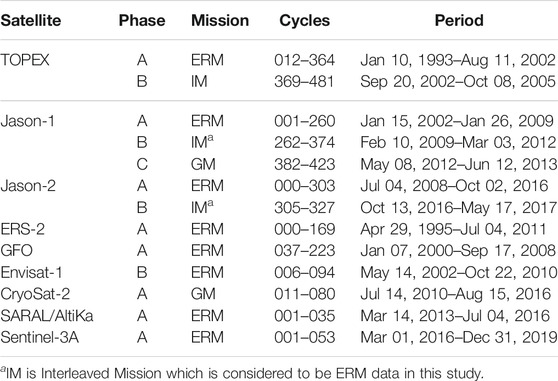
TABLE 1. Summary of all altimetry data for MSS computation.
All satellite altimetry data obtained in this study are provided by the Technical University of Delft, Netherlands. They are accessible via the RADS server in UTM, thus yielding the latest information on orbits and geophysical corrections. Furthermore, the acquired data are preprocessed based on the best range and geophysical corrections in the context of the Malaysian region. This includes rendering and removing invalid data as well as generating the corresponding refined geophysical corrections. Most of the range and geophysical corrections applied for this model are underpinned and guided by user manuals and progressive experiences from previous studies (Scharroo et al., 2013; Din et al., 2014; Yahaya et al., 2016; Hamid et al., 2018; Din et al., 2019; Zulkifle et al., 2019). Supplementary Table S1 differentiates a list of range and geophysical corrections implemented by Yahaya et al. (2016), Zulkifle et al. (2019), and UTM20 MSS. Most geophysical corrections and models applied are similar to previous regional models except for load and ocean tides. The results of ocean tide are rectified by the GOT4.10c ocean tide model for all altimetry missions (Ray, 2013).
Altimetry Data Processing Method
In most cases, the MSS model is typically determined via a temporal average method. It depends on the following processes: data selection and preprocessing, ERM mean track derivation from collinear analysis, removal of GM sea level variability, crossover minimization, and data gridding. After applying geophysical correction and removing the bias in the preprocessing section, the following action is to remove the sea level variability of ERM and GM data. Figure 1 illustrates the general processing flow in establishing the MSS model.
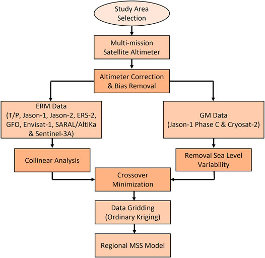
FIGURE 1. Overall data processing flows in computing MSS model.
Eliminating the Sea Level Variability of ERM and GM Data
The collinear analysis is the method of correcting MSS gradients by taking into account along-track gradients (Braun et al., 2004). The purpose of collinear analysis of ERM data is to eliminate the sea level variability, consisting of seasonal and inter-annual signals. It also strives to achieve average along-track SSH data. The average track is calculated from the selected track and corresponding collinear track. In this study, the collinear track of first cycle observations is designated to be the reference track. Subsequently, collinear analysis computes each SSH point of collinear tracks similar to the reference track (Jiang et al., 2002; Jin et al., 2016; Yuan et al., 2020).
The collinear analysis in this study is used to measure average along-track SSH. Necessary steps are taken in the process of calculating the average along-track SSH. The first is data filtering, in which the data will be discarded when the difference between SSH and MSS is greater than 1 m, and the new MSS will be re-calculated. Moving average technique is implemented to eliminate the annual and semi-annual variations in this study. The formula of the moving average technique is expressed as in Equation 2 (Smith, 2003).
where
The impact of SSH time variation for ERM can be reduced by subjecting it to time-averaging. However, unlike ERM data, SSH observations in the GM of satellite altimetry must be handled differently to minimize time variation. Time-averaging is only attributable to the GM data that not having the typical feature of the repeated period; thus, it is not suitable for the GM satellite tracks. Two methods can be implemented to remove the sea level variability from GM satellite data. The first method applies the correction based on seasonal variations fitting from the gridded sea level variation time series introduced by Andersen et al. (2006) and Andersen and Knudsen (2009). This method describes the seasonal variations are extracted using the gridded sea level variation time series, interpolated to the GM observations, and adjusted. The bias, linear trend, seasonal, and annual signals of sea level variations at each gridded point are fitted using a polynomial function. The second method is based on the interpolation of sea level anomalies (SLA) introduced by Schaeffer et al. (2012) and Jin et al. (2016). In this method, the sea level variability of GM data can be adjusted by the sea level variability of ERM data which hold as a reference at the spatial and temporal positions of GM data. Schaeffer et al. (2012) stated that the optimal analysis could be used to interpolate the SLA of one or more missions considered as a reference at the spatial and temporal position that would be adjusted for ocean variability. According to Jin et al. (2016), the correction based on the SLA interpolation showed remarkable improvement in removing the sea level variability.
Therefore, the method implemented in this study is based on the interpolation of SLA. The delayed-time Developing Use of Altimetry for Climate Studies (DUACS) Level 4 gridded SLA maps (Dibarboure et al., 2012) are used as a reference at spatial and temporal positions of the GM data. This model is obtained from the European Copernicus Marine Environment Monitoring Service (CMEMS) via https://resources.marine.copernicus.eu/. The corresponding hourly gridded SLA time series are computed to adjust the GM data listed in Table 1 (i.e., Jason-1 Phase C, and CryoSat-2). The sea level variability of Jason-1 Phase C, and CryoSat-2 can be adjusted by the DUACS hourly gridded SLA time series to their observation duration as shown in Table 2.

TABLE 2. DUACS corresponding data used for reduction of GM sea level variability data.
Determination of the UTM20 Mean Sea Surface
After removing the sea level variability from ERM and GM data, it is expected that the seasonal sea level variations can be immensely eradicated. Besides, the part of radial orbit error is also expected to be reduced through the orbit calculation of ERM and GM data, adequately handled by RADS. Nevertheless, some errors such as residual orbit error and residual geophysical corrections are still present in the measurements. Thus, crossover adjustment is performed to reduce these errors. Crossover adjustment is performed due to orbital errors and inconsistencies in the satellite’s orbit frame (Din et al., 2019). The crossover minimization is based on the discrepancy between two intersecting points for integrating multi-satellite altimetry data or the correction of measurements. The radial orbit error is one of the predominant factors affecting the altimetry data in the classical crossover adjustment. This error will be accurately modeled by either time-dependent or distance-dependent polynomial (Wagner, 1985; Rummel, 1993). According to Hamid et al. (2018), it is a practical approach geared towards reduced orbit errors and improved multi-mission satellite altimetry measurements. Besides, it can minimize the crossover between ascending and descending height differences and concurrently limit the track errors. Since the average along-track SSH of the T/P series is used as a reference in this study, each satellite including ERS series and CryoSat-2 are calibrated to the T/P reference.
An interpolation technique is performed to create the MSS model grid after applying crossover adjustment. Based on the previous regional MSS model, both models developed by Yahaya et al. (2016) and Zulkifle et al. (2019) applied the inverse distance weighting (IDW) technique for MSS data gridding. Although Jin et al. (2016) and Yuan et al. (2020) stated that the least square collocation (LSC) is the most suitable method for gridding, this study implements ordinary kriging for the regional UTM20 MSS model. The kriging method is similar to IDW, in which it weights the surrounding measured values to compute a prediction at predicted points. The formula is expressed in Equation 3 (Environmental Systems Research Institute, 2016a).
where
The ordinary kriging in this study use covariance function instead of semivariogram to express autocorrelation. The covariance functions quantify the assumption that the nearby measurements appear to be equal to those farther apart. It measures the strength of statistical correlation as a function of distance. The covariance function modeling method fits the covariance curve to the empirical data, in which the aim is to obtain the best fit model. Later, this model is utilized in the predictions. The covariance function of the ordinary kriging method is expressed in Equation 4 (Environmental Systems Research Institute, 2016b).
where
Moving Average Technique of 19-years Interval
The moving average technique of 19-year intervals has been introduced by Yuan et al. (2020). The result showed that this technique had effectively increased the precision of the MSS model. Consequently, the moving average of the 19-year technique is also applied for the computation of the UTM20 MSS model. The satellite altimetry data from 1993 to 2019 are classified into eight groups as listed in Supplementary Table S2, where each group has a 19-year interval data span.
The satellite altimetry data from each group is used separately to compute the MSS model with a 1.5-min by 1.5-min grid over Malaysian seas. Thus, eight MSS models are obtained from each group. Last, the grid of eight MSS models is averaged at each grid point to obtain UTM20(G) MSS. The averaging step is expressed in Equation 5.
where
Computation of the UTM20 Mean Dynamic Topography
The practical approach renders the process of MDT quantified from MSS and geoid model to be conceptually straightforward. In general, MDT
where
The UTM20 MSS is in the mean tide system, while the permanent tide system of MyGeoid_2017 is unclear. Based on Keysers et al. (2015), geoid undulations may be used in any system. However, EGMs are generally issued as both in the tide-free and zero tides. In general, most regional geoids acquired their tidal system from the EGM, but the system should be precisely specified. Thus, it is expected that MyGeoid_2017 is in tide-free system. Both models must be in the same permanent tide system in order to compute MDT precisely. Here, UTM20 MSS is converted to tide-free system by using the conversion formula (in cm) as expressed in Equation 7 (Ekman, 1989; Keysers et al., 2015).
where
Spatial averaging filtering methods are likely to be more reliable and precise for regional MDT applications than spectral filtering methods (Losch et al., 2007; Knudsen and Andersen, 2013). Spatial filters with a Gaussian-like roll-off have more accurate results than those with sharp space cut-offs. 2D isotropic Gaussian function is expressed as Equation 8 (Fisher et al., 2003).
where x is the distance from the origin in the horizontal axis, y is the distance from the origin in the vertical axis, and σ is the standard deviation of the distribution, which is also defined as the filter radius. Hence, the unfiltered regional MDT is computed by differentiating the UTM20 MSS model and a local precise gravimetric geoid, MyGeoid_2017. A spatial filter is applied to smooth the unfiltered MDT. The spatial filter is an average filter at which the kernel is
Results
Temporal Sea Level Variability Correction
The ERM data of satellite altimetry used in this study, as listed in Table 1, undergo collinear analysis to eliminate seasonal variations and to obtain the average along-track SSH within the observation period. Since the GM data of satellite altimetry are involved in the MSS model, the corrections of sea level variability of the data as listed in Table 1 are principally considered. Only two satellite missions from GM data are involved in establishing the UTM20 MSS model, namely, Jason-1 Phase C and CryoSat-2. The statistical results of crossover differences before and after the removal of seasonal variations of ERM and GM data are listed in Table 3. T/P series Phase A shows the highest accuracy among others, which is within 4 cm. In addition, other ERM data show significant improvement of SSH accuracy, which is better than 10 cm. It can be deduced that the impact of seasonal variations on SSH via collinear analysis has been minimized. Apart from that, the precision of ERM SSH data is considerably better than 10 cm. For GM data, the results inferred that the precision of both GM data is significantly improved after applying the correction. The crossover differences are improved within 6–7 cm.
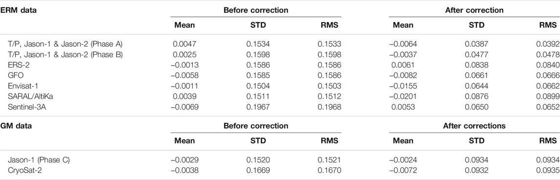
TABLE 3. Statistical results of crossover difference before and after seasonal correction (units are in meters).
Supplementary Figure S2 shows that the seasonal variations from ERM data are eliminated significantly. In the spatial domain of the SSH time series, the RMS of SSH before seasonal correction is 9.95 cm. After detrending the data and removing the seasonal signal, the RMS of SSH is significantly improved to 2.01 cm. The removal of seasonal variation is further analyzed by comparing the signal in the spectral domain. It signifies that after applying seasonal correction, the power spectrum of SSH frequency is lower than the signal before applying the seasonal correction.
Supplementary Figure S3 shows the achievement in correcting the seasonal variations of Jason-1 Phase C GM data. The upper map illustrates the height differences between SSH of Jason-1 Phase C GM and UTM20 MSS, where the sea level variability is induced in the measurements (Supplementary Figure S3A). It clearly indicates that this discrepancy is mainly prevailed by sea level variability. Supplementary Figure S3B shows the height differences between Jason-1 Phase C GM SSH and UTM20 MSS, where the sea level variability of GM data is removed. The RMS of Jason-1 Phase C GM data is remarkably improved from 10.27 to 6.53 cm. Therefore, it can be concluded that the sea level variability of ERM and GM data have been processed appropriately prior to computing the regional MSS model.
UTM20 Mean Sea Surface Model
After correcting the sea level variability of ERM and GM data, crossover minimization is performed to reduce the existing errors as mentioned in Determination of the UTM20 Mean Sea Surface section. Since T/P series Phase A has the highest orbit accuracy among others, it is used as the foundation for adjustment. Thus, each of the missions is adjusted towards the foundation. Table 4 shows the statistical results before and after crossover minimization. The results show that the accuracy of crossover difference is essentially improved after crossover minimization is performed. All missions’ accuracy is below 10 cm after applying crossover minimization.
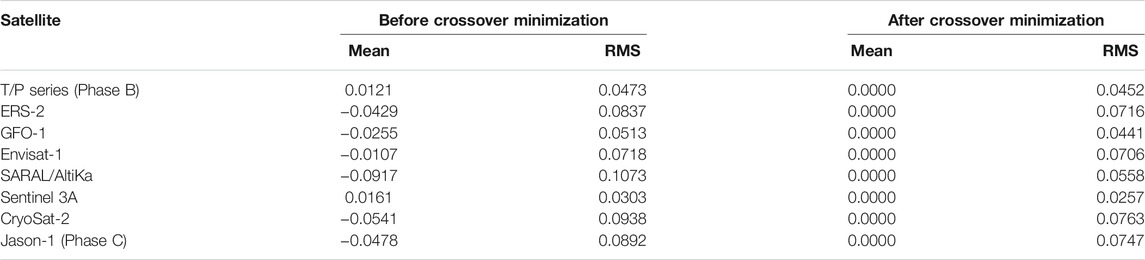
TABLE 4. Statistical results of crossover differences before and after crossover minimization (units are in meters).
A regional MSS model is successfully generated by adopting an ordinary kriging interpolation method. Two types of UTM20 MSS models are established in this study. The first model is established using the moving average technique of 19-year interval where MSS from each of the eight satellite altimetry groups is interpolated from the common average approach to form eight gridded MSS models. The average of these eight gridded MSS models is then computed to obtain UTM20(G) MSS model. The second model, namely, UTM20(F) MSS model, is established without adopting a 19-year moving average technique but by interpolating multi-mission satellite altimetry data as listed in Table 1 from a standard average method. Since Yuan et al. (2020) have conducted the study on a 19-year moving average technique and the results showed that the model’s accuracy had improved significantly; this technique is once again verified in this study within the region of the Malaysian seas. It is crucial to determine whether the moving average of the 19-year technique can significantly increase the accuracy of the regional MSS model as the study area is induced by significant tidal errors in altimetry measurements.
Figure 2 illustrates the UTM20(G) MSS model where the height of MSS increases gradually from Malacca Straits towards the Sulu Sea. All four regions of Malaysian seas incorporated in this study yield different MSS values based on the WGS84 reference ellipsoid. In particular, the Malacca Straits has the lowest MSS, which is located below the reference ellipsoid, while Celebes Sea generated the highest MSS value. It should be noted that the MSS height at the Celebes Sea and the Sulu Sea are higher than the South China Sea and Malacca Straits. Henceforth, this regional MSS model is proven essential for charting datum, observing sea-level changes and concurrently encouraging geophysical and oceanographic applications such as tidal prediction and sea-level rise study.
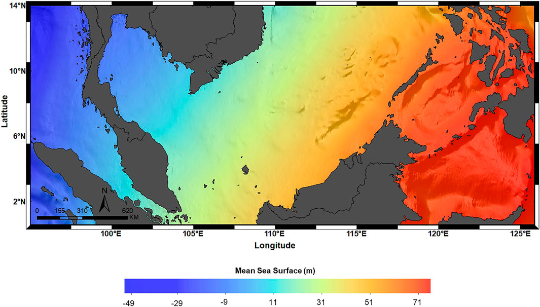
FIGURE 2. UTM20(G) MSS model developed by using a 19-year moving average technique.
UTM20 Mean Dynamic Topography Model
Different MDT models utilize various geoid models in the computation of MDT, rendering it crucial to select the best geoid model. For this research, MyGeoid_2017 is adopted to be subtracted with the UTM20 MSS model to compute the regional UTM20 MDT model. It is selected due to MyGeoid_2017, a local precise gravimetric geoid model developed by the government agency, DSMM, which is often utilized by the local surveyor community as a locally based geoid separation model for the establishment of vertical positioning aspects in surveying and work practices. The geodetic MDT is calculated using a pointwise gridded approach between the gridded MSS model and geoid height as expressed in Equation 6. Figure 3A shows the preliminary UTM20 MDT using the pointwise approach. The figure shows that the local geoid omission errors leak into the MDT due to the small scale of MSS missing from the geoid. This means that the detail is obscured by noise (gross features) due to geoid omission errors.
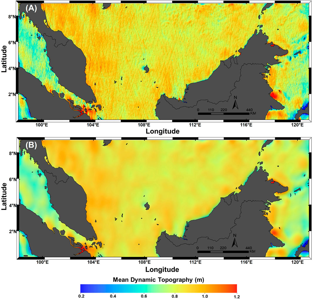
FIGURE 3. UTM20 Mean Dynamic Topography model. (A) Preliminary (unfiltered) model. (B) Final (filtered) model.
Bingham et al. (2008) stated that the problem of geoid omission error contaminated the MDT could be simply overwhelmed by using the spatial averaging filter to smooth the MDT. For instance, Jayne (2006) had conducted a Hamming window for spatial filtering. However, this study is utilizing a Gaussian-like roll-off filter to smooth the final regional UTM20 MDT. With few experiments, six sigma, which is approximately 70 km Gaussian filter size, is carried out to remove the scale of the short-wavelength noise and preserve mesoscale features in the study area. Not only that, but filtering can also eliminate the ground track striation, so-called the orange skin effect. Figure 3B shows the final UTM20 MDT computed after applying the spatial averaging Gaussian filter.
Thus, it can be concluded that the filtered regional MDT in this study preserves the spectral content with the shortest wavelength of approximately 70 km. The MDT has the highest value near the Gulf of Thailand, as shown in Figure 3. The pattern shows that the slope of MDT decreases from the Gulf of Thailand towards the south of Peninsular Malaysia. However, the pattern of the MDT slope decreases as it goes toward the northwest of the Malacca Straits. It can also be deduced that the South China Sea has the highest MDT values compared to the Malacca Straits, the Celebes Sea, and the Sulu Sea. Meanwhile, the Malacca Straits has the lowest MDT values among others.
Discussion
This section mainly discusses the verification of the regional UTM20 MSS model and UTM20 MDT model. In general, assessing the accuracy of the MSS model developed from satellite altimetry is a very challenging process. This is due to the high accuracy of SSH determination provided by the satellite altimeter and almost all satellite altimetry data are implemented in the derivation of the MSS model. Therefore, the reliability and accuracy of the UTM20 MSS model are verified by comparing the model with two global MSS models, namely, DTU18 and CLS15 MSS. For UTM20 MDT, the model is verified with two global MDT models, namely, DTU15 and CLS18 MDT. The accuracy of both regional MSS and MDT models are also verified with Global Navigation Satellite System (GNSS) leveled tide gauges along the coast of Peninsular Malaysia.
Verification of the UTM20 MSS with the global MSS models
The discrepancy between MSS models relies on the satellite altimetry data involved in computation and processing techniques (Schaeffer et al., 2012; Yuan et al., 2020). The satellite mission of Sentinel-3A is not included in CLS15 and DTU18 models, whereas it is included in UTM20(G) and UTM20 (F). Likewise, the SARAL/AltiKa mission is involved in DTU18, UTM20(G), and UTM20(F), but not in the CLS15 model. Moreover, the regional MSS models have distinct reference periods compared to the global MSS models. The reference period for UTM20(G) and UTM20(F) spans from 1993 to 2019. Meanwhile, the reference period for CLS15 and DTU18 spans from 1993 to 2012. The data processing method also can cause the discrepancy between MSS models. This includes the pre-processing data that involve the application of range and geophysical corrections, the treatments in removing sea level variability, and the utilization of data interpolation method.
DTU18, CLS15, UTM20(G), and UTM20(F) are compared in terms of gridded MSS points as listed in Tables 5, 6. Table 5 shows the statistical result of the comparison for all points. Meanwhile, Table 6 shows the statistical comparison results for the points where the outliers in the difference are excluded by three times of standard deviation (3σ). The exclusion would prevent contamination by wrong observations around the coastal regions and islands. Both tables show that the standard deviation (denoted as STD) values for the comparison of UTM20(G) and UTM20(F) with CLS15 are lower than the comparison with DTU18. This implies that there are distinct differences between regional models and DTU18, and the best consistency is shown by the UTM20(G), UTM20(F), and CLS15 models. A total of 3,915 points have been rejected after applying three sigmas of the difference, and it shows a significant improvement of accuracy in MSS models. The distribution of rejected points is illustrated in Supplementary Figure S4. It clearly indicates that most of the rejected points are distributed nearshore regions. This is due to the contamination within the altimetry footprint when approaching the land, causing inaccurate observation.
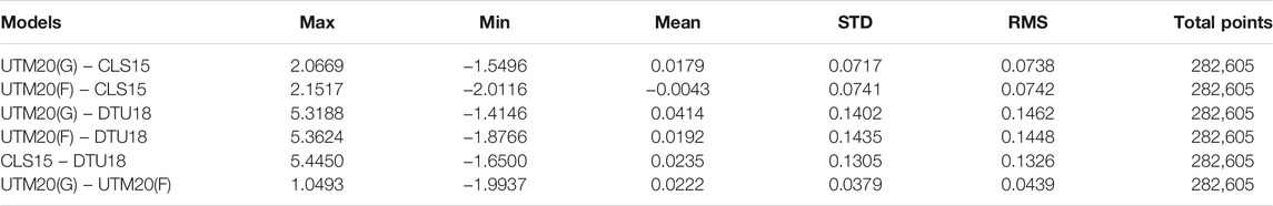
TABLE 5. Statistical results of the comparison between four MSS models (all points are included) (units are in meters).

TABLE 6. Statistical results of the comparison between four MSS models (exclusion data by 3σ) (units are in meters).
These four MSS models are further verified in the offshore and coastal regions (20 km from the land). The statistical results of the differences are tabulated in Supplementary Table S3. All points are involved in the computation of statistical results. UTM20(F), UTM20(G), CLS15, and DTU18 are denoted as U(F), U(G), CLS, and DTU, respectively. The results show that the STDs of U(G)-DTU, U(F)-DTU, and CLS-DTU are less than 5 cm in the offshore region. However, these STDs are more prominent in the coastal region, which is within 30–33 cm. Significant differences exist between the models because of the contrasting satellite altimetry data and preprocessing techniques being executed. The STD of differences between UTM20(F) and UTM20(G) is 2.4 and 7.4 cm in the offshore and coastal regions, respectively. Moreover, UTM20(G) is remarkably more accurate than UTM20(F). This is proven where the STD of comparison between CLS15 and DTU18 models with the UTM20(F) is higher than the STD of comparison between those two models with UTM20(G). Therefore, the UTM20(G) MSS model is selected as the final regional UTM20 MSS model and further utilized for MDT computation.
The accuracy of regional MSS models developed by UTM is compared and tabulated in Table 7. The first model was developed by Yahaya et al. (2016) (denoted as MSS1) and then further enhanced by Muhammad (2018) and Zulkifle et al. (2019) (denoted as MSS2). Although the methodology on the computation of both MSS models is unclear, these previous regional models have computed the statistical results by comparing them with the DTU model. Thus, the root mean square error (RMSE) between previous models and DTU are compared with RMSE between UTM20 MSS and DTU model. The result shows significant improvement in accuracy for the models from 2 to 0.14 m misfit errors. This indicates that the UTM20 MSS model successfully scrutinizes the proper mean derived from along-track SSH and properly removed sea level variability and other errors in the data processing.
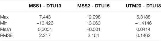
TABLE 7. Comparison of RMS misfit between regional MSS model and DTU models in Malaysian seas (units are in meters).
Verification of the UTM20 MSS With GNSS Leveled Tide Gauge
Further verification of MSS is conducted by comparing the UTM20 MSS with mean sea level (MSL) derived from in-situ GNSS leveled tide gauges. Eleven tide gauge stations around Peninsular Malaysia are selected for the purpose of verification. The MSL at the respective tide gauges is derived from 23 years observation period covering from 1993 to 2015 by a simple averaging method. As all tide gauge benchmarks (TGBMs) are referenced to zero tide gauge, the Tide Gauge GNSS Campaign 2019 was performed to shift the tidal measurement relative to the reference ellipsoid. The campaign was not implemented in Sabah and Sarawak-based tide gauge stations due to the lack of logistics requirements and time constraints for mobilization and demobilization in the two states. Supplementary Figure S5 illustrates eleven DSMM tide gauge stations involved in the Tide Gauge GNSS Campaign 2019 and the relationship of various vertical surfaces towards achieving the tidal measurement with respect to the ellipsoidal surface (Azhari, 2003). The formula to obtain the MSL with respect to ellipsoid is shown in Equation 9.
where
UTM20 MSS, CLS15 MSS, and DTU18 MSS models are extrapolated to the tide gauges location using bilinear interpolation. This interpolation method uses a distance-weighted average of the four nearest point values to estimate a new point value. These MSS models at extrapolated points are compared with MSL derived from GNSS leveled tide gauges. Table 8 shows the statistical results of differences between MSL of GNSS leveled tide gauges and MSS of satellite altimetry models at extrapolated points. The results show that the mean height differences between tide gauges MSL and UTM20 MSS are −7.8 cm with a standard deviation of 7.5 cm. The accuracy of UTM20 and CLS15 at tide gauges location is almost similar, which is within 7 cm, while the accuracy of DTU18 is greater than both models, which is 10 cm. In addition, the height differences between the MSS models and GNSS leveled tide gauges ranging from −25 to 11 cm. This might be due to a decrease in the accuracy of altimetry observations when assessed closer to the coast. No available altimetry data or invalid value of MSS might be obtained in this study as the altimetric measurements approach within 5–10 km to the coast. According to Vignudelli et al. (2019), the altimetry sensors were not highly sufficient for the coastal region to reach precise sea levels due to the corrupted waveforms. This might also be due to a few forcing factors affecting the sea level changes in coastal areas. For instance, the SSH derived from satellite altimetry includes contributions from ocean thermal expansion and ocean circulation, water movement from land to ocean, and changes in land water storage. The larger-scale changes are covered by the sea level fluctuations from tides and coastal processes due to air pressure effects and wind setup (Woodworth et al., 2019). This resulted in the proposal to implement high-resolution coastal altimetry data and multiple retracking methods to improve SSH estimation in the coastal areas (Idris et al., 2017; How et al., 2020).
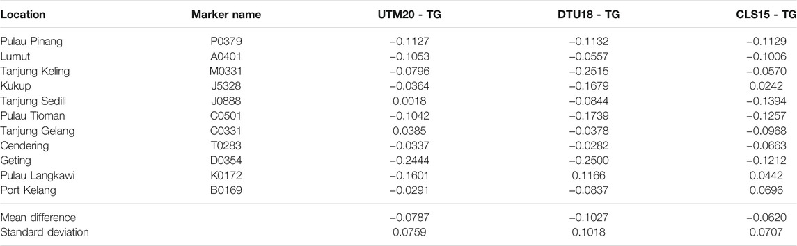
TABLE 8. Statistical result of differences between tide gauges MSL and extrapolated points of satellite altimetry MSS (units are in meters).
Verification of the UTM20 MDT With the Global MDT Models
Each MDT model is provided with a particular spatial resolution and time coverage. Nevertheless, a similar MDTs’ characteristic is needed for consistent comparison. In this study, CLS18 MDT and DTU15 MDT are utilized for comparison with UTM20 MDT. All the models are resampled with a spatial resolution of 2-min by 2-min. The problem that arises in comparing MDT models is that each model is computed with respect to different reference surfaces, which occurred on three of the models used in this study. UTM20 MDT is computed by subtracting the UTM20 MSS with local gravimetric geoid (MyGeoid_2017). Meanwhile, DTU15 MDT is developed by subtracting the DTU15 MSS with the EIGEN-6C4 geoid model (Andersen et al., 2015), and CLS18 MDT is computed by differentiating the CLS15 MSS with the GOCO5S geoid model (Mulet et al., 2019). Finalizing Surveys For the Baltic Motorways Of The Sea FAMOS (2017) proposed that a comparison of MDT anomalies be performed to overcome this problem. It is computed by de-meaning the values for each surface. This method is simply comparing the variability of each MDT rather than its magnitude. Figures 4A–C show the MDT anomalies of three MDT models, which are CLS18, DTU15, and UTM20, respectively. The figures clearly indicate that all the models have a similar pattern, although UTM20 MDT anomalies show an unsmooth surface compared to CLS18 and DTU15, which might be due to the models’ resolutions. The dark blue color that appeared at the south of Celebes Sea and the south-west Sumatra in UTM20 MDT anomalies is due to the data being near the edge of the studied area (Figure 4C). Therefore, smoothing and averaging techniques are inappropriate in such edge.
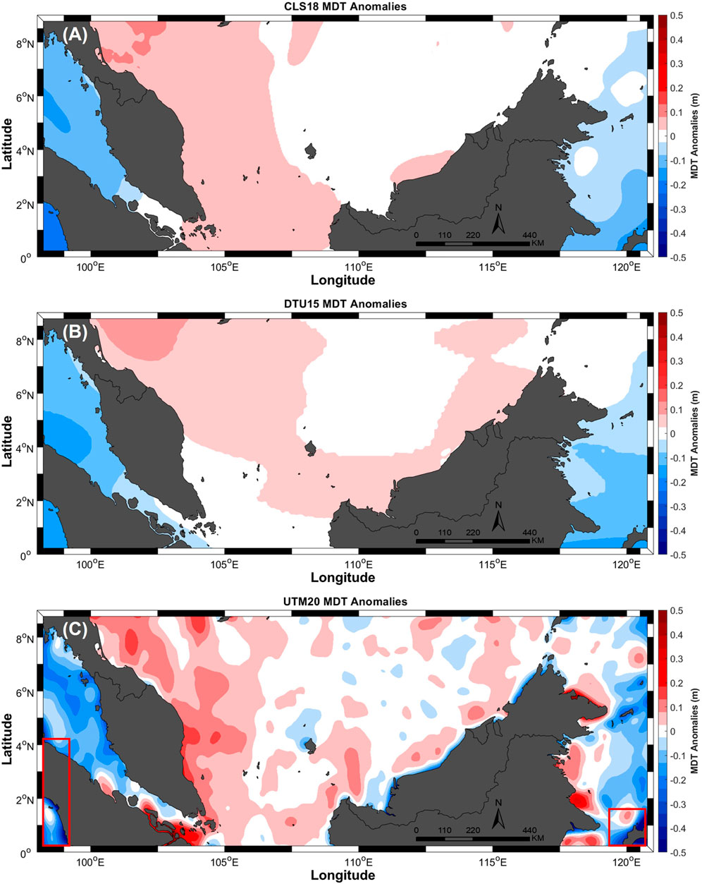
FIGURE 4. MDT anomalies of three models: (A) CLS18 model; (B) DTU15 model; (C) UTM20 model.
The statistical results of the MDT anomalies differences are compared as shown in Table 9. MDT anomalies between CLS18 and DT15 show the lowest STD of the differences, which is 1.67 cm. Meanwhile, MDT anomalies between UTM20 and DTU15 show the highest STD of the differences, which is 5.5 cm. MDT anomalies between UTM20 and CLS18 have STD of 5.1 cm. Thus, it can be inferred that MDT anomalies of UTM20 have better agreement with CLS18. The discrepancy between models may be due to the differences in the epoch at which the models are estimated.
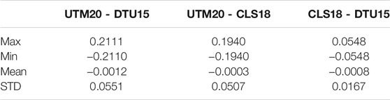
TABLE 9. Statistical results of the MDT anomalies differences (units are in meters).
Verification of the UTM20 MDT With Tide Gauges Geodetic MDT
Although evaluating the discrepancies of MDT anomalies between regional and global models provides an opportunity for comparison, it does not clearly indicate the approximate accuracy of the model. Further verification is needed to estimate the reliability of UTM20 MDT. The efficiency of the MDT models is analyzed by comparing them with in-situ data from the DSMM tide gauge stations. The precise local geoid model (MyGeoid_2017) is utilized for the MDT computation at tide gauges (denoted as MDTTGBM) to ensure its consistency with the computed MDT models. Also, the tide system of all measurements is set to be identical to the tide-free system. Note that no filtering is performed in the computation of MDT at tide gauge stations. The MDT models of UTM20, CLS18, and DTU15 are extrapolated to the tide gauge stations using the bilinear interpolation method. In order to simplify the comparison, the MDT values at Pulau Langkawi are arbitrarily fixed to zero. Apart from that, all MDT values at other tide gauge stations are adjusted to Pulau Langkawi.
Figure 5A depicts the comparison of the MDT models with the MDTTGBM. The range of the entire MDT along the coast of Peninsular Malaysia is within 0–0.4 m, which is higher along the east coast and lower in the west coast region (refer to Figure 4). Also, Figure 5B shows the absolute differences between the MDT models with respect to MDTTGBM. The absolute differences between UTM20 MDT and MDTTGBM are lower in most tide gauge stations, which display below 0.15 m compared to the CLS18 and DTU15 MDT. The highest MDT differences between UTM20 MDT and MDTTGBM among all tide gauge stations are within 0.12 m, while CLS18 and DTU15 record 0.25 and 0.27 m, respectively. This figure clearly indicates that the effects of low accuracy of SSH observations from altimetry in the coastal area and interpolation method used may translate the actual shifted values.
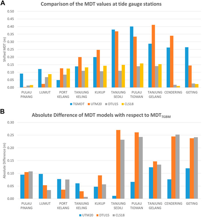
FIGURE 5. (A) Comparison of the MDTTGBM values with MDT models (UTM20, CLS18, and DTU15) at tide gauge stations. (B) The absolute difference of the MDT models with respect to the MDTTGBM at which MDT at Pulau Langkawi is fixed to zero in all models and others are adjusted accordingly.
The statistical results of the absolute differences between MDT models and MDTTGBM are also computed and tabulated in Table 10. The UTM20 MDT has the smallest STD of 3.80 cm compared to the CLS18 MDT and DTU18 MDT, where the STD differences are 9.55 and 9.80 cm, respectively. Note that the value of MDT differences at each tide gauge station in Table 10 is shifted to Pulau Langkawi tide gauge station. Therefore, considering the results of all tide gauge stations, it can be concluded that UTM20 MDT has a better statistical agreement with independent geodetic tide gauge MDT (MDTTGBM) compared to CLS18 MDT and DTU15 MDT.
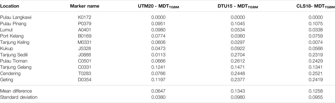
TABLE 10. Statistical results of the MDT models (UTM20, CLS18, and DTU15) with respect to the tide gauge MDT (MDTTGBM) (units are in meters).
Conclusion
This article conclusively described the new regional UTM20 MSS and UTM20 MDT models as well as the manner in which they are established. In particular, the UTM20 MSS entailed the altimetry-averaged height of the SSH, which derived from an integration of nine satellites encompassing the period from 1993 to 2019. Two types of regional UTM20 MSS models are established, namely, UTM20(G) and UTM20(F). UTM20(G) is established by applying a 19-year moving average technique, while UTM20(F) is established using a conventional average method. Both models are compared with CLS15 MSS and DTU18 MSS in the Malaysian seas. The results show that all of the established models in this study are at par with the reference models. Apart from that, the UTM20(G) shows higher accuracy than UTM20(F), thus, indicates that the moving average technique of a 19-year interval significantly improved the accuracy of the MSS model in Malaysian seas. Consequently, the UTM20(G) has been chosen to be the final regional MSS model in this study. Carried out on a 1.5-min by 1.5-min grid, it depicted an improvement compared to the previous regional UTM MSS models by successfully measuring the proper mean derived from the along-track SSH. This has been reflected in the misfit value of 14.6 cm between UTM20 MSS and the DTU model compared to the previous model’s misfit value of 2-m. Moreover, UTM20 MSS has been validated by comparing it with the MSL from GNSS leveled tide gauges, yielding the accuracy of MSS within 7 cm at all stations.
Furthermore, UTM20 MDT has been established by differentiating the local precise gravimetric geoid (MyGeoid_2017) with the UTM20 MSS model. After subtracting the MSS with the local geoid, the derived MDT undergoes Gaussian spatial filtering to smooth the unwanted noise signal. UTM20 MDT is then compared with the CLS18 MDT and DTU15 MDT models, and it is also compared with 11 tide gauges derived geodetic MDT for statistical data assessment. The findings show that UTM20 MDT is in solid agreement with global models, despite the different epoch of MSS used in each model. The verification results of MDT at tide gauge stations disclosed that the UTM20 MDT has the lowest standard deviation of MDT discrepancies, which is 3.80 cm compared to the CLS18 MDT (9.55 cm) and DTU15 MDT (9.80 cm).
In line with MSS being an essential reference for sea level variability, the UTM20 MSS model indicates relatively better accuracy than previous models. However, specific processes have not been performed in the coastal areas, which, in turn, will become the critical elements for future improvements in deriving MSS and MDT models. For instance, adopting recent radar technology such as Synthetic Aperture Radar (SAR) mode on CryoSat-2 and Sentinel-3A as well as operating high along-track sampling of SARAL/AltiKa (Ka-band altimetry) is essential to enhance the quality of the models near the coast. Indeed, the retracking of altimetry waveforms can increase the accuracy of SSH in the coastal region. Thus, attempting the retracking process for the altimetry ranges is recommended, as it is a task that may potentially enhance the process of MSS and MDT in the future.
Data Availability Statement
The original contributions presented in the study are included in the article/Supplementary Material; further inquiries can be directed to the corresponding author.
Author Contributions
AD and DW provided the initial ideas and designed the experiments for this research. MH performed the designed experiments. MH and MP analyzed the outcome data. MH wrote the manuscript with contributions from AM, DW, and MY. All authors were involved in discussions throughout the development.
Funding
This project is funded by the Ministry of Higher Education (MOHE) under the Fundamental Research Grant Scheme (FRGS) Fund, Reference Code: FRGS/1/2020/WAB05/UTM/02/1 (UTM Vote Number: R.J130000.7852.5F374).
Conflict of Interest
The authors declare that the research was conducted in the absence of any commercial or financial relationships that could be construed as a potential conflict of interest.
Publisher’s Note
All claims expressed in this article are solely those of the authors and do not necessarily represent those of their affiliated organizations, or those of the publisher, the editors and the reviewers. Any product that may be evaluated in this article, or claim that may be made by its manufacturer, is not guaranteed or endorsed by the publisher.
Acknowledgments
The authors would like to express their sincere appreciation to the TU Delft, NOAA, Altimetrics LLC for providing the altimetry data through RADS server, AVISO+ through the Centre National d’Etudes Spatiales (CNES) for providing the CLS15 MSS and CLS18 MDT, the Space Research Centre of the Technical University of Denmark (DTU) for providing DTU18 MSS and DTU15 MDT, and Copernicus Marine Environment Monitoring Service (CMEMS) for providing the DUACS L4 gridded SLA. Special thanks to the Department of Surveying and Mapping Malaysia (DSMM) for kindly contributing the local precise geoid model and tidal data for this study.
Supplementary Material
The Supplementary Material for this article can be found online at: https://www.frontiersin.org/articles/10.3389/feart.2021.665876/full#supplementary-material
References
Andersen, O. B., and Knudsen, P. (2009). DNSC08 Mean Sea Surface and Mean Dynamic Topography Models. J. Geophys. Res. 114 (11), 327–432. doi:10.1029/2008JC005179
Andersen, O. B., Knudsen, P., and Stenseng, L. (2018). A New DTU18 MSS Mean Sea Surface – Improvement from SAR Altimetry. 172.” in Abstract from 25 years of progress in radar altimetry symposium, September 24–29, 2018. Portugal; Ponta Delgada. Available at: https://backend.orbit.dtu.dk/ws/files/163304443/25YPRA_Abstract_Book.pdf (Accessed October 20, 2020).
Andersen, O. B., Piccioni, G., Stenseng, L., and Knudsen, P. (2015). The DTU15 Mean Sea Surface and Mean Dynamic Topography-Focusing on Arctic Issues and Development.” in Oral Presentation, in the 2015 OSTST Meeting, Virginia, USA. Editors P. Bonnefond, J. Willis, and Reston Available at: https://meetings.aviso.altimetry.fr/fileadmin/user_upload/tx_ausyclsseminar/files/OSTST2015/GEO-03-Andersen_MSSH_OSTST.pdf (Accessed October 29, 2020).
Andersen, O. B., Piccioni, G., Stenseng, L., and Knudsen, P. (2016). The DTU15 MSS (Mean Sea Surface) and DTU15LAT (Lowest Astronomical Tide) Reference Surface.” in Proceedings of the ESA Living Planet Symposium 2016, May 9–13, 2016. Prague, Czech Republik. Editors L. Ouwehand Prague, J. Willis, and Reston. Available at: https://ftp.space.dtu.dk/pub/DTU15/DOCUMENTS/MSS/DTU15MSSþLAT.pdf (Accessed April 18, 2020).
Andersen, O. B., and Scharroo, R. (2011). Range and Geophysical Corrections in Coastal Regions: And Implications for Mean Sea Surface Determination. Coastal altimetry, 103–145. doi:10.1007/978-3-642-12796-0_5
Andersen, O. B., Vest, A. L., and Knudsen, P. (2006). The KMS04 Multi-mission Mean Sea Surface.” in Proceedings of the Workshop GOCINA: Improving Modelling of Ocean Transport and Climate Prediction in the North Atlantic Region Using GOCE Gravimetry. Novotel, Luxembourg. Editors P. Knudsen 25, 103–106. Available at: http://gocinascience.spacecenter.dk/publications/4_1_kmss04-lux.pdf (Accessed May 15, 2020).
Astina, T. (2017). Bathymetry Mapping over Malaysian Seas Using Satellite Geodetic Missions. Skudai: MSc Thesis. Universiti Teknologi Malaysia.
Azhari, B. M. (2003). An Investigation of the Vertical Control Network of Peninsular Malaysia Using a Combination of Levelling, Gravity, GPS and Tidal DataPhD Thesis. Skudai: Universiti Teknologi Malaysia.
Bingham, R. J., Haines, K., and Hughes, C. W. (2008). Calculating the Ocean's Mean Dynamic Topography from a Mean Sea Surface and a Geoid. J. Atmos. Oceanic Tech. 25 (10), 1808–1822. doi:10.1175/2008JTECHO568.1
Braun, A., Yi, Y., and Shum, C. K. (2004). Altimeter Collinear Analysis. Satellite Altimetry and Gravimetry: Theory and Applications. Lecture Notes. Available at: https://geodesy.geology.ohio-state.edu/course/gs873.2013/lectures/alt_collinear_analysis.pdf (Accessed October 29, 2020).
Dibarboure, G., Renaudie, C., Pujol, M.-I., Labroue, S., and Picot, N. (2012). A Demonstration of the Potential of cryoSat-2 to Contribute to Mesoscale Observation. Adv. Space Res. 50 (8), 1046–1061. doi:10.1016/j.asr.2011.07.002
Din, A. H. M., Ses, S., Omar, K. M., Naeije, M., Yaakob, O., and Pa’suya, M. F. (2014). Derivation of Sea Level Anomaly Based on the Best Range and Geophysical Corrections for Malaysian Seas Using Radar Altimeter Database System (RADS). Jurnal Teknologi 71 (4), 83–91. doi:10.11113/jt.v71.3830
Din, A. H. M., Zulkifli, N. A., Hamden, M. H., and Aris, W. A. W. (2019). Sea Level Trend over Malaysian Seas from Multi-mission Satellite Altimetry and Vertical Land Motion Corrected Tidal Data. Adv. Space Res. 63 (11), 3452–3472. doi:10.1016/j.asr.2019.02.022
Ekman, M. (1989). Impacts of Geodynamic Phenomena on Systems for Height and Gravity. Bull. Geodesique 63 (3), 281–296. doi:10.1007/BF02520477
Environmental Systems Research Institute (2016b). Fitting Semivariogram and Covariance Models to the Empirical Data: Semivariogram and Covariance Functions. Available at: https://desktop.arcgis.com/en/arcmap/latest/extensions/geostatistical-analyst/semivariogram-and-covariance-functions.htm (Accessed November 1, 2020).
Environmental Systems Research Institute (2016a). Raster Interpolation Toolset Concepts: How Kriging Works. Available at https://desktop.arcgis.com/en/arcmap/10.3/tools/3d-analyst-toolbox/how-kriging-works.htm (Accessed November 1, 2020).
Farrell, S. L., McAdoo, D. C., Laxon, S. W., Zwally, H. J., Yi, D., Ridout, A., et al. (2012). Mean Dynamic Topography of the Arctic Ocean. Geophys. Res. Lett. 39, a–n. doi:10.1029/2011GL050052
Filmer, M. S., Hughes, C. W., Woodworth, P. L., Featherstone, W. E., and Bingham, R. J. (2018). Comparison between Geodetic and Oceanographic Approaches to Estimate Mean Dynamic Topography for Vertical Datum Unification: Evaluation at Australian Tide Gauges. J. Geod 92 (12), 1413–1437. doi:10.1007/s00190-018-1131-5
Finalizing Surveys For the Baltic Motorways Of The Sea FAMOS (2017). Evaluation of MDT Models over Baltic Sea. Available at ftp://ftp.spacecenter.dk/pub/Altimetry/FAMOS/MDT2017(09A)/MDTmodels_LAST.pdf (Accessed 3 November, 2020).
Fisher, R., Perkins, S., Walker, A., and Wolfart, E. (2003). Spatial Filters – Gaussian Smoothing. Available at: https://homepages.inf.ed.ac.uk/rbf/HIPR2/gsmooth.htm (Accessed October 30, 2020). doi:10.2172/814025
Hamid, A. I. A., Din, A. H. M., Hwang, C., Khalid, N. F., Tugi, A., and Omar, K. M. (2018). Contemporary Sea Level Rise Rates Around Malaysia: Altimeter Data Optimization for Assessing Coastal Impact. J. Asian Earth Sci. 166 (October), 247–259. doi:10.1016/j.jseaes.2018.07.034
How, G. S., Din, A. H. M., Hamden, M. H., Uti, M. N., and Adzmi, N. H. M. (2020). Sea Level Anomaly Assessment of SARAL/Altika Mission Using High- and Low-Resolution Data. Jurnal Teknologi 4 (2020), 83–93. doi:10.11113/jt.v82.13882
Idris, N., Deng, X., Md Din, A., and Idris, N. (2017). CAWRES: A Waveform Retracking Fuzzy Expert System for Optimizing Coastal Sea Levels from Jason-1 and Jason-2 Satellite Altimetry Data. Remote Sensing 9 (6), 603. doi:10.3390/rs9060603
Jamil, H., Kadir, M., Forsberg, R., Olesen, A., Isa, M. N., Rasidi, S., et al. (2017). Airborne Geoid Mapping of Land and Sea Areas of East Malaysia. J. Geodetic Sci. 7 (1), 84–93. doi:10.1515/jogs-2017-0010
Jayne, S. R. (2006). Circulation of the north atlantic Ocean from Altimetry and the Gravity Recovery and Climate experiment Geoid. J. Geophys. Res. 111 (3), C03005 1–17. doi:10.1029/2005JC003128
Jiang, W., Li, J., and Wang, Z. (2002). Determination of Global Mean Sea Surface WHU2000 Using Multi-Satellite Altimetric Data. Chin. Sci Bull 47 (19), 1664–1668. doi:10.1360/02tb9365
Jin, T., Li, J., and Jiang, W. (2016). The Global Mean Sea Surface Model WHU2013. Geodesy and Geodynamics 7 (3), 202–209. doi:10.1360/02tb936510.1016/j.geog.2016.04.006
Keysers, J. H., Quadros, N. D., and Collier, P. A. (2015). Vertical Datum Transformations across the Australian Littoral Zone. J. Coastal Res. 31 (1), 119–128. doi:10.2112/JCOASTRES-D-12-00228.1
Knudsen, P., and Andersen, O. B. (2013). The DTU12MDT Global Mean Dynamic Topography and Ocean Circulation Model.” in Proc. ESA Living Planet Symposium 2013” in . Edinburgh 722, 28. UK 9–13 September 2013Available at: https://ftp.space.dtu.dk/pub/Ioana/papers/s211_4knud.pdf (Accessed March 19, 20132020).
Losch, M., Snaith, H., and Siegismund, F. (2007). GOCE User Toolbox Specification: Scientific Trade off Study and Algorithm Specification, Proceedings of the 3rd International GOCE User Workshop, 303–310. Noordwijk: ESA Publications Division.
Muhammad, I. Z. (2018). Determination of a Localized Mean Sea Surface Model for Malaysian Seas Using Multi-mission Satellite altimeterBachelor Engineering Thesis. Skudai: Universiti Teknologi Malaysia.
Mulet, S., Rio, M. H., Etienne, H., Dibarboure, G., and Picot, N. (2019). The New CNES-CLS18 Mean Dynamic Topography. OceanPredict'19. Available at: https://meetings.aviso.altimetry.fr/fileadmin/user_upload/2019/GEO_03_SMulet_MDT_CNES-CLS18.pdf (Accessed November 3, 2020).
Nornajihah, Y. (2017). Marine Geoid Determination over Malaysian Seas Using Satellite Altimeter and Gravity Missions. Skudai: MSc ThesisUniversiti Teknologi Malaysia.
Ophaug, V., Breili, K., and Gerlach, C. (2015). A Comparative Assessment of Coastal Mean Dynamic Topography in N Orway by Geodetic and Ocean Approaches. J. Geophys. Res. Oceans 120 (12), 7807–7826. doi:10.1002/2015JC011145
Pujol, M. I., Schaeffer, P., Faugère, Y., Raynal, M., Dibarboure, G., and Picot, N. (2018). Gauging the Improvement of Recent Mean Sea Surface Models: A New Approach for Identifying and Quantifying Their Errors. J. Geophys. Res. Oceans 123, 5889–5911. doi:10.1029/2017JC013503
Ray, R. D. (2013). Precise Comparisons of Bottom-Pressure and Altimetric Ocean Tides. J. Geophys. Res. Oceans 118, 4570–4584. doi:10.1002/jgrc.20336
Rummel, R. (1993). “Principle of Satellite Altimetry and Elimination of Radial Orbit Errors,” in Satellite Altimetry in Geodesy and OceanographyLecture Notes in Earth Sciences. Editors R. Rummel, and F. Sansò (Berlin, Heidelberg: Springer), Vol. 50, 190–241. doi:10.1007/BFb0117929
Schaeffer, P., Faugére, Y., Legeais, J. F., Ollivier, A., Guinle, T., and Picot, N. (2012). The CNES_CLS11 Global Mean Sea Surface Computed from 16 Years of Satellite Altimeter Data. Mar. Geodesy 35 (Suppl. 1), 3–19. doi:10.1080/01490419.2012.718231
Scharroo, R., Leuliette, E. W., Lillibridge, J. L., Byrne, D., Naeije, M. C., and Mitchum, G. T. (2013). “RADS: Consistent Multi-mission Products.” in Proc. of the Symposium on 15 Years of Progress in Radar Altimetry, Venice, September 20–28, 2012. Available at: https://www.researchgate.net/profile/Remko_Scharroo/publication/262964278_RADS_Consistent_multi-mission_products/links/0f317539b2660407c6000000/RADS-Consistent-multi-mission-products.pdf (Accessed November 3, 2020).
Smith, S. W. (2003). “CHAPTER 15 – Moving Average Filters,” in Digital Signal Processing. Editor S. W. Smith (Elsevier Science: Newnes Press), 277–284. 9780750674447. doi:10.1016/b978-0-7506-7444-7/50052-2
Vignudelli, S., Birol, F., Benveniste, J., Fu, L.-L., Picot, N., Raynal, M., et al. (2019). Satellite Altimetry Measurements of Sea Level in the Coastal Zone. Surv. Geophys. 40, 1319–1349. doi:10.1007/s10712-019-09569-1
Wagner, C. A. (1985). Radial Variations of a Satellite Orbit Due to Gravitational Errors: Implications for Satellite Altimetry. J. Geophys. Res. 90 (B4), 3027–3036. doi:10.1029/JB090iB04p03027
Wang, Y. M. (2001). GSFC00 Mean Sea Surface, Gravity Anomaly, and Vertical Gravity Gradient from Satellite Altimeter Data. J. Geophys. Res. 106 (C12), 31167–31174. doi:10.1029/2000JC000470
Woodworth, P. L., Gravelle, M., Marcos, M., Wöppelmann, G., and Hughes, C. W. (2015). The Status of Measurement of the Mediterranean Mean Dynamic Topography by Geodetic Techniques. J. Geod 89 (8), 811–827. doi:10.1007/s00190-015-0817-1
Woodworth, P. L., Melet, A., Marcos, M., Ray, R. D., Wöppelmann, G., Sasaki, Y. N., et al. (2019). Forcing Factors Affecting Sea Level Changes at the Coast. Surv. Geophys. 40, 1351–1397. doi:10.1007/s10712-019-09531-1
Wunsch, C. (1993). “Physics of the Ocean Circulation,” in Geodesy and Oceanography, Lecture Notes Earth Sci. Editors R. Rummel, and F. Sanso (Heidelberg, Germany: Springer), Vol. 50, 1–99.
Yahaya, N. A. Z., Musa, T. A., Omar, K. M., Din, A. H. M., Omar, A. H., Tugi, A., et al. (2016). Mean Sea Surface (MSS) Model Determination for Malaysian Seas Using Multi-mission Satellite Altimeter. Int. Arch. Photogramm. Remote Sens. Spat. Inf. Sci. XLII-4/W1 (4W1), 247–252. doi:10.5194/isprs-archives-XLII-4-W1-247-2016
Yuan, J., Guo, J., Liu, X., Zhu, C., Niu, Y., Li, Z., et al. (2020). Mean Sea Surface Model over china Seas and its Adjacent Ocean Established with the 19-year Moving Average Method from Multi-Satellite Altimeter Data. Continental Shelf Res. 192, 104009. doi:10.1016/j.csr.2019.104009
Zhu, C., Guo, J., Hwang, C., Gao, J., Yuan, J., and Liu, X. (2019). How HY-2A/GM Altimeter Performs in marine Gravity Derivation: Assessment in the south china Sea. Geophys. J. Int. 219 (2), 1056–1064. doi:10.1093/gji/ggz330
Zulkifle, M. I., Din, A. H. M., Hamden, M. H., and Adzmi, N. H. M. (2019). Determination of a Localized Mean Sea Surface Model for Malaysian Seas Using Multi-mission Satellite Altimeter. ASM Sci. J. 12 (Special Issue 2), 81–89 Available at: https://www.akademisains.gov.my/asmsj/article/asm-sc-j-12-special-issue-2-2019-malaysia-in-space/ (Accessed January 10, 2020).
Keywords: gravimetric geoid, satellite altimetry, sea level variability, regional, UTM20 MSS, UTM20 MDT
Citation: Hamden MH, Din AHM, Wijaya DD, Yusoff MYM and Pa’suya MF (2021) Regional Mean Sea Surface and Mean Dynamic Topography Models Around Malaysian Seas Developed From 27 Years of Along-Track Multi-Mission Satellite Altimetry Data. Front. Earth Sci. 9:665876. doi: 10.3389/feart.2021.665876
Received: 09 February 2021; Accepted: 26 July 2021;
Published: 09 September 2021.
Edited by:
Xiaoli Deng, The University of Newcastle, AustraliaReviewed by:
Mukesh Gupta, Catholic University of Louvain, BelgiumZahra Gharineiat, University of Southern Queensland, Australia
Copyright © 2021 Hamden, Din, Wijaya, Yusoff and Pa’suya. This is an open-access article distributed under the terms of the Creative Commons Attribution License (CC BY). The use, distribution or reproduction in other forums is permitted, provided the original author(s) and the copyright owner(s) are credited and that the original publication in this journal is cited, in accordance with accepted academic practice. No use, distribution or reproduction is permitted which does not comply with these terms.
*Correspondence: Ami Hassan Md Din, YW1paGFzc2FuQHV0bS5teQ==