Gradually Varied Flow Computation in Structured Irrigation Networks

In this paper an algorithm for analysis and design of a structured irrigation network and a traditional irrigation network are developed on the basis of the gradually varied flow analysis of the flow in the entire network. The model developed brings advantages of the structured irrigation network concept and also allows the user to analyses and design the flow distribution in the entire network. Model built around the gradually varied flow analysis model with a tree network is divided into a group based on network consisting of an initial value problem and also a boundary value problem with junctions as the reconciled boundaries. The essence of the model is that it can handle several types of structures such as head regulators, duckbill weirs in the main canal, an open flume, a pipe semi module, a pipe outlet with and without a sleeve, proportional distributors and tail clusters in the offtakes. These structures are very important from the standpoint of analysis and design for successful implementation of a structured irrigation network on an existing system and also for analysis and design of a traditional irrigation system consisting of many gates and other structures. The focus of this paper is the efficacy of the water management in ensuring equitable distribution of flow at different discharges released at the head works.

Introduction

The flow of water in an open channel can be treated as steady, gradually varied flow for many practical purposes and a number of numerical techniques are available for the computation of these flows (Chow 1959; Chaudhry 2008). In the literature, two types of investigations relevant to the present study are reported. First type, the characteristics of various types of undershot and overshot control structures used in canals are discussed (Bos et al., 1975; Sridharan 1995; Sridharan and Mohan Kumar, 1996; Raj Kumar, 1997). In the second type of investigation the focus is on development of algorithms for analysis of flows in channel networks on the basis of steady state and unsteady state flows in canals (Misra et al., 1992; Mishra 1993; Baume et al., 1993; Naidu et al., 1997; Sen and Garg, 2002; Islam et al., 2005).

Wylie (1972) developed an algorithm to compute the flow around a group of islands, in which the total length of the channel between two nodes is treated as a single reach to calculate the loss of energy and the node energy is used as a variable. In this method, the channel is not divided into several reaches as is done in a finite difference method. Also, Chaudhry and Schulte (1986a), Chaudhry and Schulte (1986b) presented a finite-difference method for the analysis of steady flow in a parallel channel system. Their formulation is in terms of the more commonly used variables, i.e., flow depths and discharges. Schulte and Chaudhry (1987) later extended their method for application to general looped channel networks. In their method, a channel i in the system is divided into several reaches, N_i. The continuity and energy equations can be written in terms of flow depths and flow rates for all the reaches, resulting in a total of $2{\displaystyle \sum }_{i=1}^M{N}_i$equations for N_i+ 1 nodes in any channel i and there are M channels in the system. Therefore, 2M equations, required for closing the system, are obtained from the boundary conditions and the compatibility conditions at the junctions. The system of nonlinear simultaneous equations resulting from this formulation is solved by using the Newton–Raphson iteration technique. This requires inversion of the system Jacobian for every iteration step. In this formulation, the size of the Jacobian increases if the number of reaches in each channel is increased to improve accuracy.

Sen and Garg, (2002) and Zhang and Shen, (2007) developed an efficient solution technique to compute GVF profiles for one-dimensional, steady and unsteady flow in a general channel network system with trapezoidal cross sections. Channels with trapezoidal cross-sections were considered in their studies by Schulte and Chaudhry (1987), Reddy and Bhallamudi, (2004), Naidu et al. (1997) to compute gradually varied flow in channel networks. Islam et al. (2005) made a comparison of GVF computational algorithms for open channel networks. In all these network analysis algorithms, the focus is essentially on solving gradually varied flow equations for a channel network with efficiently or alternately solving Saint Venant equations for unsteady flow simulation. Although some of these studies may acknowledge the necessity for integrating such algorithms with various types of structures that exist in a canal network, network analysis studies that focus on application in an actual canal network are scarce or nonexistent.

In this paper a computational method suitable for application in real canal network systems is chosen, and suitable modifications are introduced in the method to deal with the complexities that occur in a canal network. The network model will be around a gradually-varied flow analysis involving many structures. This approach includes the view that robustness and adaptability to different canal network situations are more important aspects in the choice of the method than computational efficiency, as computational costs are continuously declining.

Problem Definition and Methodology

The principal objective of this study is to make a comparative assessment of the efficacy of flow distribution in a traditional canal irrigation system with predominantly pipe outlets, “vis-à-vis” a structured irrigation network with a proportional flow-distribution infrastructure through network analysis. The hydraulic characteristics of different types of control structures in parent and offtake canals are considered in this study.

Structured Irrigation Network

Figure 1 presents a schematic of a structured irrigation network. The canal network is segregated into the regulated part and the structured part. The regulated part of the canal network may contain gated structures, such as cross regulators and head regulators, and also duckbill weirs. These structures may be used to control flow depth (example: cross regulators/duckbill weirs), or flow rate (example: head regulator at the head of a branch canal). In the structured parts of the network, only ungated control structures are used, wherein at any offtake from the distributary a particular proportion of flow in the distributary is diverted to the offtake. These ungated control structures are essentially flow-rate control structures, automatically controlling the quantity of water diverted to the offtake. If gates are used in these distributary control structures, they are only for isolation purposes and not for control of flow rate, unlike in a traditional pipe outlet.

FIGURE 1

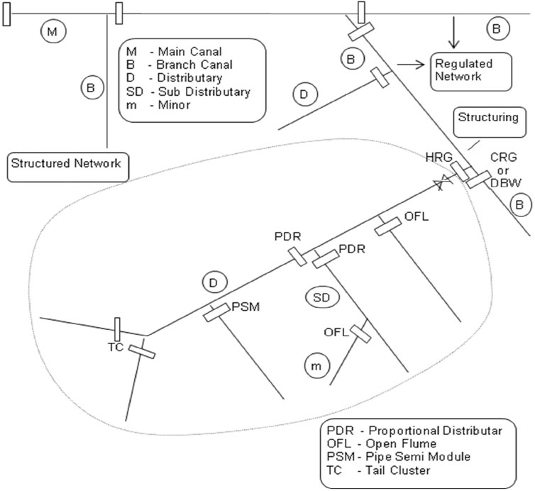
FIGURE 1. Schematic of a structured irrigation network.

The interface between the regulated part and the structured network is termed the “structuring level”. At the head of each structured network (distributary), a flow-measurement structure may be installed to verify that the structured sub network or distributary carries the allotted discharge. Once the allotted discharge is ensured at the head of the distributary, the ungated control structures at the offtakes from the distributary ensure that offtakes and outlets carry their respective allotted discharge. These ungated flow-rate control structures are of a few standard types, designed based on some standard guidelines (Sridharan and Mohan Kumar, 1996).

Choice of Network Analysis Method

The network-analysis problem considered here is as follows. In a canal network such as shown in Figure 2, at the head of the system indicated as head works (HW) in the figure, a specified flow is allowed. The layout of the canal network and the details of the individual canals, such as bed width, side slope, bed slope and Manning’s n, are specified. Also, the details of the parent canal and the offtake canal control structures are specified, besides any other structures in different reaches of the canal network. In addition, junction nodes are present where a canal bifurcates into two (Figure 2). It is obvious that in each individual canal of the network, the analysis will be based on a gradually-varied flow equation, possibly modified to account for seepage and other losses. In dealing with the complexity of the unknown discharge distribution, three broad approaches, such as direct methods (Schulte and Chaudhry, 1987; Sen and Garg, 2002), sweep methods (Mishra, 1993) and the method of Initial-Value Problem (IVP) and Boundary-Value Problem (BVP) with reconciling boundary conditions at junctions (Naidu et al., 1997) are possible. All these methods were found to be simple to implement for irrigation-canal-network analysis. In this study, iterative method proposed by Naidu et al. (1997), is chosen as the solution method.

FIGURE 2

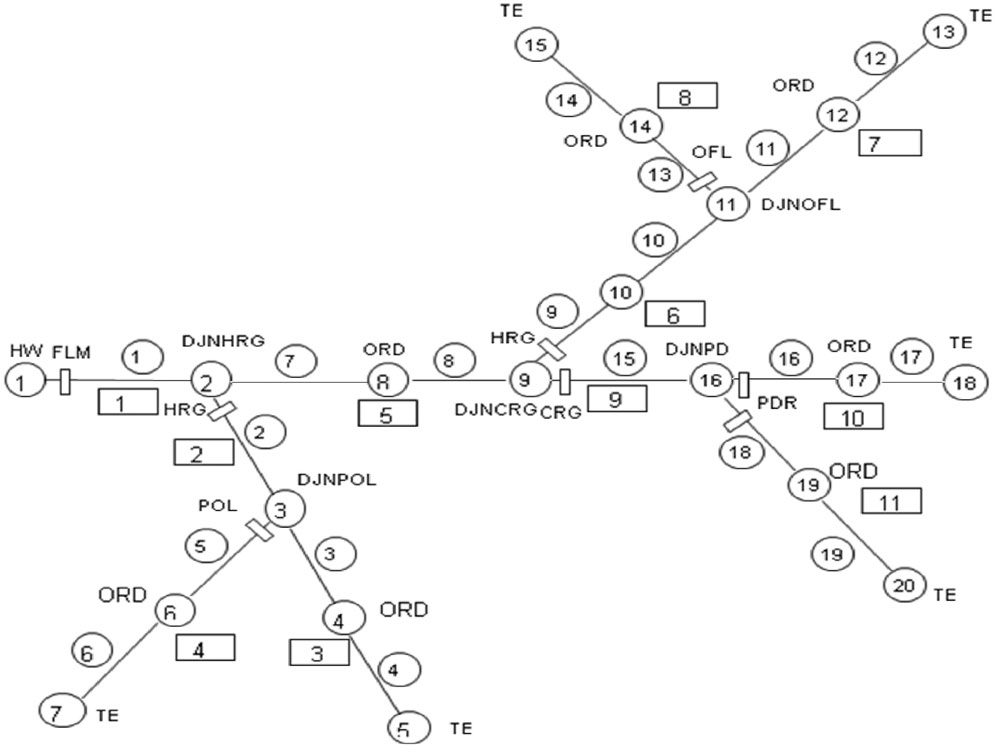
FIGURE 2. Example network.

Modified Network Analysis Model

However, for application in an actual canal network, the method proposed by Naidu et al. (1997) requires several modifications. These modifications are necessitated by the following factors: 1) At all junctions, there should be control structures; these structures can be present only in the offtake canal or in both the parent canal and the offtake canal. 2) The control structures can operate under a free (modular) condition or under a submerged (non-modular) condition; the operating condition is not known a priori and forms part of the solution. 3) There may be unstable situations at the head regulator type of offtake structure when the flow may occur in the boundary between free and submerged flow, which may require special handling. 4) As it is possible that canal sections may change significantly at several junctions, it is desirable to apply the energy equation when also taking into account the velocity head; some complications to be dealt with in this respect will be discussed subsequently. 5) Provision must be made to deal with distributed loss of water, such as seepage. 6) The real problem in the canal network will require use of the depth-discharge relationship as the boundary condition at the tail ends instead of at a specified depth—that is, in the iterative process, the depth at all the tail ends that keep changing. 7) The canal section, bed slope or Manning’s n may change even within a canal reach between two junctions; this is only a matter of detail to be resolved. 8) It is desirable for the model to be developed while keeping in view the application for design; for example, determination of the throat widths of open flume outlets using the network model.

Example Network

The modified network-analysis model is now described. The network shown in Figure 2 is used as the illustrative example to explain the procedure. In the channel reach between two junction nodes, or between a junction node and a tail-end node, some intermediate nodes are also shown to signify change in canal cross section, bed slope or Manning’s n. The numbering scheme of channels and nodes as used in Figure 2 is arbitrary as defined by the user, unlike the scheme proposed by Naidu et al. (1997). There are two sequences of channel numbers: The numbers in circles refer to all the channels in the network that are prismatic, with constant bed slope and constant Manning’s n. The channel numbers in rectangular boxes refer to the channel number between two junction nodes or between a junction node and a tail-end node. These two types of reference to canal numbers are referred to as IC sequence (circle box) and JC sequence (rectangular box) canals. Thus, in the example network, there are 19 IC canals and 11 JC canals. In the example network, different types of control structures also are marked. These structures may not represent a real irrigation network and may only serve here to explain the analysis procedure.

In the network are two Type 2 nodes, as described by Naidu et al. (1997): nodes 2 and 9, which are not directly connected to a tail-end node. As a result, there will be two groups of canals requiring Group Boundary-Value Problem (GBVP) computation, comprising JC canals 6 through 8 and 2 through 4 (the corresponding IC canals are 9 through 14 and 2 through 6).

Type of Nodes and Channels

The nodes such as 4, 6, and 8 are referred to as ordinary nodes, in which there is only change in the canal cross section, bed slope or Manning’s n. At the ordinary nodes, there is no transfer of discharge into another channel, and hence the IVP computation can proceed through the ordinary node to reach a junction node. The junction nodes are categorized into various types on the basis of the type of control structures at the junction. The following categorization has been included in the model: 1) DJN (dividing junction)—a junction node with no control structure, whether in a parent canal or in an offtake canal; such a junction will not normally be used in a canal network, and the option is provided only to maintain the flexibility of the model; 2) DJNCRG—a junction node with a cross regulator in the parent canal, and a head regulator in the offtake canal; 3) DJNDBW—a junction node with a duckbill weir in the parent canal, and a head regulator in the offtake canal; 4) DJNPDR—a junction node with a proportional distributor comprising a pair of flumes in the parent canal and the offtake canal; 5) DJNDRP—a junction node with a drop at the junction; 6) DJNPOL—a junction node with a pipe outlet on the offtake canal, and no structure in the parent canal; 7) DJNHRG—a junction node with a head regulator in the offtake canal, and no structure in the parent canal; 8) DJNOFL—a junction node with an open flume in the offtake canal, and no structure in the parent canal; 9) DJNPSM—a junction node with a pipe semi-module in the offtake canal, and no structure in the parent canal. In addition, node 1 at the head works, and the tail-end nodes such as 5, 18, 20, are referred to as HW and TE, respectively.

All the channels are categorized as either “parent” or “offtake.” This classification is advantageous in handling the boundary conditions when the computation reaches the upstream end of a parent canal or an offtake canal. In the example network in Figure 2, the parent canals (in terms of JC canals in rectangular boxes) are 1, 3, 5, 7, 9 and 10; the offtake canals, again in terms of JC canals, are 2, 4, 6, 8 and 11.

Computational Path

The computational path that defines the order in which the gradually-varied flow computation will be done through the network is decided following the procedure proposed by Naidu et al. (1997). The underlying concept is to minimize the iterative computations such as Group Boundary-Value Problem, GBVP and BVP. The order of computation is given in terms of the JC channels marked in rectangular boxes in Figure 2, along with the type of computation as follows: 1) channel 10, IVP; 2) channel 11, BVP; 3) channel 9, IVP; 4) channels 7, 8, 6 in that order as GBVP; 5) channel 5, IVP; 6) channels 3, 4, 2 in that order as GBVP; 7) channel 1, IVP. In IVP for a channel with a TE node (example: JC channel 10), the boundary condition at the tail end, in terms of the depth/discharge relation, is used for the computation of depth for an assumed or updated discharge. For IVP for an intermediate channel (example: JC channel 9), the depth at the downstream end is obtained from the junction boundary condition applied after a gradually-varied flow computation for the downstream channels. The junction-boundary condition will depend on the type of junction node.

For BVP in a channel with a TE node, the depth - discharge relation at the tail-end node is used for getting the depth at the downstream end for the current discharge. In the method of Naidu et al. (1997), the depth at the upstream end of the BVP channel is obtained on the basis of the junction boundary condition after the computation for the parallel channel (example: depth at the upstream end of JC channel 8 is obtained from the boundary condition at junction node 11, after a gradually-varied flow computation for JC channel 7). This procedure must be modified for a canal-network model. The computed flow condition at the upstream end of JC channel 7 can be used to calculate the flow condition at the downstream end of JC channel 6, but it cannot be used to calculate the flow condition in JC channel 8 across the open-flume outlet. Hence, in BVP computation, the reference depth for checking convergence is shifted to the parent canal upstream of the junction. In the iterative IVP computation for a BVP channel, and after the computation reaches the upstream end of the channels, the boundary condition of the offtake control structure is used to calculate the depth upstream of the junction in the parent canal. This depth is compared with the reference depth at the location where it has already been calculated.

Computation Algorithms

The computation algorithm is now described for the example network in Figure 2. An initial estimation of discharge is given for all the channels. This estimate can be arbitrary, or it may be the design discharge for the particular operating condition of the canal network. Unlike the method of Naidu et al. (1997), in which the velocity head is ignored in the junction-boundary condition, in the present method, the energy equation, including the velocity head, is applied, and hence a starting assumption for the discharge in all the channels is necessary. Initially, the assumption need not even satisfy the continuity equation at the junctions; when in the first outer iteration, the discharges will be reset to satisfy the continuity equations.

The computation starts with an assumed discharge at TE node 18 and the depth at the node is calculated using the depth-discharge relationship at the node (example: uniform-flow formula). The computation proceeds to the upstream end of JC channel 10 (node 16), taking into account the change in channel features at node 17. Junction node 16 is of the DJNPDR type with a rectangular flume in both the parent and offtake canals. As JC channel 10 is the parent canal, the discharge equation for the parent-canal flume is the boundary condition to be applied. It is assumed, that the flume functions under free or modular flow. The governing equation for the open-flume outlet can be written as follows:

$Q\left(16\right)-\frac{2}{3}\sqrt{\frac{2g}{3}} C_d b H_u^{\frac{3}{2}}=0 (1)$

where $Q\left(16\right)$ is the discharge in IC canal 16, $C_d$ is co-efficient of discharge and ‘b’ is throat width of flume:

$H_u=y_d\left(15\right)-p+\frac{V_d^2\left(15\right)}{2g}(2)$

where $y_d\left(15\right)$ is flow depth downstream of IC canal 15, ‘p’ is the crest height of the flume with respect to the parent canal bed level and $V_d\left(15\right)$ is the approach flow velocity downstream of IC canal 15. The total head $H_u$ is given by Eq. 2, and Eq. 1 provides a nonlinear equation for the depth in the upstream canal (IC canal 15). In the calculation, the velocity head in the upstream canal is based on the assumed or current estimate of discharge in IC canal 15. The $C_d$ value is considered a variable with $H_u\left(16\right)/L$.

It may be noted that as free flow is assumed over the flume, the $H_u$ value, and hence $y_d\left(15\right)$, is not dependent on the depth $y_u\left(16\right)$ calculated from the IVP; $y_u$ and $y_d$ refer to the flow depth at the upstream and downstream ends of the respective canals. However, it must be verified that the free-flow assumption is correct. For this, the submergence ratio is checked on the basis of $y_u\left(16\right)$ obtained from the IVP calculation for JC channel 10, with $y_d\left(15\right)$ calculated on the basis of Eq. 1 and the crest height of the flume. If the submergence ratio exceeds the modular limit, the flow is non-modular, and the proportional distributor is considered a head-loss structure. Now the energy equation is used to solve $y_d\left(15\right)$ from the following equation:

$CB{L}_d\left(15\right)+y_d\left(15\right)+\frac{V_d^2\left(15\right)}{2g}=CB{L}_u\left(16\right)+y_u\left(16\right)+\frac{V_u^2\left(16\right)}{2g}+K\frac{V_u^2\left(16\right)}{2g}(3)$

where subscript ‘d’ refers to the downstream end of the respective canal, subscript ‘u’ refers to the upstream end of the respective canal, CBL is canal bed level and K is the head-loss coefficient for the submerged proportional distributor. As the terms on the right side of the equation are known (as IVP is already completed for channel 16), Eq. 3 forms a nonlinear equation for $y_d\left(15\right)$.

The computation proceeds next with JC channel 11 with BVP computation. However, unlike the method of Naidu et al. (1997), the depth $y_u\left(18\right)$ cannot be determined from the boundary condition at junction node 16. Instead, the reference point for the convergence check for BVP shifts to the upstream channel, namely $y_d\left(15\right)$, which has been already computed. For all BVP computations, the reference for the convergence check is upstream of the junction. The BVP computation for JC canal 11 can start with an assumed discharge, and the depth $y_u\left(18\right)$ is arrived at by IVP computation. Now the boundary condition for the offtake canal flume in the proportional distributor is used to calculate the depth of the upstream or parent canal, namely $y_d\left(15\right)$. This computation is as already explained for the case of the flume in the parent canal. If the depth $y_d\left(15\right)$ does not match the depth already arrived at from the JC 10 computation, the discharge in JC 11 is modified, and the computation repeated, until convergence. However, it can be noted that when BVP is applied for an offtake canal, if free flow is assumed through the offtake control structure, the first assumption of discharge may be made on the basis of the depth upstream of the junction already calculated. If the flow condition turns out to be free, there is no need for iteration of the discharge in BVP computation. Thus, for open-flume offtake control structures or proportional distributors, BVP normally will not involve iteration, as flow is likely to be free. However, for offtake control structures such as pipe outlets, which are normally submerged, iteration will be needed. The algorithm is general, which recognizes that iterative computation may be needed for BVP.

Once the downstream JC canals 10 and 11 are solved, the discharge in JC 9 is obtained by the continuity equation. As $y_d\left(15\right)$ and Q are known, IVP is applied to JC 9. At junction node 9, there is a cross regulator in the parent canal, and a head regulator in the offtake canal. First, the cross-regulator boundary condition is treated as a head-loss structure condition similar to Eq. 3), and $y_d\left(8\right)$ is solved from the energy equation. If $y_d\left(8\right)$ is less than FSD (8), $y_d\left(8\right)$ is set to FSD; that is, it is assumed that the cross-regulator gate will be set so as to maintain water level upstream of the regulator at full supply depth. If calculated $y_d\left(8\right)$ is greater than FSD (8), the calculated depth is retained (the assumption is that freeboard is not exceeded).

With $y_d\left(8\right)$ known, JC canals 7, 8, 6 are solved as a GBVP problem. As in the case of BVP, the reference point for the convergence check for the GBVP problem is $y_d\left(8\right)$ upstream of the junction, and not $y_d\left(9\right)$ as in Naidu et al. (1997). In the GBVP set, JC 7 is an IVP canal, JC 8 is a BVP canal and JC 6 is an IVP canal. It can be noted that offtake canal JC 8 is a BVP canal instead of parent-canal JC 7, as the open-flume structure that may function as a free-flow control structure makes the BVP solution practically non-iterative. The computation for the group of canals starts with an assumed discharge Q 12) and $y_d\left(12\right)$ calculated from the tail-end boundary condition. IVP is applied for JC 7 to obtain $y_u\left(11\right)$. At junction node 11 the energy equation is applied for calculating $y_d\left(10\right)$. Ignoring energy loss at the junction, the equation is given by:

$CB{L}_d\left(10\right)+y_d\left(10\right)+\frac{V_d^2\left(10\right)}{2g}=CB{L}_u\left(11\right)+y_u\left(11\right)+\frac{V_u^2\left(11\right)}{2g}(4)$

In all these junction equations, the velocity head upstream of the junction is based on the current estimate of discharge.

Now BVP is applied for JC 8, using $y_d\left(10\right)$ as the reference check for convergence. Once Q (13) is obtained, Q (10) is obtained from the continuity equation. With Q (10) and $y_d\left(10\right)$ known, IVP is applied for JC 6, and $y_u\left(9\right)$ is obtained. With $y_u\left(9\right)$ known, the boundary condition at the head regulator is applied to get $y_d\left(8\right)$. The head across the head regulator is calculated from the following equation:

$Q\left(9\right)-C_d A_V \sqrt{2gh}=0(5)$

where $C_d$ is the co-efficient of discharge, $A_V$is the area of vent opening and h is the operating head. The operating head differs for free and submerged flows. For submerged flow, h is given by $\left(y_d\left(8\right)-y_u\left(9\right)\right)$, where $y_u$ and $y_d$ refer to the flow depth at the upstream and downstream ends of the respective canals, while for free flow, h is given by $\left(y_d\left(8\right)-\text{δ w}\right)$, where $\text{w}$ is sluice opening height and $\text{δ}$ is contraction co-efficient whose value may be taken as 0.62 (Bos et al., 1975). The value of $C_d$ is 0.6–0.61. If flow is free then the following equation is satisfied (Bos et al., 1975):

$\frac{y_u\left(9\right)}{w}<\frac{\delta }{2}\left[\sqrt{1+16\left[\frac{H_d\left(8\right)}{\delta w}-1\right]}-1\right](6)$

Initially the computation assumes that the head regulator has free flow, and $y_d\left(8\right)$ is calculated accordingly. Then Eq. 6 is used to verify whether the head regulator functions under a submerged condition. If so, $y_d\left(8\right)$ is modified on the basis of the canal bed levels in the parent canal and offtake canal and $y_u\left(9\right)$, and the calculated head across the head regulator. The value of $y_d\left(8\right)$ obtained by this procedure is compared with $y_d\left(8\right)$ obtained earlier from applying the junction boundary condition at node 9 from JC channel 9. If there is a difference, Q (12) is modified, and the entire computation for the group of JC canals 7, 8, 6 is repeated.

With Q (8) and $y_d\left(8\right)$known, IVP is applied for JC 5 to obtain $y_u\left(7\right)$. The energy equation at junction node 2 is used to calculate $y_d\left(1\right)$. Now JC canals 2, 3, 4 are to be solved by GBVP computation. As JC 4 is the offtake canal with a pipe outlet as the control structure, JC 3 is considered as the IVP canal, and JC 4 as the BVP canal. Q (4) is assumed, and IVP is applied to get $y_u\left(3\right)$; and the junction energy equation is applied to get $y_d\left(2\right)$. BVP is applied for JC 4, starting with an assumed discharge and iterating until convergence is achieved for $y_d\left(2\right)$. As a pipe outlet normally functions under a submerged condition, iterations may be required for the BVP solution. Now the IVP is applied for JC channel 2, and with $y_u\left(2\right)$ and the head regulator boundary condition, $y_u\left(1\right)$ is calculated. A convergence check for the GBVP problem is made on the basis of the prior estimate of $y_u\left(1\right)$. On this basis, Q (4) is modified for the GBVP iteration.

Thus, knowing Q (2) and Q (7), Q (1) is obtained. This procedure completes one outer iteration. If the value of Q (1) does not match the discharge released at the head works, the entire computation is repeated by changing the discharge Q (17), that is, node 18, which is the starting node in the computational path. Once convergence is achieved, the gradually-varied flow computation can proceed through IC canal 1 to obtain the depth up to the head works. The algorithm for the example network is summarized in the pseudo-code given in Figure 3. In the figure, all canal numbers refer to IC canals, that is circles in Figure 2.

FIGURE 3

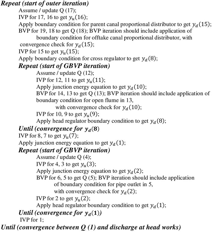
FIGURE 3. Pseudo code for computational algorithm for example network.

Details of Computational Algorithms

Data Structure

The layout of the canal network is defined by giving data for the number of canals, the number of nodes, for each canal upstream and downstream node number and for each node, type of node and predecessor and successor canal numbers. If there is some redundancy in the data, it is verified for consistency. For each canal the type of canal (parent or offtake canal), length, bed width, side slope, Manning’s n, bed slope, start chainage, bed level at the start and seepage-loss constant are provided. In addition, the design discharge is also provided for each canal to enable calculation of full supply depth as well as to compare actual flow of water “vis-à-vis” design discharge. Subroutines are prepared to identify upstream and downstream canals readily at any node. Data for all types of structures are given in serial-number format (for example, NCRG cross regulators, NPOL pipe outlets etc.). For each serial number, for each type of structure, the location is to be identified in terms of canal number and chainage. In addition, depending on the type of structure, additional data are required. For example, for a duckbill weir, the crest height, number of cycles, length of crest per cycle, sluice area, drop height (if any), coefficient of discharge for the weir, coefficient of discharge for the sluice and head-loss coefficient for submerged flow conditions are to be provided. For a pipe outlet, the number of pipes, diameter of pipe, length of pipe, setting of pipe invert above bed level, type of entry and constriction sleeve (if any) are to be provided. For many structures that may operate under free or submerged flow conditions, the modular limit may have to be provided as additional data unless general guidelines such as σc = 0.8, as used for open flumes, are included as part of the code. The discharge allowed at the head works is the required data for a particular simulation.

At all computational nodes, two depths are stored, $y_{us}(ic,in)$ and $y_{ds}(ic,in)$, where $\mathit{ic}$ refers to canal number and $\mathit{in}$ refers to node number within the canal. This is done because there may be several nodes where there are structures (example: bridge) where the depth upstream and downstream of the node may vary. It can be noted that $\mathit{in}$, referred to above, is different from the junction nodes discussed so far with respect to figures such as Figure 2.

Discretization

The individual canals are to be segregated into reaches, with interior computational nodes for gradually-varied flow computation. For this, the structures in the individual canals are first sorted and cataloged in ascending order of chainage from the beginning of the canal. The discretization is done to ensure that a computational node is located at each structure; besides, the maximum spacing allowed between two nodes is also specified. These criteria are used in the discretization scheme.

Computational Path

The computational path is decided on the basis of the guidelines provided by Naidu et al. (1997), keeping in view the need to minimize iterative computations such as GBVP and BVP. Taking advantage of the possibility of free flow occurring at offtake control structures, which may avoid iterative computations for BVP as much as possible, offtake canals are organized as BVP canals. The algorithm keeps in view the possibility of GBVP computation as a nested loop, such as the example shows in Figure 4. The GBVP for canals 5, 6 and 7 occurs nested within the GBVP computation for canals 4, 8, 9 and 10.

FIGURE 4

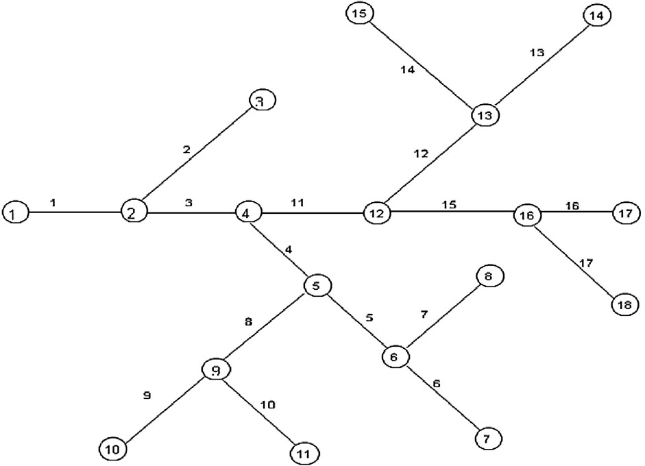
FIGURE 4. Example network showing GBVP in nested loop.

IVP Computation

The fourth-order Runge-Kutta method is used for gradually varied flow computation, involved in the lowest level computation of the algorithm. However, the results are also verified for the application problem by solving the finite-difference equation for gradually-varied flow by the Newton method in each step. These algorithms are summarized below. The general equation with seepage loss is considered as follows:

$\frac{dy}{dx}=\frac{S_o-S_f-\left(\frac{\alpha Q{q}^{\ast }}{g{A}^2}\right)}{1-\left(\frac{\alpha Q^2}{g{A}^{2}D}\right)}(7)$

where y is the flow depth, x is the distance along the channel, $S_o$is the bed slope, $S_f$ is the friction slope, Q is the discharge in the channel, A is the cross-sectional area, D is the hydraulic depth, q* is the seepage discharge in the channel and $\alpha$ is kinetic energy coefficient.

Runge-Kutta Method

The computation proceeds from a downstream section to the next upstream section, as flow is subcritical. The R-K method for calculating the depth of the upstream section is as follows:

$y_{i-1}=y_i+\frac{1}{6} \left[a_1+2a_2+2a_3+a_4\right](8)$

where

$a_1=\Delta xf(x_i,y_i)$

$a_2=\Delta xf(x_i+\frac{\Delta x}{2},y_i+\frac{a_1}{2})$

$a_3=\Delta xf(x_i+\frac{\Delta x}{2},y_i+\frac{a_2}{2})$

$a_4=\Delta xf(x_i+\Delta x,y_i+a_3)$

$\Delta x=x_{i-1}-x_i$ and function f is given by the right side of Eq. 7.

The value of $y_{i-1}$, calculated as above, refers to $y_{ds}(ic,in-1)$. If the computational node is an ordinary interior node, $y_{us}(ic,in-1)$ = $y_{ds}(ic,in-1)$. If there is a structure at the $(in-1)$ node, the boundary condition at the structure must be applied for calculating $y_{us}(ic,in-1)$ from $y_{ds}(ic,in-1)$. For example, if there is a road bridge (which is treated as a head-loss structure in the model), the energy equation is to be solved by the Newton method to calculate $y_{us}(ic,in-1)$. If there is a measuring flume, the equation for discharge over the flume has to be used. If the flume operates under a free-flow condition, $y_{us}(ic,in)$ does not depend on $y_{ds}(ic,in)$. If the flume operates under a submerged condition, the energy equation that accounts for head loss can calculate $y_{us}(ic,in)$ from $y_{ds}(ic,in)$.

In order to handle seepage loss, an iterative approach is used. The discharge at the downstream section is used in the gradually-varied flow equation without considering seepage loss. Once the depth at the in-1 section is calculated, the average depth in the reach in to in-1 is used to calculate the wetted perimeter. The seepage loss in the reach in to in-1 is specified in terms of the wetted perimeter by the following equation:

$\Delta Q_s=S_c\ast \overline{P}\ast \Delta x(9)$

where $\Delta Q_s$ is the seepage loss in the reach in to in-1, $\overline{P}$ is the average wetted perimeter in the reach, $\Delta x$ is the distance between the in and in-1 nodes and $S_c$ is the seepage loss constant, which may be specified separately for each canal. Thus, the wetted area in the reach in to in-1 is used to calculate seepage loss, and the discharge at in-1 is obtained by adding seepage loss to the discharge at in. Now, the average discharge in the reach in to in-1 is used, and Eq. 8 are again used to calculate $y_{ds}(ic,in-1)$. Normally, one such iteration is adequate, but if the seepage and other losses are considered excessive, the option for additional iterations is provided in the algorithm.

Newton Method

The Newton method for the solution of the IVP problem is used only for verification of the result from the Runge-Kutta method for selected cases. The finite-difference approximation of Eq. 7 is written as:

$\frac{y_i-y_{i-1}}{x_i-x_{i-1}}=\frac{S_o-\overline{S_f}-\left(\frac{\alpha \overline{Q}{q}^{\ast }}{g{\overline{A}}^2}\right)}{1-\left(\frac{\alpha {\overline{Q}}^2}{g{\overline{A}}^2\overline{D}}\right)} (10)$

where

$S_o=Bed slope of the channel$

$\overline{S_f}=\frac{S_{f i}+S_{f i-1}}{2}=Average energy slope between two section$

$\overline{Q}=\frac{Q_{ i}+Q_{ i-1}}{2}=Average discharge between two section$

$\overline{D}=\frac{D_{ i}+D_{ i-1}}{2}=Average hydraulic depth between two section$

$\overline{A}=\frac{A_{ i}+A_{ i-1}}{2}=Average cross sectional area between two section$

Eq. 10 is a nonlinear equation in the unknown yi-1. An iterative procedure by the Newton method can be used to solve yi-1, which corresponds to $y_{ds}(ic,in-1)$. Once $y_{ds}(ic,in-1)$ is calculated, $y_{us}(ic,in-1)$ is calculated as explained for the Runge-Kutta method.

Updating Discharge in Iterative Computation

There are three levels at which the discharge may have to be updated in the iterative computation. In the outermost iteration the discharge at the beginning tail-end canal (that is, the first canal in the computational path) is varied, based on comparison between the computed and the actual discharge at the head works. At the second level the discharge at the starting canal of a GBVP computation has to be varied on the basis of depth comparison with the parent canal upstream of the junction at the head of the group BVP canals. At the third level the discharge in a BVP canal may have to be varied on the basis of depth comparison at the junction node upstream of the BVP canal. Naidu et al. (1997) proposed an extrapolation scheme based on a shooting method for updating the discharge in the iterations. As this may lead to a spurious negative discharge or a Froude number exceeding unity, these authors proposed methods to condition the iterations. As the present application involves a large variety of structures that can function under free or submerged flow conditions, it was felt desirable to keep the computations robust, even at the cost of computational time. Besides, in the present study, some inferences are also drawn from the results at intermediate iterations, as will be seen subsequently. The numerical-conditioning approach for the iterations may give distorted results at intermediate iterations. Considering all these factors, the following direct-search approach is used for updating the discharge in the iterative computation.

An initial value of ΔQ as a fraction of the current discharge (10% is used at the start) is specified. When the discharge has to be increased or decreased, this value is used in the iteration. As the iteration proceeds, the discharge may overshoot the correct value, which is reflected by change in the direction of correction. Whenever such overshooting occurs, the discharge correction ΔQ is halved. The iteration continues until ΔQ becomes sufficiently small. The convergence check is based on depth comparison as explained in the network algorithm (section 2.6) as well as on ΔQ. With this approach, although the computation may take more time, there will be no occurrence of negative discharge, and in most canal applications the Froude number also will not exceed unity. In fact, it was verified that convergence was obtained (Figure 5), with a very poor initial value of discharge, at the beginning canal of the computational path. Table.1 Shows channel characteristics and solution for example network in Figure 2.

FIGURE 5

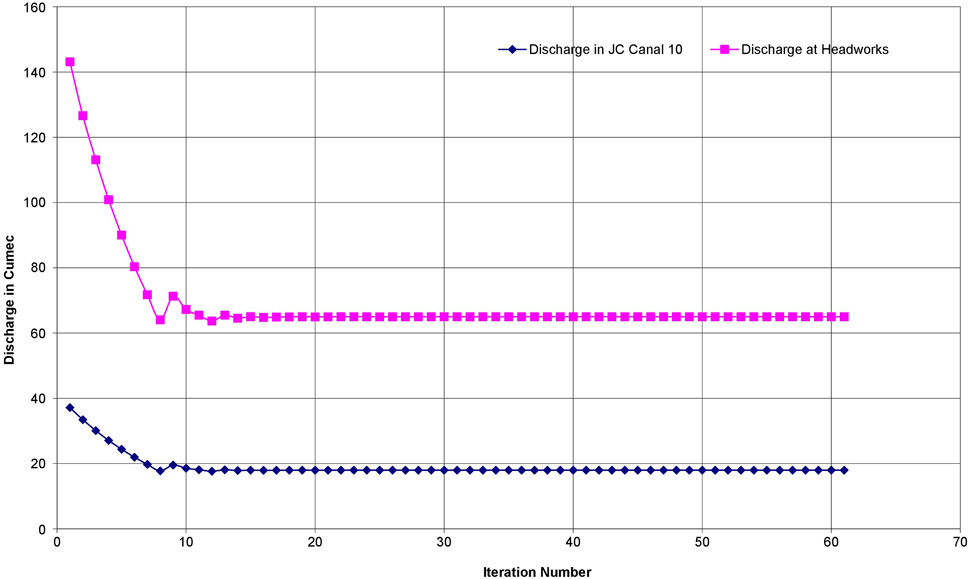
FIGURE 5. Convergence characteristic for initial assumption in JC Canal 10 at design discharge.

TABLE 1

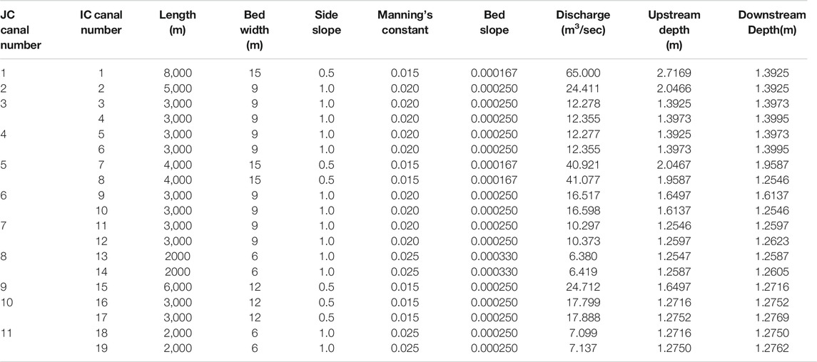
TABLE 1. Channel characteristics and solution for illustrative example network in Figure 2.

Additional Computational Issues

In view of the conservative procedure for updating discharge are described in Updating Discharge in Iterative Computation, there has been no problems of over shooting of the solution, resulting in negative discharge or Froude number more than unity. However, there were some other issues to be dealt with. Occasionally, it was found that the energy level downstream of a junction was such that, with respect to the upstream canal cross section and discharge, it was less than the energy level corresponding to critical flow. In such a case, the energy equation at the junction either does not converge or gives spurious negative depth values. Hence in applying the energy equation at the junction, it is first verified whether the energy is above that required for critical flow, that is above the minimum energy level for the upstream canal. If so, the computation proceeds to solve the energy equation to find the upstream depth. If not, the energy level on the upstream side of the junction is set corresponding to critical flow and the upstream depth solved. In some situations, the computation was shifting from free to submerged flow (head regulator). If such a situation occurs, it is identified in the computation and the flow is set to submerged flow. Actually, in such a situation, the flow will be oscillating, with the hydraulic jump moving away from the gate ensuring free flow and then moving back to the gate resulting in submerged flow.

Result Analysis

Model Adaptation for Design and Operation

Design Application

The problem of design as posed for the structured irrigation network is the design of offtake control structures, mainly open flume and pipe semi-module. The design is to be accomplished so as to achieve the desired discharge distribution among the different canals. This procedure is explained through the example network considered earlier, but this time with open flume outlets as the control structures at offtakes. This is shown in the network presented in Figure 6. In addition to the canal details, such as bed width, side slope, bed slope, Manning’s n and length, the design discharge at the headworks and the required discharge distribution in all the offtake canals are specified. In the design algorithm using the network model, the throat width of the open flume is computed, with the crest height specified.

FIGURE 6

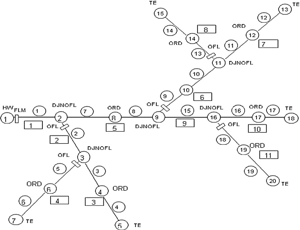
FIGURE 6. Example network with open flume outlets.

The computation starts with JC canal 10 from node 18 as before. But instead of assuming the discharge, the design discharge in IC canal 17 is used in the IVP computation. Once $y_u\left(16\right)$ is obtained from IVP for canal 17, 16, the junction energy equation is applied at node 16 to get $y_d\left(15\right)$. Now the computation proceeds with JC canal 11, with the design discharge in IC canal 19. The tail-end boundary condition yields the depth at node 20, and the IVP computation is done for IC canals 19, 18 to get $y_u\left(18\right)$. Now the flow condition upstream of junction node 16 is known, based on $y_d\left(15\right)$ already calculated. Discharge Q (15) is the design discharge in the canal, as the discharges in canals 16 and 18 are the respective design discharges. The condition on either side of the open flume is known. Hence, it can be verified that the flow over the flume is modular; if it is non-modular (owing to a high submergence ratio), the crest height of the flume should be increased. The total head over the flume can be calculated, and the flume equation, Eq. 1 can be used to solve the throat width, b_o.

The computation proceeds with IVP for JC canal 9 to get $y_u\left(15\right)$. As the design algorithm will ensure design flow in all the canals, the discharge in canal 8 is the design discharge. The energy equation at junction node 9 gives $y_d\left(8\right)$. IVP is now applied for JC canal 7, with the design discharge in IC canal 12 and tail-end depth as calculated from the boundary condition. Once $y_u\left(11\right)$ is calculated, the junction equation at node 11 yields $y_d\left(10\right)$. The discharge in IC canal 14 is established as the design discharge, and IVP is done for 14, 13 to get $y_u\left(13\right)$. Knowing the flow conditions on either side of the open flume in offtake canal 13, the flume width is calculated as before. The computation proceeds with IVP for JC canal 6 to get $y_u\left(9\right)$. Now, the throat width of the open flume at offtake canal 9 can be calculated. Next, computation proceeds with IVP for JC canal 5 to get $y_u\left(7\right)$. The energy equation at node 2 gives $y_d\left(1\right)$. The open flumes in offtake canals 5 and 2 are designed as already explained for the group of canals 9 through 14. Thus, computation can be completed with IVP for IC canal 1 if required, although it is not necessary for the design problem.

For the pipe semi module, the approach is practically the same except that the water level in the exit tank first must be calculated from the depth upstream of the junction and the design discharge, based on the pipe-outlet loss. Then this water level is used for calculating the head over the flume and designing the throat width of the flume. For a proportional distributor, whatever the choice of crest height and throat width might be, the design of the two flumes is such as to ensure flows proportional to the design flows in the parent canal and the offtake canal, once the design discharge is ensured at other outlets such as open-flume and pipe semi-module outlets. Thus, the design discharge is automatically ensured at the proportional distributor. However, if a specific depth is desired in the upstream canal (example: full supply depth), the network model can be used for deciding the throat width of the two flumes in the proportional distributor as well.

It may be noted that the design solution is non-iterative, unlike the analysis solution. Normally, in a structured irrigation network, each offtake control structure will be designed in a stand-alone based on the uniform-flow concept. If any backwater effects are present because of various structures in the canal, this approach will not be able to account for them. In the present case, through the network model, the design of all the offtake structures is completed simultaneously, besides accounting for any backwater effects that may be in the system.

Model Application in Operation

Design application is proposed for the offtake control structures in the structured irrigation network. The operation application is proposed for a traditional system with pipe outlets and head regulators as the offtake control structures and the objective here is to determine the head-loss coefficient required for the pipe outlet, or the gate opening required for the head regulator, in order to limit the discharge to the design discharge. Also, the head-loss coefficient may be used to determine the extent of closing required at the pipe-outlet gate. If the extent of such throttling required is very high, it is obvious that there will be a strong resistance from the farmers.

The procedure is similar to the design application for a structured irrigation network. In Figure 6 the open flumes may be looked upon as pipe outlets for this purpose. The computation reaches $y_d\left(15\right)$ through IVP for JC canal 10, by applying the junction energy equation at node 16. IVP is applied for JC canal 11 with design discharge to get $y_u\left(18\right)$. On the basis of this value, it is decided whether the pipe outlet functions under a free or a submerged condition. The head across the outlet is known, as $y_d\left(15\right)$ and $y_u\left(18\right)$ are known. The head loss for a full open-pipe outlet can be calculated, and the difference between the two values provides the basis for calculating the additional-loss coefficient required. If this value is negative, the implication is that the pipe outlet is under-designed and cannot carry the designed discharge. If this value is positive, the extent of the opening of the gate has to be established on this basis. In practice, managing the gate opening of the pipe outlet at different discharges has posed considerable problems, and this is the motivation for the development of the concepts underlying the structured irrigation network. However, the model can be applied to an actual system to study the nature of the problem. This is also a non-iterative computation. The approach is similar at a head regulator for determining the extent of the gate opening. For deciding the nature of flow (free or submerged) for a head regulator, the criterion given by Eq. 6 is to be used.

Software Development

A program has been developed in FORTRAN for implementing the canal network algorithm. The program is about 2,600 lines (excluding commentary statements) with a main program and 32 subroutines. The major subroutines are 1) a discretization module, in which the computed nodes are fixed, and the locations and associated characteristics of different structures are related to the computational nodes; 2) a module specifying the computational path; 3) a main computational module of IVP, BVP and GBVP along the specified computational path; 4) a GBVP module (a recursive subroutine to allow for GBVP computation in a nested loop); 5) a BVP module; 6) an IVP module; 7) a cluster of modules for different types of control and other structures; and 8) output modules for flow distribution, water-surface profiles, flow depth etc.

Conclusion

• The canal-network model, as developed and used in this study, is described. The algorithm is described through an example network with different types of control structures in it. The basic analysis procedure is based on the iterative approach proposed by Naidu et al. (1997). However, several modifications had to be introduced in the method so as to make it applicable analysis for traditional and structured irrigation networks.

• The model as developed can be applied to any canal network, either major irrigation systems or compact sub-systems such as structured irrigation networks. A FORTRAN program has been developed to implement the algorithm.

• The analysis model is modified to handle design problems in structured irrigation networks and operational problems in traditional irrigation networks.

• The focus in this research is the efficacy of the water management in ensuring equitable distribution of flow at different discharges released at the head works. For this, both traditional infrastructure for flow distribution and infrastructure as per structured irrigation networks concept are studied.

Data Availability Statement

The datasets presented in this study can be found in online repositories. The names of the repository/repositories and accession number(s) can be found in the article/Supplementary Material.

Author Contributions

GVF Computation in Structured Irrigation Networks SS as author: The data collection, analysis of the data and as per the conceived objectivities, the research was carried out and the paper was written by the author. KS as Co-author: Under his supervision SS completed his PhD.

Conflict of Interest

The authors declare that the research was conducted in the absence of any commercial or financial relationships that could be construed as a potential conflict of interest.

Publisher’s Note

All claims expressed in this article are solely those of the authors and do not necessarily represent those of their affiliated organizations, or those of the publisher, the editors and the reviewers. Any product that may be evaluated in this article, or claim that may be made by its manufacturer, is not guaranteed or endorsed by the publisher.

Acknowledgments

The authors sincerely thank the reviewers and the editor Prof. FP for reviewing this manuscript. The manuscript was largely benefitted by the review process. SS thank his daughter Akshaya Suresh, XII student and his wife K. Sathia Meena, Assistant Professor, GCA, Salem-5 for their constant encouragement to write this manuscript.

References

Baume, J. P., Sally, H., Malaterre, P. O., and Rey, J. (1993). Development and Field Installation of a Mathematical Simulation Model in Support of Irrigation Canal Management. Colombo, Sri Lanka: International Irrigation Management Institute.

Bos, M. G. (1975). Discharge Measurement Structures. Oxford and IBH Co.

Chaudhry, M. H. (2008). Open Channel Flow. Second edition. New York: Springer, 10013, USA. doi:10.1007/978-0-387-68648-6

CrossRef Full Text

Chaudhry, M. H., and Schulte, A. (1986a). Computation of Steady State, Gradually Varied Flows in Parallel Channels. Can. J. Civ. Engm. 13 (1), 39–45. doi:10.1139/l86-006

CrossRef Full Text | Google Scholar

Chaudhry, M. H., and Schulte, A. (1986b). Simultaneous Solution Algorithm for Channel Network Modeling. Water Resour. Res. 29 (2), 321–328.

Google Scholar

Chow, V. T. (1959). Open Channel Hydraulics. New York: McGraw-Hill.

Islam, A., Raghuwanshi, N. S., Singh, R., and Sen, D. J. (2005). Comparison of Gradually Varied Flow Computation Algorithms for Open-Channel Network. J. Irrig. Drain Eng. 131 (5), 457–465. doi:10.1061/(asce)0733-9437(2005)131:5(457)

CrossRef Full Text | Google Scholar

Mishra, R. (1993). “Analysis Parameter Estimation and Operational Control of Canal Systems,”. Ph.D. Thesis (Bangalore, India: Indian Institute of Science).

Google Scholar

Misra, R., Sridharan, K., and Mohan Kumar, M. S. (1992). Transients in Canal Network. J. Irrigation Drainage Eng. 118 (5), 690–707. doi:10.1061/(asce)0733-9437(1992)118:5(690) https://www.ias.ac.in/public/Volumes/sadh/016/01/0085-0099.pdf.

CrossRef Full Text | Google Scholar

Naidu, B. J., Bhallamudi, S. M., and Narasimhan, S. (1997). GVF Computation in Tree-type Channel Networks. J. Hydraulic Eng. 123 (8), 700–708. doi:10.1061/(asce)0733-9429(1997)123:8(700)

CrossRef Full Text | Google Scholar

Raj Kumar, S. (1997). “Studies of Offtake Control Structures in Irrigation Canals,”. M.Sc. [Engg.] Thesis (Bangalore, India: Indian Institute of Science).

Google Scholar

Reddy, H. P., and Bhallamudi, S. M. (2004). Gradually Varied Flow Computation in Cyclic Looped Channel Networks. J. Irrig. Drain Eng. 130 (5), 424–431. doi:10.1061/(asce)0733-9437(2004)130:5(424)

CrossRef Full Text | Google Scholar

Schulte, A. M., and Chaudhry, M. H. (1987). Gradually-varied Flows in Open-Channel Networks. J. Hydraulic Res. 25 (3), 357–371. doi:10.1080/00221688709499276

CrossRef Full Text | Google Scholar

Sen, D. J., and Garg, N. K. (2002). Efficient Algorithm for Gradually Varied Flows in Channel Networks. J. Irrig. Drain Eng. 128 (6), 351–357. doi:10.1061/(asce)0733-9437(2002)128:6(351)

CrossRef Full Text | Google Scholar

Sridharan, K. (1995). Guidelines on Hydraulic Design in Structured Irrigation Network—The Duckbill Weir, Training Module Prepared for World Bank. New Delhi: Department of Civil Engineering, Indian Institute of Science, Bangalore, India.

Sridharan, K., and Mohan Kumar, M. S. (1996). Studies on Structured Irrigation Networks, Technical Report Prepared for National Water Management Project. Bangalore: Department of Civil Engineering, Indian Institute of Science, Bangalore, India.

Wylie, E. B. (1972). Water Surface Profiles in Divided Channels. J. Hydraulic Res. 10 (3), 325–341. doi:10.1080/00221687209500164

CrossRef Full Text | Google Scholar

Zhang, M.-l., and Shen, Y.-M. (2007). Study and Application of Steady Flow and Unsteady Flow Mathematical Model for Channel Networks. J. Hydrodyn 19 (5), 572–578. doi:10.1016/s1001-6058(07)60155-3

CrossRef Full Text | Google Scholar

Glossary

A Cross sectional area of the channel

Av area of vent opening for head regulator

H operating head for head regulator

b throat width of the flume

C_d coefficient of discharge

CBL_u canal bed level in the parent canal upstream

CBL_d canal bed level in the parent canal downstream

cumec Cubic meter per second

D hydraulic depth

DJN junction node with no control structure either in parent or offtake canal

DJNCRG junction node with cross regulator in parent canal and head regulator in offtake canal

DJNDBW junction node with duckbill weir in parent canal and head regulator in offtake canal

DJNDRP junction node with drop at the junction

DJNOFL junction node with open flume in the offtake canal and no structure in the parent canal

DJNPDR junction node with proportional distributor comprising a pair of flumes in the parent and offtake canals

DJNPOL Junction node with pipe outlet in the offtake canal and no structure in the parent canal

DJNHRG junction node with a head regulator in the offtake canal, and no structure in the parent canal

DJNPSM junction node with pipe semi module in the offtake canal and no structure in the parent canal

FSD full supply depth

GBVP group boundary value problem

HW head works

h_d head over crest downstream of the flume

h_u head over crest downstream of the flume

ic canal number

in node number within the canal

IVP initial Value problem

n manning’s coefficient

q* seepage discharge in the channel

Q discharge in the canal

S_c seepage loss constant

S_o bed slope

S_f friction loss constant

POL pipe outlet

$\overline{P}$ average wetted perimeter in the reach

Vu velocity upstream of the junction

Vd velocity downstream of the junction

y flow depth

y_u depth upstream of the junction

y_d depth downstream of the junction

$y_{us}(ic,in)$ upstream depth at in^th computational node in ic^th canal

$y_{ds}(ic,in)$ downstream depth at in^th computational node in ic^th canal

w Width of one cycle for duckbill weir; vent opening for head regulator

x the distance along the channel

α kinetic energy coefficient

δ Contraction co-efficient

Δx distance between the in and in-1