
94% of researchers rate our articles as excellent or good
Learn more about the work of our research integrity team to safeguard the quality of each article we publish.
Find out more
METHODS article
Front. Earth Sci., 24 June 2021
Sec. Sedimentology, Stratigraphy and Diagenesis
Volume 9 - 2021 | https://doi.org/10.3389/feart.2021.659611
Machine-learning algorithms have been used by geoscientists to infer geologic and physical properties from hydrocarbon exploration and development wells for more than 40 years. These techniques historically utilize digital well-log information, which, like any remotely sensed measurement, have resolution limitations. Core is the only subsurface data that is true to geologic scale and heterogeneity. However, core description and analysis are time-intensive, and therefore most core data are not utilized to their full potential. Quadrant 204 on the United Kingdom Continental Shelf has publicly available open-source core and well log data. This study utilizes this dataset and machine-learning models to predict lithology and facies at the centimeter scale. We selected 12 wells from the Q204 region with well-log and core data from the Schiehallion, Foinaven, Loyal, and Alligin hydrocarbon fields. We interpreted training data from 659 m of core at the sub-centimeter scale, utilizing a lithology-based labeling scheme (five classes) and a depositional-process-based facies labeling scheme (six classes). Utilizing a “color-channel-log” (CCL) that summarizes the core image at each depth interval, our best performing trained model predicts the correct lithology with 69% accuracy (i.e., the predicted lithology output from the model is the same as the interpreted lithology) and predicts individual lithology classes of sandstone and mudstone with over 80% accuracy. The CCL data require less compute power than core image data and generate more accurate results. While the process-based facies labels better characterize turbidites and hybrid-event-bed stratigraphy, the machine-learning based predictions were not as accurate as compared to lithology. In all cases, the standard well-log data cannot accurately predict lithology or facies at the centimeter level. The machine-learning workflow developed for this study can unlock warehouses full of high-resolution data in a multitude of geological settings. The workflow can be applied to other geographic areas and deposit types where large quantities of photographed core material are available. This research establishes an open-source, python-based machine-learning workflow to analyze open-source core image data in a scalable, reproducible way. We anticipate that this study will serve as a baseline for future research and analysis of borehole and core data.
Supervised and unsupervised machine-learning techniques have been widely employed by petrophysicists for subsurface analysis for almost forty years (Wolff and Pelissier-Combescure, 1982), and more advanced neural networks were subsequently developed for facies prediction and petrophysical formation evaluation (Baldwin et al., 1990). Recently, the increased accessibility of modern machine-learning (ML) methods and digital data-collection efforts have led to a resurgence of ML research for surface and subsurface characterization (Dramsch, 2020). In 2016, the Society of Exploration Geophysicists organized a ML contest to predict facies from a core-calibrated well-log dataset (Hall, 2016). Participants used various models, including k-nearest neighbors, neural networks, support vector machines, and boosted tree models (Hall and Hall, 2017), with the most accurate model utilizing a boosted tree approach with a median accuracy of 0.64 from nine classes (Hall and Hall, 2017). The dataset provided in the contest is still being used today for new ML-based facies prediction studies (e.g., Dunham et al., 2020). This contest demonstrated that well log data is a powerful data type for ML-based lithology and facies prediction, but logs are low-resolution data, typically only resolving vertically ∼0.3 m for gamma ray, ∼0.5 m for density, and ∼0.1 m for photoelectric tools (Rider and Kennedy, 2011). Resolving fine-scale (<5 cm) changes in lithology using standard log data is impossible (Passey, 2006), preventing well-log data from fully characterizing the subsurface. This log-resolution limit is a key reason that core data are collected and analyzed, as core and/or cuttings are necessary to fully resolve fine-scale changes in lithology as well as other subsurface geologic characteristics [e.g., sedimentary structures, grain size, bioturbation (Tucker, 2012)].
Slabbed geologic core, primarily collected during drilling for hydrocarbon exploration and development, is expensive to collect and store, and is typically not fully utilized due to its inherently analog nature. When geoscientists describe core, the color, grain size, lithology, sedimentary structures, and other geologic parameters are typically recorded as a qualitative and analog “graphic log”, either on paper or in graphics software (Compton, 2016). There is no standard scale for logging core, and depending on the task, the description can be very coarse or extremely detailed. These different scales of investigation and the subjectivity in core description are problematic for comparing datasets among authors and studies. Furthermore, graphic logs of core data are rarely digitized into machine-readable formats for quantitative analysis, modeling, and machine-learning. Core photographs (i.e., images), on the other hand, are an objective data type that preserves fine-scale lithologic heterogeneity and doesn’t depend on a geologist’s subjective interpretation. Due to recent and ongoing digitalization efforts, core that is stored around the world in public and private repositories is being carefully photographed and cataloged. For example, the British Geological Survey has more than 300 km of open-access core data with high-resolution digital photographs.
This study develops a machine-learning workflow to quickly and accurately extract lithology and facies information from core photographs. We demonstrate this workflow using British Geological Survey data from a submarine fan system, West of Shetlands, United Kingdom (UK). The workflow outputs are fully digital, machine-readable, and can be used for further analysis (e.g., reservoir model parameterization, basin-wide mapping of cored lithology, geotechnical studies). Our workflow is scalable, allowing a user to describe thousands of meters of core in hours instead of spending weeks performing analog core description; however, it is not meant to, nor can it replace manual core inspection and description. Finally, utilizing this dataset, we discuss subjectivity of evaluating ML model results of geologically defined labels (e.g., lithology, facies), the usability of this workflow, and how it can be applied to other rock types and geological environments. We expect these initial results to be improved on in the future with more applied research into machine-learning models for geoscience and larger open-source, labeled datasets.
This study investigates Paleocene deep-marine strata within Quadrant 204 and 205 of the Faroe-Shetland Basin, West of Shetland, United Kingdom. West of Shetland is a prolific petroleum-producing area in the Faroe-Shetland Basin, now located on the United Kingdom continental shelf (UKCS). In Q204, Foinaven field was discovered in 1990, and Schiehallion field was discovered three years later; first oil was in 1997 and 1998 respectively. The wells in this study are from Foinaven, Schiehallion, Loyal, and Alligin fields (Figure 1), and one additional well that is non-reservoir (well 204/24-6). Approximately 850 million barrels of oil have been produced from this region to date, and renewed interest during the last decade has reinvigorated the area (e.g., Austin et al., 2014).
The Faroe-Shetland Basin is a rift basin with a NE-SW orientation located between the Shetland and Faroe Islands on the UKCS (Figure 2) (Ebdon et al., 1995). The basin was formed from several rift phases from the late Paleozoic to Mesozoic times (Ólavsdóttir and Boldreel, 2013). Revived rifting during the Paleocene created a deepwater (200 m+) basin (Ellis and Martyn, 2014). West of Shetlands is an informal term referring to an area of hydrocarbon exploration and development in the Faroe-Shetland basin as a result of this latest rifting episode. The overall tectonic fabric of West of Shetlands region trends NE-SW with secondary NW-SE transform faults (Ebdon et al., 1995). This structural fabric, in addition to stratigraphic complexity, compartmentalizes the Schiehallion field and the Foinaven Fields (Cooper 1997; Ward, 2017). Early Eocene volcanic units associated with the North Atlantic Igneous Province are widespread and thus used as a regional datum (e.g., Balder Formation, Figure 3) (Lamers and Carmichael, 1999).
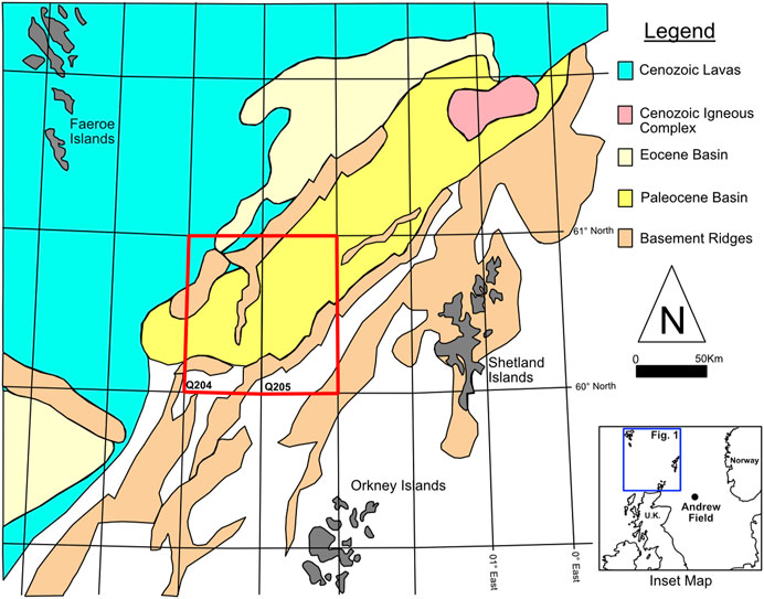
FIGURE 2. Geological map of Faroe-Shetland Basin after Freeman et al. (2008). The data used in this study is derived from boreholes in quadrants Q204 and Q205 (red box denotes location of Figure 1).
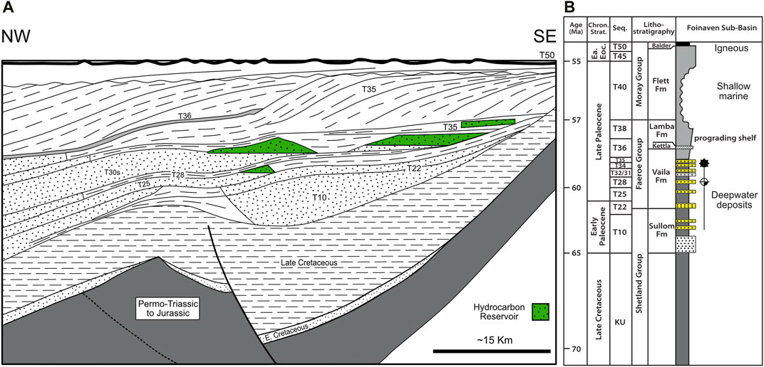
FIGURE 3. (A) Schematic cross section of the hydrocarbon reservoirs and surrounding strata. (B) Simplified stratigraphic column. Both figures modified from Lamers and Carmichael (1999) with additional information from Mudge (2015).
The Vaila Formation was deposited during the Paleocene, T22-T35 in the stratigraphic nomenclature developed by BP and Shell (Figure 3), and consists of deep-marine siliciclastic submarine fan deposits, with both sand-rich and mud-rich facies (Ebdon et al., 1995; Lamers and Carmichael, 1999; Leach et al., 1999; Ward, 2017). The Vaila Formation is equivalent to the Andrew Sandstone in the Lower Lista Formation in the North Sea (Leach et al., 1999, Mudge, 2015; Ward, 2017), a deep marine siliciclastic reservoir unit in the Cyrus and Andrew fields ∼600 km to the south east (Figure 2 inset). The interpreted depositional environment for the Vaila Formation in the study area is a submarine fan-channel system sourced from the south-southeast (Morton et al., 2002; Ward, 2017) (Figure 2). The hydrocarbons trapped in the Vaila reservoirs of Q204 are sourced from Kimmeridgian equivalent pre-rift Jurassic aged strata (Carr and Scotchman, 2003). Reservoir properties of the Vaila Formation are favorable, with porosity of ∼28% and horizontal permeability ranging from 500 to 1,500 milliDarcies (Richardson et al., 1997).
Our dataset consists of open-access core images and wireline logs from Quadrant 204 and 205, UKCS, collected during drilling activities for the conventional Foinaven, Alligin, Schiehallion, and Loyal fields (Figures 1, 2). All data are available online from the British Geological Survey. The study area was chosen because both well-log data and high quality color core images are available, and multiple wells with core from the Vaila Formation are located in close proximity to each other (Figure 1). Additionally, this dataset is ideal for image-processing and machine-learning workflow development, as the well-log data is high quality and has modern headers, and every core image was photographed under the same conditions (lighting, pixel dimensions, camera, and metadata) by the British Geological Survey (video, BGS, 2012). We specifically chose the British Geological Survey data because of this consistency, as many open-source datasets (e.g., Norway, New Zealand, United States Geological Survey, and various United States state repositories) have quite variable conditions of the core photographs, or no photographs at all.
We selected wells with at least 10 m of continuous core that was slabbed, photographed, and standard width (∼10 cm) (Table 1). We excluded intervals that were excessively broken or rubbly, impregnated or epoxied, had sample bags obscuring the core, or extensively sampled. Each image contains up to 3 m of core in a standardized tray (Figure 4) that includes a ruler, color calibration chart, and digital tablet screen showing meta-data (e.g., well name, box number, top and bottom core depth). Due to the consistent lighting over the whole dataset, no further editing or processing of the color spectrum was necessary to standardize the core-image dataset.
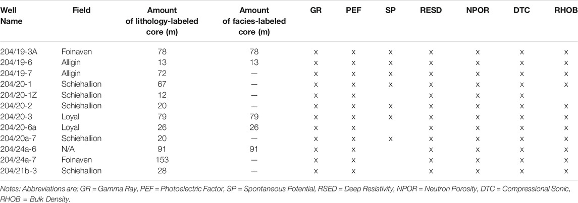
TABLE 1. Well-log and core dataset from Q204/205 used in this study. Amount of labeled core in meters.
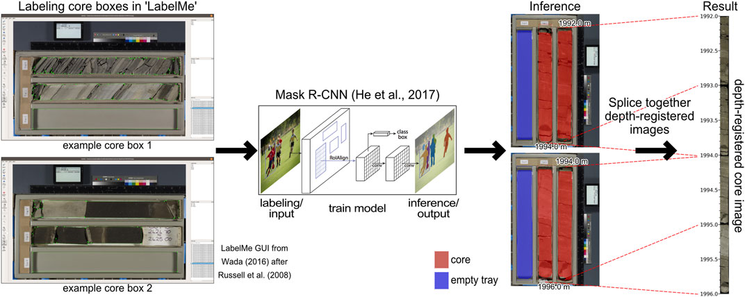
FIGURE 4. Workflow for creating depth-registered core columns (right) from a standard core photograph (left) using a machine-learning model. The workflow uses standard British Geological Survey hydrocarbon core images organized on a per-well basis and depth registration and creates ∼10 m long “core columns” that is only geologic material. These core columns are easily readable by machine-learning workflows. This core-image processing workflow requires some depth registering of each image and organization. Figure and workflow from Meyer et al. (2020).
The images utilized in this study are standard core tray photos from the British Geological Survey (BGS). The resolution for all the images in this study were consistent at 2,942 by 1,959 pixels for each photo of an entire BGS core tray (left side of Figure 4). The images were downloaded, converted from JP2 to JPEG format, and organized on a per-well basis. Each image was processed using the “corebreakout” methodology of Meyer et al. (2020) to obtain a “core column” image where each pixel is registered to the depth of the core (Figure 4). Meyer et al. (2020) use a machine-learning model to separate the core from the storage tray (non-geologic material) in an automated, reliable way. This method is more rapid and objective compared to manual methods that rely on cropping and aligning images one at a time using image-editing software. The productivity gain from using this automated workflow compared to manual methods speeds up editing by one to two orders of magnitude. We spot-checked core columns to ensure accuracy for both masking/cropping and depth registration; depth errors are <2 cm for any one core image, and the error is not additive for the core column.
Core columns at native resolution were generated and stored for each individual well in the dataset, with column images averaging roughly 600 pixels wide and ranging from ∼75,000 to 1,000,000 pixels in the depth dimension. We utilized rectangular patches method to segment the processed core column (Figure 5). Patches are 600 pixels wide and 32 pixels high, which is approximately 10 cm wide and 0.5 cm tall (Figure 5). Because training large neural networks for image classification is a memory-limited process, we use only the central 400 pixels of each row (Figure 5), and then further down-sample the images by a factor of two, resulting in image sections that are 200 pixels wide. This allows training examples to capture 6 times more vertical context than would otherwise be possible, and reduces total training time enough to make hyperparameter searches and training practical using consumer-grade hardware (10.5, Supplementary Materials). An additional benefit of using the central portion of the core (Figure 5) is that edge effects (e.g., cracks, core pieces with broken edges) are minimized.
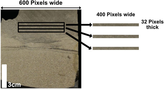
FIGURE 5. Diagram of image data and down sampling scheme. The full width core image is 600 pixels, and we downscale that to the central 400 pixels, and then further down sampled to 200 pixels. Each individual image feature is 32 pixels tall, scaling to ∼0.5 cm thickness in the core. Image from the 204-19-6 well at 2,215 m.
Because the image data are large and memory-intensive when modeling, we derived a “color-channel log”, a simple statistic that summarizes the brightness and color of the core image (Figure 6.). For each pixel row of the aligned core photographs, we computed the mean and variance of the red, green, blue, and greyscale pixel channels. These measurements depth registered make up the Color Channel Logs (CCL). This collapses the 400 pixels in each pixel row of the image to just eight values, reducing the volume of data by almost two orders of magnitude (Figure 6). This simple calculation creates a pseudo-lithology log directly from the images, where changes from sand to mud result in a shift in the log values (Figure 6). We experimented with using the greyscale log only, and found accuracy improvements using the red, green and blue color channels in addition to the gray. While some of this data may be redundant for some specific sections of core, this additional data did not significantly increase computational time. This method works with the Vaila Formation cores because 1) lithology is consistently linked to brightness and color, with sand typically white to light-tan, and mud being dark gray (Figure 6), and 2) the cores are generally cut perpendicular to bedding, so the lithologic contacts are generally horizontal and thus aligned with pixel rows. In cores with inconsistent lithology-color relationships and/or steeply dipping strata, this method would need to be modified to sum values along the bedding direction, or compute additional statistics that capture the heterogeneity across horizontal sections. As with the image data, the CCL is sensitive to poor quality images, shadows, and errors in masking. Dust, labels, or changes in lighting all will have a direct impact on CCL quality.
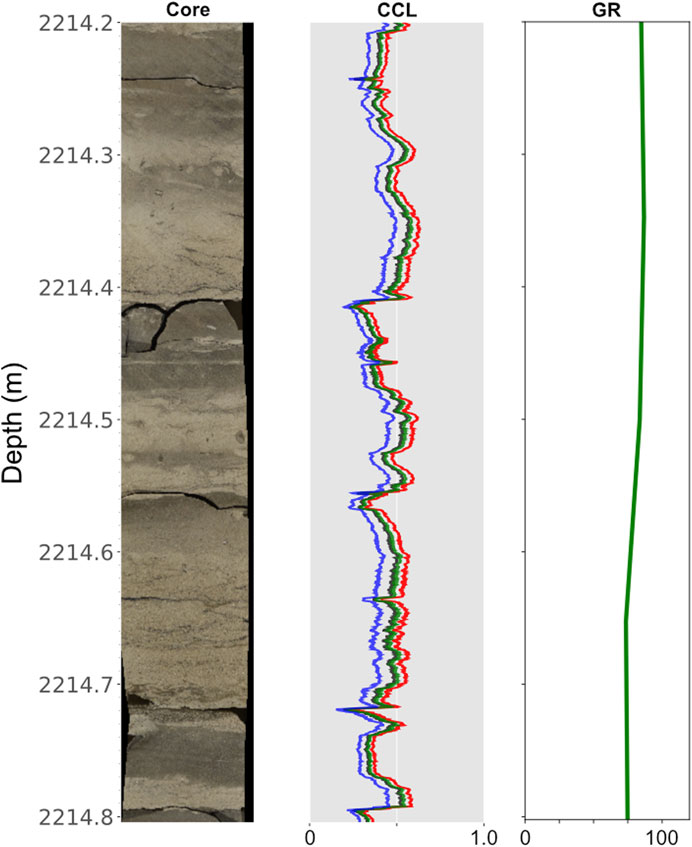
FIGURE 6. Example of core image (left), calculated color channel log(CCL, center) and gamma ray log (GR, right) from well 204/19-6 (depth in meters). We normalize the scale of the CCL log from 0–255 values to 0–1 on a per channel basis (i.e., red, green, blue and gray), representing the mean value for each channel across the core. Note that the CCL log captures fine-scale detail that the GR log does not. We evaluated only using the greyscale log and found improvement in accuracy using the red, green, blue, and gray logs.
Wireline log curves used in this study are open-source data files provided by the United Kingdom Oil and Gas Authority and include industry-standard tools (e.g., gamma-ray, resistivity, density, porosity; see complete log suites in Tables 1, 2). While many parameters can be determined or inferred from subsurface wireline measurements, standard log suites typically have vertical resolution ∼30–60 cm (Table 2). Modern image logs can have resolution of <1 cm (e.g., Rider and Kennedy, 2011), but such data were not available for this study.

TABLE 2. Resolution and use cases are from Rider and Kennedy (2011).
Well-logs were not edited or processed in any way to ensure reproducibility. For example, a depth shift is sometimes performed between core and wireline log data to align the two datasets (e.g., Fontana et al., 2010), but we chose not to depth-shift the wireline logs or core images in the study because 1) there is large subjectivity involved with the depth-shifting process, and 2) upon inspection of the two datasets, the logs and core are broadly depth-aligned, suggesting that any depth shift would be less than 0.3 m (about the vertical resolution of most well logs). We acknowledge that this may slightly degrade the performance of our comparisons between machine-learning models of log and core data, but creates a more simple, objective, and reproducible dataset.
A consistent and reliably labeled dataset is required for generating accurate inference using supervised ML methods (Sheng et al., 2008). Two different labeling schemes for the core data were created (Figure 7): 1) basic lithologies (e.g., sandstone, mudstone) and 2) a depositional-process-based sedimentary facies scheme (e.g., thin-bedded turbidites, hybrid event beds) similar to classification schemes employed by many core and outcrop-based turbidite studies (e.g., Lowe, 1982; Mutti and Normak, 1987; Sullivan et al., 2004; Hubbard et al., 2008; Bernhardt et al., 2011; Brooks et al., 2018). We labeled core at <2 cm resolution from the core images and use these labels for all of the data types (well-log, CCL, and image data). We acknowledge that subjectivity exists when labeling geologic material based on core photographs alone, and we attempted to be as consistent as possible; while we did not visit the BGS core repository, the photographs are very high resolution and allow for distinguishing texture and relative grain size (i.e., sand vs. mud). These labels provide a broad classification for defining lithological trends and depositional processes; the labels and machine-learning models are not designed and not able to interpret building blocks of these units, such as lamina, beds, and bedsets (sensuCampbell, 1967). For example, building a machine-learning model to identify ripple cross-lamination vs. parallel lamination would require a different, more focused labeling scheme. Lastly, it is best to have equal amounts of training data for each label when performing machine-learning inference (i.e., class (im)balance, Japkowicz, 2000). In order to honor the geologic complexity and the stratigraphic architecture of the dataset, class balance was not possible for this study (Figure 8). In other words, because of where the core was taken, there is more labeled thickness of mudstone than sandstone in the dataset (Figure 8). We use balanced class weighting during training, such that each class has an equal effect on the model regardless of prevalence in the dataset.
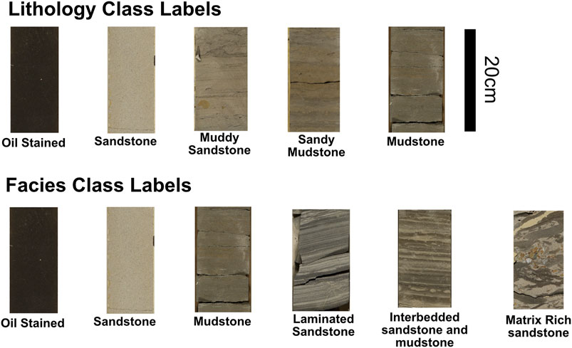
FIGURE 7. Example core images for lithology and facies labels. These labels were derived solely from core image interpretations.
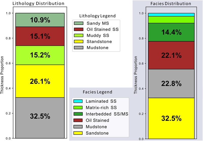
FIGURE 8. Distribution of thickness for lithology and facies in the overall, labeled dataset. Note the unbalanced classes for both lithology and facies studies. Laminated sandstone and Matrix-rich Sandstone classes for facies were 5.4 and 2.2%, respectively. Due to facies being a subset of the wells, the proportion of sandstone and mudstone are different compared to lithology.
We labeled 659 m of core from 12 wells with five basic lithologic labels: sandstone, muddy sandstone, sandy mudstone, oil-stained sandstone, and mudstone (Figure 7).
• Sandstone: sand grains comprise >95% of the lithology, with a <5% mud component, commonly as a muddy matrix or as mud clasts. Generally, sandstone is structureless (i.e., massive), but sometimes contains parallel or cross-laminated intervals. Color is bright tan to light brown.
• Muddy Sandstone: sand comprises 50–90% of the lithology, with 10–50% mud occurring as muddy matrix (Figure 7) or less commonly as interbeds. Sand beds commonly contain parallel- or cross-laminated intervals, and occasionally convolute lamination and mud clasts. Mud occurs as clearly defined interbeds or is incorporated into sand beds as swirly, lenticular intervals. Color is light to dark brown/gray.
• Sandy Mudstone: mud comprises 50–95% of the lithology, interbedded/interspersed with 5–50% sand. Sand beds commonly contain parallel- or cross-laminated intervals, and occasionally convolute lamination and mud clasts. Sand generally occurs as discrete beds, but some intervals are well-mixed, either due to depositional processes and/or bioturbation. Color is dark gray to brown.
• Oil-stained sandstone: Very similar to Sandstone (above) but stained by hydrocarbons. Sand grains comprise >95% of the lithology, with a <5% mud. Color is dark brown with interpreted inter-particle hydrocarbon residue.
• Mudstone: mud comprises >95% of the lithology, with a <5% sand occurring as discrete intervals <1 cm thick. We do not distinguish between silt and clay, rather lumping all sediment not distinguishable as sand into the mud component. Bioturbation is rare to occasional and dominated by Skolithos and/or Cruziana ichnofacies. Color is very dark gray.
This labeling scheme is designed to be widely applicable and objective and does not rely on any interpretation of depositional process, environment, water depth, or post-depositional diagenesis. A benefit of this lithologic labeling scheme is that it is applicable to many depositional environments (e.g., fluvial, shallow-marine, deep-marine). These five lithologic labels also very compatible with traditional petrophysical analysis (Passey, 2006). However, due to its simplicity, this scheme provides less information about sedimentary facies, sedimentary structures, and other characteristics useful for inferring depositional environment and dimensions of architectural elements (Cf. Mutti and Normark, 1987; Deptuck et al., 2008; Pettinga et al., 2018; Shumaker et al., 2018). We tested the number of lithology classes using unsupervized machine-learning techniques (e.g., k-means clustering) of the CCL data, and found that five classes is approaching the upper limit of appropriate number of clusters when comparing the silhouette scores. Thus, additional lithology classes probably would not improve the research result for this dataset, but in fact may degrade the results.
We also labeled 287 m of core data from five wells (Table 1) using the following depositional-process-based facies scheme: structureless sandstone, laminated sandstone, matrix-rich sandstone, interbedded sandstone/mudstone, mudstone, and oil-stained rock (Figure 7). These facies are briefly described below, and the structureless sandstone, mudstone, and oil-stained rock are identical to the lithology labeling scheme. We identified these facies from visual patterns, color, texture, and relative scale. These facies capture the most common types of heterogeneity observed in this dataset and provide more contextual geologic information than lithology. The labels were interpreted to the core (<1 cm) scale. Sedimentary structures and event-beds documented in the core are consistent with a deep-marine interpretation and include low- and high-density turbidites (Bouma, 1962; Lowe, 1982) as well as hybrid event beds (sensu Haughton et al., 2009). The facies in our study area are quite similar in style and interpreted process to those described by Bouma (1962), Lowe (1982), Lowe and Guy (2000), Haughton et al., (2009), and summarized by Talling et al. (2012).
Sandstone, Mudstone, and Oil-stained sandstone are identical to the lithology labels, and their descriptions can be found above. The sandstone and oil-stained sandstone facies are interpreted to be high-density turbidity current deposits (sensuLowe, 1982). The mudstone facies is interpreted to be low-density turbidity-current and hemipelagic deposits, although we did not distinguish between these two deposit types in our labeling scheme.
Matrix-rich sandstone consists of light-to dark-colored sandstone, commonly with swirly textures, shear fabrics, mud clasts, and sand-injections. These deposits are interpreted to be deposited by “hybrid” sediment gravity flows (i.e., those with transitional flow rheologies). These “hybrid event beds” (also referred to as slurry beds, linked debrites, and several other textural terms) have been extensively described in the subsurface of the North Sea (e.g., Lowe and Martin, 2000; Barker et al., 2008; Haughton et al., 2009) and in many other outcropping and subsurface submarine depositional systems (see review in Talling, 2013). The hybrid event beds of the Vaila Formation often contain a disorganized, swirly texture of both sand and mud at varying scales (0–5 cm in core, Figure 7) as well as mud clasts, similar to textures reported in other hybrid-event-bed studies (e.g., Lowe and Martin, 2000; Haughton et al., 2009; Pierce et al., 2018). Individual mud clasts can vary from a few millimeters to the width of the core (∼10 cm), are rounded, and vary from circular to lenticular in shape.
Laminated sandstone consists of fine-scale (<0.2 cm) alternating dark and light colored laminae and likely represents the upper-flow regime, parallel-laminated Tb division of a Bouma sequence (Bouma, 1962). The dark colored bands are interpreted to be heavy-mineral rich, as they do not appear to be mud rich due to their color and stacking pattern. However, we did not visually inspect these cores as we only had access to the photos and cannot unequivocally say there is no mudstone present in these laminated sandstone deposits.
Interbedded sandstone and mudstone consists of stacked ∼1 cm thick sandstone beds and mudstone intervals (i.e., heterolithic bedding). These deposits are interpreted to be “thin-bedded turbidites,” the deposits of low-density turbidites in an off-axis environment. While we interpret a general off-axis environment, these deposits can occur in levees (Hansen et al., 2017) and other channel-overbank environments (e.g., Jobe et al., 2017), as well as both proximal, lateral, and distal submarine-fan settings (Spychala et al., 2017). Without further context from seismic or other data, we do not speculate on the particular environment.
All code and data from this study are available on the github repository, https://github.com/rgmyr/coremdlr (Meyer and Martin, 2021). The installation guide, Jupyter Notebooks (Kluyver et al., 2016), processing routines, and installation instructions are included in the repository. The requirements for installation are:
Python 3.x.
Numpy (Harris et al., 2020).
Scipy (Virtanen et al., 2020).
Matplotlib.
Scikit-image.
Scikit-learn.
Tensorflow.keras.
These dependencies are all maintained and open source.
We experimented with various supervised machine-learning models, and chose the models described below based on performance, usability, and flexibility for each data type. Each model is open-source, currently maintained, and is used natively in Python. The code, parameters, and specific models used to produce the results in the study are included in the supplementary materials. The choice for each data type to have its own model was driven by data structure and density (e.g. well-logs vs. images). We evaluated combining these datasets but the complexity in implementing this into the model construction proved to be unwieldy and ultimately did not improve performance.
Because the stratigraphic record is built on the principle of superposition, information both above and below a region of interest is important for understanding the evolution of stratigraphic architecture. We utilize a thickness-based, sliding-window approach for both training and inference. This ensures that the model incorporates context both above and below every labeled interval during training. This approach also makes inference less sensitive to missing context at window boundaries, as predictions are averaged wherever two adjacent windows overlap. For a particular labeled target interval, the model incorporates weights both above and below the window at each thickness step (24–64 cm for image and CCL data, respectively). This method is also commonly used for machine-learning analysis of time series data (Ma and Hovy, 2016; Zeng et al., 2016).
Four metrics are used to score the overall performance of each model with associated training and testing data set: Accuracy, Precision, Recall, and F1, all of which are defined in Eqs 1–4, respectively. Accuracy is an important and commonly used metric, but does not capture the variability of performance in an unbalanced dataset (i.e., not the same number of labels for each class–also see Figure 8). Precision and recall better assess the class imbalance of the training and testing data, and F1 is a combined metric of precision and recall. Each metric for each dataset will be released in the Supplementary Materials (Supp. Mat. 10.3), but we will focus on Accuracy and F1 below (Figure 9).
where Tp is true positive predictions, Tn is true negative, Fp is false positives and Fn is false negatives. (also see Figure 9).
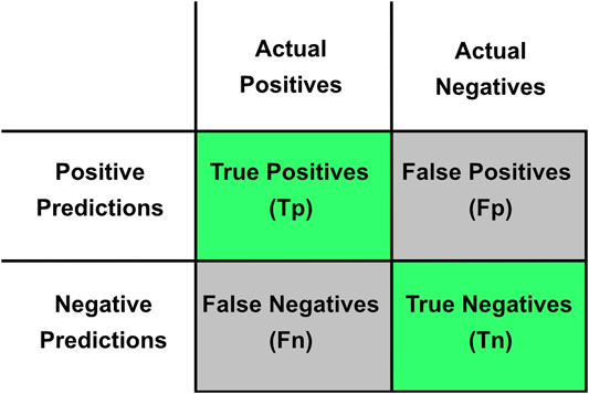
FIGURE 9. Confusion matrix of True Positives, False Positives, False Negatives, and True Negatives. Green shading represents correct predictions, and gray shading represents incorrect predictions.
Supervised machine-learning models generally train on a subset of an entire dataset, and then perform inference (i.e., test) on a different subset. This eliminates using training data on the testing data, which can lead to overfitting. Our lithology dataset consists of twelve wells (Table 1), and so we divided the wells into training sets that consist of three, six, and nine wells (10.4, Supplementary Materials). We determined that five test-train runs for each set was enough to capture heterogeneity in the training data, while being tractable to run. We grouped training sets by creating a mix of different wells in each set; no two sets are the same. We chose this method for reproducibility rather than randomly assigning wells to train-test splits. For facies labels, only five wells have labels, so each single test well was trained by the rest of the wells in the dataset (see Table 1); therefore, testing and training was done five separate times, with different training and testing wells in each run.
We chose these methodologies for lithology and facies labels as it emulates a traditional geoscience interpretation workflow; a geoscientist typically interprets all the core data from one well for a subsurface interpretation and then compares it against other nearby wells. Splitting on a per-well basis also avoids data leaking between testing and training datasets. We feel that this honors the data and traditional geoscience workflows better than a typical ML workflow, which would randomly assign test and train splits or use weighting to achieve a balanced label proportion for each test-train split. Geoscience based ML contests typically utilize the strategy of test-train splitting on a per-well basis to avoid overfitting (e.g., Hall and Hall, 2017).
XGBoost (Chen and Guestrin, 2016) is an open-source gradient boosting library. Gradient boosting is an algorithm for building a strong ensemble model by combining many weak base predictors, usually decision trees (Quinlan, 1986). Trees are added to the ensemble sequentially, with later trees constructed to minimize the error from earlier trees, subject to regularization constraints that help prevent overfitting. XGBoost was used to build the winning model in the Higgs Boson Machine Learning challenge and is used widely for various machine-learning applications (e.g., Chen and He, 2014). Gradient boosted tree models easily accommodate missing values and non-standard data types, are indifferent to the scale or normalization of input features, and their performance is relatively insensitive to hyperparameter settings (especially compared to neural networks). These properties make them useful and convenient as a baseline for relatively incomplete data types, like well-log data, where not every well has the same suite of downhole measurements (e.g., Table 1).
In our study, XGBoost was used to train models for predicting lithology and facies from well-log data. The labels for the well-log data were derived from the core images, as described above. These labels, ∼0.5 cm in thickness, were mapped onto the depth values for the well-log data using linear interpolation from typical well-log resolution, which ranges from 15 to 60 cm (Table 2).
WaveNet (Oord et al., 2016) is a convolutional neural network (CNN) model architecture that was originally designed as a generative model for raw audio waveforms, with applications in text-to-speech, music generation, and speech recognition. The blocks that comprise the network consist of stacks of dilated convolutions, which perform multi-scale context aggregation (Yu and Koltun, 2016), coupled with causal filters (Oord et al., 2016) that prevent “current” output from using “future” information, assuming the input and output sequences are time domain equivalent. Because we want stratigraphic context both above and below the “current” output, we modified the original WaveNet architecture to perform variable-resolution sequence-to-sequence learning (Sutskever et al., 2014) and removed the causal filters to allow the model to use context both above and below the individual prediction targets. This is broadly analogous to how a geoscientist interprets stratigraphic data, taking into account information from the strata and stacking patterns both above and below an interval to make a context-dependent prediction. We also experimented with recurrent neural network (RNN) architectures but found that they did not improve performance and were less stable during training (Bai et al., 2018).
It's not necessary to apply additional transformations to the CCL data because CNNs (and in general, deep neural networks with non-linear activation between layers) can learn to approximate any of those functions. The only reason to apply a transformation to input features is to make them more normally distributed, and even then this generally only improves convergence time rather than improving the model.
Compared to XGBoost, the WaveNet CNN model requires more standardized data input. WaveNet models were trained and tested on the CCL log data (Figure 6), and models were configured so each 32 pixel section of a CCL log is mapped to a single ∼0.5 cm (32 pixel height) prediction. Because the CCL data is 50x smaller in size than the image data for a given depth interval, this efficiency allows for larger vertical extents of perception (i.e., window size) using CCL data compared to image data.
Classification of geological images aligns well with the problems in image processing known as texture recognition, texture classification, or fine-grained image classification (grain in this case referring to classification of subtly different objects e.g., different models of cars, not geologic grains). These terms broadly refer to the modeling of image datasets where the salient differences between images are small, repeated patterns and local image statistics, rather than more global geometric structures and their relative positions and orientations (Wei et al., 2019).
Deep TEN (Zhang et al., 2020) is a Convolutional Neural Network (CNN) model architecture that adapts dictionary learning, a popular and successful approach to image texture classification (Liu et al., 2019), as a trainable component of the neural network. We adapted the network to take depth-aligned core images as input (see Figure 5), and predict sequences of labels as output (rather than a single classification per image) (Figure 7). As with WaveNet, this allows the network to consider context above and below the individual labels when making predictions–however, the sequences could not be as long, since image data is two orders of magnitude larger memory size than CCL per unit depth. Other researchers have used CNN models on carbonate core image data with success (Pires de Lima et al., 2019).
To further emphasize contextual information for predictions, we also added recurrent neural network layers (Long Short-Term Memory, Gated Recurrent Unit) to the feature sequences generated by Deep TEN (Shi et al., 2015) but ultimately this increased training overhead without any appreciable improvement in performance.
Figure 10 shows the difference between two metrics for all of the lithology experiments. The well-log data models had a maximum accuracy of 35.7% (nine training wells) and minimum accuracy of 18.2% (six training wells). None of the metrics improve significantly with more training data for well log data. For perspective on this accuracy, a randomly generated model would have an accuracy roughly equivalent to the proportion of the most common class (mudstone = 32.5%, Figure 8), the well-log data predictive performance is similar to randomly choosing a class.
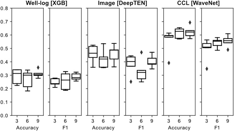
FIGURE 10. Box plot of Accuracy, Weighted F1 for lithology prediction on all data types. X axis is number of training wells (3, 6, and 9). A perfect score would be a score of 1.0, but because there are five classes, a 0.2 score represents random-choice, while a 0.5 score is significantly better than random. Typical baseline for ML models is if you predicted the most common class, which in this case predicting all Mudstone would result in an accuracy of 0.325. The well-log data used XGBoost ML model, Image used Deep TEN and Color Channel Log (CCL) used WaveNet respectively.
The image data models had a maximum accuracy of 57% (six training wells) and minimum accuracy 36% (six training wells), respectively. This data type is less accurate and has longer compute time compared to CCL data. Additional training data did not improve performance for this data type. Models using CCL data had a maximum accuracy of 69% (nine training wells) and minimum accuracy of 39% (three training wells), respectively. The maximum accuracy for six training wells is 65%.
The WaveNet model using CCL data was the fastest to compute and had the most accurate results; it was the only data type to show improvement with more training data. As shown in Figure 10, the most accurate model run for each test and train set did not improve substantially using CCL data, but the outlier of 39% on the three well test and train set was avoided using six wells. The intermediate lithologies have an irregular and heterogeneous CCL signature, compared to the more continuous sandstone and mudstone character (Figure 11). Along with character, these signatures also vary in magnitude, and the end-member lithologies (sandstone, mudstone) are clearly separated, whereas the intermediate lithologies can have overlapping CCL values. In Figure 11, 2215.3–2215.8 m results demonstrate the power of this workflow. Both models capture the correct sandstone thickness and the sharp transition to mudstone above and below it.
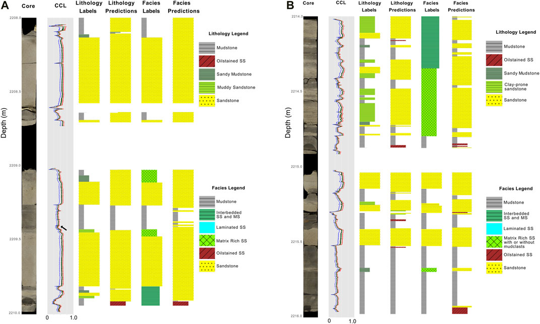
FIGURE 11. Example of core image, CCL, lithology and facies labels and predictions for one well, 204-19-6. Part A ranges from 2,008 to 2,010 m and part B ranges from 2,214 to 2,216 m measured well depth below sea surface. These model results are from nine training wells using the CCL data to predict both lithology and facies.
The WaveNet model generally predicts homogeneous sandstone and mudstone well (Figures 10, 11), but intermediate lithologies are not predicted to the same accuracy. The stacking patterns of typical turbidites are preserved in the CCL data (e.g., fining upward turbidites, Figure 11), but bed boundaries aren’t always predicted accurately. However, the overall sand-mud ratio is generally preserved, even for misclassified sections (e.g., 2209.4 m in Figure 11); the changes in CCL character are correlated to the interpreted lithology in this section (Figure 11), but the model over-predicted the amount of sandstone.
Figure 11 demonstrates how the WaveNet model predicted facies from CCL data. For example, the very thin sand bed at 2,209.3 m was predicted correctly by the model even though it was not labeled as a sandstone facies. However, the interval 2214.0–2214.4 m in Figure 11 has a facies label of “interbedded sandstone and mudstone” but the model predicts thinner, stacked “sandstone” and “mudstone” facies labels. In this case, the model predictions are incorrect, but may be acceptable for some geologic workflows (e.g., net-to-gross determination over a large area). However, in some cases, the model predictions are more “correct” than the labeled “truth” (e.g., 2214.2 m in Figure 11) this could be especially helpful if this workflow is used to assist/bolster manual core description. Hence, judging model accuracy and utility in these situations is difficult, and creating a metric that captures this ambiguity in “geologic reasonableness” is difficult to implement for ML models.
A confusion matrix (Figure 12) provides insight into misclassification for each labeled class; an ideal model would only have values in the diagonally aligned boxes that define true positive (Tp) predictions (also see Figure 8). In our model, Sandstone and Mudstone had the best predictions (Figure 12) while Muddy Sandstone and Sandy Mudstone had the least accurate predictions. These two intermediate lithologies were more commonly predicted as mudstone and Oil Stained Sandstone, but also were sometimes interpreted as Sandstone. While the exact lithology label is sometimes predicted incorrectly, the boundaries of individual sedimentation units (i.e., beds) and their thicknesses are generally preserved (Figure 11). Merging the two intermediate lithology classes would improve model accuracy but would somewhat limit the utility of the predictions (e.g., for detailed petrophysical or geological work).
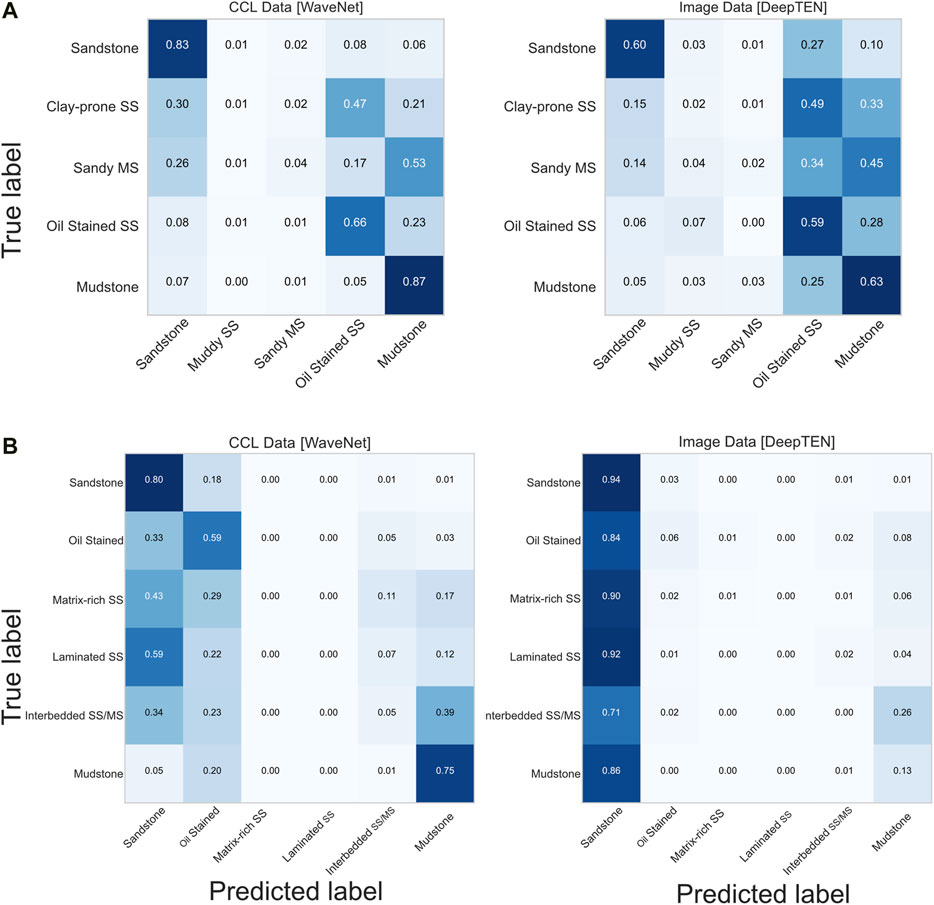
FIGURE 12. Part (A) Confusion matrices from the nine well test sets for both CCL and Image model runs. The matrices are overall performance, and include all five sets for each group. A perfect model would only have predictions on the diagonal, and a score of 1.0 (i.e., 100%) within a box. The majority of misclassification was an intermediate lithology predicted as oil stained or as mudstone. The maximum accuracy of an intermediate lithology was 0.04 (4%) for sandy mudstone using CCL. Part (B) Confusion Matrices from CCL data (left) and image data (right) for the six facies categories. A perfect score would be 1.0 for an individual box, in the diagonal.
Facies testing with five of the twelve wells had limited success with accurately predicting the three newly introduced facies labels. For example, only 5% of interbedded sandstone and mudstone was predicted correctly (Figure 12), with this facies much more commonly misclassified as Sandstone or Mudstone (see discussion above and 2214.2 m interval in Figure 11). For interbedded sandstone and mudstone, label vs. prediction thickness is potentially an issue for prediction accuracy, as strict definitions for class labels must be determined when labeling a layer as interbedded sandstone and mudstone compared to individual layers of sandstone and mudstone. These thickness parameters and cutoffs are an interpretation that has impact on modeling, accuracy, and training.
Mudstone predictions are very good using the lithology labels (63% image-data and 87% CCL-data accuracy, Figure 12) and the facies-labels with the CCL models (75%, Figure 12). However, mudstone predictions using the image-data and facies labels has only 13% accuracy (Figure 12). The misclassification of the mudstone facies using the image data may be attributed to 1) more limited training data compared to the lithology data set (Figure 8), or 2) more complex class labels compared to the lithology dataset. This can be problematic for neural net class of models. Increasing training data of these more uncommon classes and the overall size of the dataset can only help prediction of these facies. At this level of prediction performance, data is the limiting factor, not ML model choice. Increasing computing power for the image data would not necessitate as much down sampling and loss of finer scale details. This combined with limited sequence length might be one reason for poor performance.
The more complex facies (e.g., laminated sandstone) performed similarly to the intermediate lithology classes for prediction with the CCL data. The facies classes (Figure 7) compared to the lithology endmembers (Figures 7, 11) can have similar CCL log characteristics to each other and these lithology end members. The CCL data alone does not capture all of the heterogeneity or detail of the native core image interpretations, and subtle differences become more nuanced with this data type and complex class labels.
The greater amount of information in the image data did not improve performance compared with CCL data. In fact, our results demonstrate that CCL data are more accurate than image data and require fewer computing resources for the same amount of data. By calculating the CCL curves, we may be filtering out less important geologic features or small-scale heterogeneities that are unimportant for prediction but create noise in the image data. One factor that might hamper the accuracy of the image data is the thickness of the image slices; 32 pixels (0.5 cm) might not be thick enough to provide proper context for correct prediction. However, experimenting with enlarging the thickness window size to 64, 128 and larger pixels did not improve performance. In fact, performance was degraded in most cases, at least partially due to the fact that with thicker label sizes, multiple classes were agglomerated into one label, reducing the total amount of training data available. Training data for this project was created as true to core scale as possible with no thought to minimum size of each interpretation, so some labels are only 0.5 cm or 1 cm thick. Future work could explore segmentation of the core based on clustering or other parameters (e.g., Luthi, 1994), then predict on that segmented core with various label scales instead of pre-defined bin sizes (e.g., 1 cm); with larger label size/thickness, a minimum threshold of label size could potentially improve model performance, but at the cost of high-resolution detail.
The lack of accuracy for facies for both CCL and Image data could be caused by the scale of the labels (as just discussed), or perhaps a lack of training data (Figure 8). Increasing the number of facies labels with the current amount of training material would not improve model performance for image or CCL data types. Accurate prediction of facies will probably require larger and more strictly defined labels and datasets other than the one explored in this research. The model for predicting facies from image data (Deep TEN) was chosen from testing on lithology, but potentially more complex visual characteristics of facies (e.g., laminated sandstone, mud clasts) will require different machine-learning models. As geological parameters from images becomes a more standard workflow, more research will focus on what texture-based ML models perform best (Adebayo et al., 2018).
Well-log data did not perform at an accuracy level that would be useful for typical standard core-based geoscience workflows. In fact, the best performing models would have had similar accuracy by just predicting mudstone (Figure 8). Thus, predicting core level (<1 cm) detail is not possible with current standard well-log data, which is perhaps not a surprising result considering typical well-log resolution (Table 2). Adding micro-resistivity, image log, or other higher resolution downhole tools may vastly improve the prediction at the core (<1 cm) level. Previous studies that use standard well-log information on core-derived classes (Hall and Hall, 2017) have label intervals that are closer to well-log scale at ∼15 cm thickness, roughly thirty times larger than our label resolution. Label size for all data types is an important parameter that will affect the amount of labeling, algorithm choice, and model architecture. Relabeling a dataset manually is labor intensive, and thus picking an appropriate scale for labels is an important task that has many downstream effects on the modeling results.
To improve on this result using similar core quality and deposit type, additional digital data types could be used. Hyperspectral imaging or multispectral imaging of slabbed core, computed tomography (CT) scanning, micro-XRF, and downhole image logs are a few examples of data types that could be utilized to provide more information into mineralogical, chemical, or physical properties of the core. However, these involve additional costs and considerations compared to standard photographs and are often not available for legacy datasets that are stored in core warehouses around the world. Conveniently, our current workflow is expandable to these types of digital depth-registered datasets with minimal modifications necessary.
The results for nine training wells of CCL data types with five lithologies indicate an overall accuracy of 62% for all sets, with the best set reaching 69%. The Sandstone and Mudstone classes are predicted even more accurately (>80%). Model prediction of just Sandstone for the entire well would result in an accuracy of 32.5%. Using these machine-learning models improves this result by roughly 200%. Our workflow is capable of producing accurate lithology predictions for thousands of meters of core relatively quickly (100s of meters in minutes) using current standard consumer computer hardware (10.5, Supplementary Materials). The two intermediate lithology labels are the most challenging to predict. Additionally, because intermediate lithologies are less common in this dataset (Figure 8), a lack of training data further inhibits the prediction.
This workflow will be very useful for basin-scale studies of a specific formation (e.g., net-sand-thickness map from core data) or for applications where a practitioner could conduct initial screening to highlight wells with lithologies of interest. This technique is of particular value in cases where logging/describing individual cores is not feasible due to the volume of core to process or core that isn’t available for in-person examination. An example of this would be core from a data trade, or examining entire databases, such as the USGS Core Research Center (Hicks and Adrian, 2009).
However, the accuracy produced by this study is not capable of replacing core descriptions performed by trained geoscientists, nor is it meant to - this study attempts to encompass the full range of deep-marine depositional variability in five lithologies and six lithofacies. However, k-means clustering indicates that increasing the number of classes without accompanying increases in training data is not advised with this dataset. The five labeled lithologies are broad, and provide no insight into grain size, sedimentary structures, depositional process, bioturbation, chemical composition (such as cementation or mineralogy), or diagenesis. We attempted to reproduce some of this detail using the facies labeling scheme, with unsatisfactory results. Perhaps these more detailed features could be labeled and predicted using ML methods (e.g., Tang et al., 2020), but investigating these more detailed labeling schemes and their accuracy is outside of the scope of this study. Geologic class labels with subtle and nuanced differences and features (e.g., lithofacies, ichnofacies) will need specific and consistent labeling definitions to be successful.
Furthermore, while we labeled each class as consistently and accurately as possible, it is possible that errors exist in our labels (Northcutt et al., 2021) or that our label selection was biased by previous training, experience, and uncertainty (Cf. Bond et al., 2007). Because label selection is inherently qualitative and scale-dependent, we did not incorporate any uncertainty metric into our labeling scheme. Each label was considered the absolute correct answer in this study, and if the label is incorrect it will affect the accuracy of the resulting inference. Future work could develop a method for assigning uncertainty to labeled geologic data and propagate that error into the modeling workflow, including assessing when the model gives an incorrect prediction but still accurately portrays the lithology or scale of the core. Finally, we hope that this study can serve as a baseline for future work to improve labeling schemes and/or ML model selection/methodologies.
This study utilized only 1D, borehole-based data types. One way to extend the prediction capability is by incorporating spatial information and metrics. For example, utilizing forward stratigraphic models to generate stratal surfaces, geometries, and scales could be incorporated into spatial prediction of lithology and facies (Mulder et al., 1997; Tinterri et al., 2003; Pyrcz et al., 2005; McHargue et al., 2011; Albertão and Athayde, 2015; Burgess et al., 2019; Zhang et al., 2020). The model results might also provide another metric to score the results from machine-learning outputs. Other empirical data that focuses on spatial lithology heterogeneity (e.g., bed thinning rates derived from outcrops, Fryer and Jobe, 2019) could be utilized to provide possible inter-well lithology predictions and correlations. This hybrid approach of using forward-modeling results and empirical data to guide machine-learning predictions is a clear direction to advance geoscience-focused machine learning workflows. Other data that could be incorporated include routine core analysis from plugs and/or thin sections (e.g., Anselmetti et al., 1998; Tang et al., 2020).
Expanding this workflow into other rock types (carbonates, igneous, metamorphic) could change which workflow or data type performs the best. As demonstrated by our research, the quantity of training data needed to train a model with usable results can be as few as six wells worth of core, each with 10–100 + m of core (Cf. Table 1). Labeling hundreds of different wells might be necessary if trying to capture a wide range of lithologies and depositional environments (or very specific structures, e.g., ripples), but less high-quality training data may be needed if the project is limited to a specific depositional environment. Fluvial, shallow-marine, and other predominantly siliciclastic deposit types would be a natural extension of this workflow, and open-access core exists that could be labeled. However, for carbonate and evaporite rocks, we suggest incorporating additional data types as suggested above (e.g., hyperspectral image data) that can better detect differences in physical and chemical properties.
This study utilizes open-source borehole data from Quadrant 204 on the United Kingdom Continental Shelf to evaluate the utility of automated lithology prediction. 659 m of core from 12 wells were labeled at the sub-centimeter scale, utilizing a lithology-based labeling scheme (five classes) and a depositional-process-based facies labeling scheme (six classes). The best-performing models utilize a “color-channel-log” (CCL) that summarizes the image at each depth interval, with model accuracy >80% for Sandstone and Mudstone lithology classes, and an overall accuracy of 69% for five lithology classes for the best performing model. Furthermore, the CCL data was the faster to compute and had the most accurate results, likely because the CCL data summarizes data important for lithology prediction.
While facies-based labels are important for characterizing depositional processes and environments, model prediction is not as accurate as more strictly defined lithology labels. This poor performance is likely caused by lumping of multiple lithologies into one label (e.g., interbedded sandstone-mudstone). Well-log data did not perform at an accuracy level that would be useful for typical standard core-based centimeter-scale (<5 cm) geoscience workflows.
This study demonstrates the potential to transform hundreds of thousands of meters of previously photographed core into a normalized and digital format with specific geological insight and interpretations using standard consumer desktop hardware and open-source data and software. The workflow is also general enough for any basin-wide or other large scale subsurface investigation that requires lithology identification; thus, any geoscientist interested in assimilating large subsurface datasets can utilize these techniques for better characterizing core-image data for applications in mining, hydrogeology, geothermal, carbon sequestration, and geotechnical studies. Machine-learning workflows will not replace the need for geoscientists’ interpretations, but they can augment and speed up specific repetitive tasks (e.g., core description), especially when applied at the broad, basin scale. Interpretation of core images alone will never replace physical inspection of the core material by an experienced geoscientist.
The original contributions presented in the study are included in the article/Supplementary Material, further inquiries can be directed to the corresponding author.
All authors contributed to conceptualization of the project, figure generation, and writing the manuscript. TM labeled all core images, compiled geologic background, and analyzed results. RM developed and executed the models and workflows. ZJ developed the color-channel-log method and assisted with facies and lithology class selection.
Funding was provided by Chevron through Chevron Center of Research Excellence at Colorado School of Mines (core.mines.edu).
The authors declare that the research was conducted in the absence of any commercial or financial relationships that could be construed as a potential conflict of interest.
The handling editor declared a past co-authorship with one of the authors (ZJ).
We acknowledge the funding support from Chevron Center of Research Excellence (core.mines.edu) at Colorado School of Mines. Fruitful discussions and research ideas were generated and refined on the software underground (https://softwareunderground.org). We thank associate editor Anne Bernhardt and three reviewers for providing reviews that significantly improved the results and readability of the manuscript.
Adebayo, J., Gilmer, J., Muelly, M., Goodfellow, L., Hardt, M., and Kim, B. (2018). Sanity Checks for Saliency Maps. Advances in Neural Information Processing Systems 2018-Decem(NeurIPS), 9505–9515.
Albertão, G. A., Mulder, R. T., Teles, V., Chauveau, B., and Joseph, P. (2015). Modeling the Deposition of Turbidite Systems with Cellular Automata Numerical Simulations: A Case Study in the Brazilian Offshore. Mar. Pet. Geology 59, 166–186. doi:10.1016/j.marpetgeo.2014.07.010
Anselmetti, F. S., Luthi, S., and Eberli, G. P. (1998). Quantitative Characterization of Carbonate Pore Systems by Digital Image Analysis. AAPG Bull. 82 (10), 1815–1836.
Bai, S., Kolter, J. Z., and Koltun, V. (2018). An Empirical Evaluation of Generic Convolutional and Recurrent Networks for Sequence Modeling. Available at: http://arxiv.org/abs/1803.01271.
Baldwin, J., Bateman, R., and Wheatly, C. (1990). Application of a Neural Network to the Problem of Mineral Identification from Well Logs. Petrophysics 31 (5), 279–293.
Barker, S. P., Haughton, P. D. W., McCaffrey, W. D., Archer, S. G., and Hakes, B. (2008). Development of Rheological Heterogeneity in Clay-Rich High-Density Turbidity Currents: Aptian Britannia Sandstone Member, UK Continental Shelf. J. Sedimennt. Res. 78, 45–68. doi:10.2110/jsr.2008.014
Bernhardt, A., Jobe, Z. R., and Lowe, D. R. (2011). Stratigraphic Evolution of a Submarine Channel-Lobe Complex System in a Narrow Fairway within the Magallanes Foreland Basin, Cerro Toro Formation, Southern Chile. Mar. Pet. Geology 28 (3), 785–806. doi:10.1016/j.marpetgeo.2010.05.013
Bond, C. E., Gibbs, A. D., Shipton, Z. K., and Jones, S. (2007). What Do You Think This Is? "Conceptual Uncertainty" in Geoscience Interpretation. GSA Today 17 (11), 4–10. doi:10.1130/gsat01711a.1
Bouma, A. H. (1962). Sedimentology of Some Flysch Deposits: A Graphic Approach to Facies Interpretation. Elsevier, 168 p.
Brooks, H. L., Hodgson, D. M., Brunt, R. L., Peakall, J., Hofstra, M., and Flint, S. S. (2018). Deep-Water Channel-Lobe Transition Zone Dynamics: Processes and Depositional Architecture, an Example from the Karoo Basin, South Africa. Bull. Geol. Soc. America 130 (9–10), 1723–1746. doi:10.1130/b31714.1
Burgess, P. M., Masiero, I., Toby, S. C., and Duller., R. A. (2019). A Big Fan of Signals? Exploring Autogenic and Allogenic Process and Product in a Numerical Stratigraphic Forward Model of Submarine-Fan Development. J. Sediment. Res. 89 (1), 1–12. doi:10.2110/jsr.2019.3
Campbell, C. V. (1967). Lamina, Laminaset, Bed and Bedset. Sedimentology 8 (1), 7–26. doi:10.1111/j.1365-3091.1967.tb01301.x
Carr, A. D., and Scotchman, I. C.(2003). Thermal History Modelling in the Southern Faroe–Shetland Basin. Pet. Geosci. 9 (4), 333–345. doi:10.1144/1354-079302-494
Chen, T., and Guestrin, C. (2016). Xgboost: A Scalable Tree Boosting System. Proceedings of the 22nd Acm Sigkdd International Conference on Knowledge Discovery and Data Mining, San Francsco, CA, USA, August 13–17, 2016, KDD ’16, 785–794. doi:10.1145/2939672.2939785
Deptuck, M. E., Piper, D. J. W., Savoye, B., and Gervais, A. (2008). Dimensions and Architecture of Late Pleistocene Submarine Lobes off the Northern Margin of East Corsica. Sedimentology 55 (4), 869–898. doi:10.1111/j.1365-3091.2007.00926.x
Dramsch, J. S. (2020). 70 Years of Machine Learning in Geoscience in Review. Adv. Geophys. 61, 1–55. doi:10.1016/bs.agph.2020.08.002
Dunham, M. W., Malcolm, A., and Kim Welford, J. (2020). Improved Well-Log Classification Using Semisupervised Label Propagation and Self-Training, with Comparisons to Popular Supervised Algorithms. Geophysics 85 (1). doi:10.1190/geo2019-0238.1O1–O15.
Ebdon, C. C., Granger, P. J., Johnson, H. D., and Evans, A. M. (1995). Early Tertiary Evolution and Sequence Stratigraphy of the Faeroe-Shetland Basin: Implications for Hydrocarbon Prospectivity. Geol. Soc. Spec. Publ. 90 (90), 51–69. doi:10.1144/gsl.sp.1995.090.01.03
Ellis, D., and Stoker, M. S. (2014). The Faroe-Shetland Basin: A Regional Perspective from the Paleocene to the Present Day and its Relationship to the Opening of the North Atlantic Ocean. Geol. Soc. Lond. Spec. Publications 397 (1), 11–31. doi:10.1144/sp397.1
Fontana, E., Iturrino, G. J., and Tartarotti, P. (2010). Depth-Shifting and Orientation of Core Data Using a Core-Log Integration Approach: A Case Study from ODP-IODP Hole 1256D. Tectonophysics 494 (1–2), 85–100. doi:10.1016/j.tecto.2010.09.006
Freeman, P., Kelly, S., Macdonald, C., Millington, J., and Tothill, M. (2008). The Schiehallion Field: Lessons Learned Modelling a Complex Deepwater Turbidite. Geol. Soc. Lond. Spec. Publications, 309. 205–219. doi:10.1144/sp309.15
Fryer, R. C., and Jobe, Z. R. (2019). Quantification of the Bed‐scale Architecture of Submarine Depositional Environments. Depositional Rec. 5 (2), 192–211. doi:10.1002/dep2.70
Hall, B. (2016). Facies Classification Using Machine Learning. The Leading Edge 35 (10), 906–909. doi:10.1190/tle35100906.1
Hall, M., and Hall., B. (2017). Distributed Collaborative Prediction: Results of the Machine Learning Contest. The Leading Edge 36 (3), 267–269. doi:10.1190/tle36030267.1
Hansen, L., Callow, R., Kane, I., and Kneller, B. (2017). Differentiating Submarine Channel-Related Thin-Bedded Turbidite Facies: Outcrop Examples from the Rosario Formation, Mexico. Sediment. Geology 358, 19–34. doi:10.1016/j.sedgeo.2017.06.009
Harris, C. R., Millman, K. J., van der Walt, S. J., Gommers, R., Virtanen, P., Cournapeau, D., et al. (2020). Array Programming with NumPy. Nature 585 (7825), 357–362. doi:10.1038/s41586-020-2649-2
Haughton, P., Davis, C., McCaffrey, W., and Barker, S.(2009). Hybrid Sediment Gravity Flow Deposits–Classification, Origin and Significance. Mar. Pet. Geol. 26 (10), 1900–1918. doi:10.1016/j.marpetgeo.2009.02.012
Hubbard, S. M., Romans, B. W., and Graham., S. A. (2008). Deep-Water Foreland Basin Deposits of the Cerro Toro Formation, Magallanes Basin, Chile: Architectural Elements of a Sinuous Basin Axial Channel Belt. Sedimentology 55 (5), 1333–1359. doi:10.1111/j.1365-3091.2007.00948.x
Japkowicz, N. (2000). The Class Imbalance Problem: Significance and Strategies. Proceedings of the 2000 International Conference on Artificial Intelligence, Austin, TX, 111–117.
Jobe, Z., Sylvester, Z., Pittaluga, M. B., Frascati, A., Pirmez, C., Minisini, D., et al. (2017). Facies Architecture of Submarine Channel Deposits on the Western Niger Delta Slope: Implications for Grain-Size and Density Stratification in Turbidity Currents. J. Geophys. Res. Earth Surf. 122 (2), 473–491. doi:10.1002/2016jf003903
Kluyver, T., Ragan-Kelley, B., Pérez, F., Granger, B. E., Bussonnier, M., Frederic, J., et al. (2016). “Jupyter Notebooks—A Publishing Format for Reproducible Computational Workflows.” Positioning and Power in Academic Publishing: Players, Agents and Agendas. Proceedings of the 20th International Conference. Washington DC: IOS Press, 87–90. doi:10.3233/978-1-61499-649-1-87
Lamers, E., and Carmichael, S. M. M. (1999). The Paleocene deepwater sandstone Play West of Shetland. Pet. Geology. Conf. Ser. 5, 645–659. doi:10.1144/0050645
Leach, H. M., Herbert, N., Los, A., and Smith, R. L. (1999). “The Schiehallion Development.” Petroleum Geology of Northwest Europe. Proceedings of the 5th Conference, London, UK, 683–692. doi:10.4043/10894-ms Available at: https://pgc.lyellcollection.org/content/5/1/683.
Liu, L., Chen, J., Fieguth, P., Zhao, G., Chellappa, R., and Pietikäinen, M. (2019). From BoW to CNN: Two Decades of Texture Representation for Texture Classification. Int. J. Comput. Vis. 127 (1), 74–109. doi:10.1007/s11263-018-1125-z
Lowe, D. R. (1982). “SEDIMENT GRAVITY FLOWS : II DEPOSITIONAL MODELS with SPECIAL REFERENCE to the DEPOSITS of HIGH-DENSITY TURBIDITY CURRENTS L A Reasonably Clear Picture Has Emerged in Recent Years of the Gravity-Driven Processes that Deliver and Redistribute Coarse Sedim.” 52 (1).
Lowe, Donald. R. (1982). Sediment Gravity Flows: II Depositional Models with Special Reference to the Deposits of High-Density Turbidity Currents. SEPM J. Sediment. Res. 52 (1). Available at: http://jsedres.sepmonline.org/cgi/doi/10.1306/212F7F31-2B24-11D7-8648000102C1865D.
Lowe, D. R., and Guy, M. (2000). Slurry-Flow Deposits in the Britannia Formation (Lower Cretaceous), North Sea: A New Perspective on the Turbidity Current and Debris Flow Problem. Sedimentology 47 (1), 31–70. doi:10.1046/j.1365-3091.2000.00276.x
Luthi, S. M. (1994). Textural Segmentation of Digital Rock Images into Bedding Units Using Texture Energy and Cluster Labels. Math. Geol. 26 (2), 181–196. doi:10.1007/bf02082762
Ma, X., and Hovy, E. (2016). End-to-End Sequence Labeling via Bi-directional LSTM-CNNs-CRFACL 2016 - Long Papers. 54th Annual Meeting of the Association for Computational Linguistics, 2, 1064–1074.
McHargue, T., Pyrcz, M. J., Sullivan, M. D., Clark, J. D., Fildani, A., Romans, B. W., et al. (2011). Architecture of Turbidite Channel Systems on the Continental Slope: Patterns and Predictions. Mar. Pet. Geology 28 (3), 728–743. doi:10.1016/j.marpetgeo.2010.07.008
Meyer, R., and Martin, T. (2021). “Rgmyr/Coremdlr: Cleaned Bundle for doi:10.5281/zenodo.4641689#.YGKPxX7-7qM.mendeley (March 30, 2021).
Meyer, R., Martin, T., and Jobe, Z. (2020). CoreBreakout: Subsurface Core Images to Depth-Registered Datasets. Joss 5 (50), 1969. doi:10.21105/joss.01969
Morton, A. C., Boyd, J. D., and Ewen, D. F. (2002). Evolution of Paleocene Sediment Dispersal Systems in the Foinaven Sub-Basin, West of Shetland. Geol. Soc. Lond. Spec. Publications, 197. 69–93. doi:10.1144/gsl.sp.2002.197.01.04
Mudge, D. C. (2015). Regional Controls on Lower Tertiary Sandstone Distribution in the North Sea and NE Atlantic Margin Basins. Geol. Soc. Lond. Spec. Publications 403 (1), 17–42. doi:10.1144/sp403.5 Available at: http://sp.lyellcollection.org/lookup/doi/10.1144/SP403.5.
Mulder, T., Savoye, B., and Syvitski, J. P. M. (1997). Numerical Modelling of a Mid-sized Gravity Flow: The 1979 Nice Turbidity Current (Dynamics, Processes, Sediment Budget and Seafloor Impact). Sedimentology 44 (2), 305–326. doi:10.1111/j.1365-3091.1997.tb01526.x
Mutti, E., and Normark, W. R. (1987). Comparing Examples of Modern and Ancient Turbidite Systems: Problems and Concepts. In Marine Clastic Sedimentology. Dordrecht: Springer Netherlands, 1–38. doi:10.1007/978-94-009-3241-8_1
Northcutt, C. G., Athalye, A., and Mueller, J. (2021). “Pervasive Label Errors in Test Sets Destabilize Machine Learning Benchmarks.”, 1–16. Available at: http://arxiv.org/abs/2103.14749.
Ólavsdóttir, J. A. M. S., and Boldreel, L. O. (2013). Seismic Stratigraphic Analysis of the Cenozoic Sediments in the NW Faroe Shetland Basin - Implications for Inherited Structural Control of Sediment Distribution. Mar. Pet. Geology 46, 19–35. doi:10.1016/j.marpetgeo.2013.05.012
Oord, A. V. D., Dieleman, S., Zen, H., Simonyan, K., Vinyals, O., and Graves, A. (2016). “WaveNet: A Generative Model for Raw Audio.” CoRR abs/1609.0, 1–15. Available at: http://arxiv.org/abs/1609.03499.
Passey, Q. R., eds. (2006). “The Clastic Thin-Bed Problem.” Petrophysical Evaluation of Hydrocarbon Pore-Thickness in Thinly Bedded Clastic Reservoirs 1. doi:10.1306/1157784A13220
Pettinga, L., Jobe, Z., Shumaker, L., and Howes, N. (2018). Morphometric Scaling Relationships in Submarine Channel-Lobe Systems. Geology 46 (9), 819–822. doi:10.1130/g45142.1
Pierce, C. S., Haughton, P. D. W., Shannon, P. M., Pulham, A. J., Barker, S. P., and Martinsen, O. J. (2018). Variable Character and Diverse Origin of Hybrid Event Beds in a Sandy Submarine Fan System, Pennsylvanian Ross Sandstone Formation, Western Ireland. Sedimentology 65 (3), 952–992. doi:10.1111/sed.12412
Pires de Lima, R., Suriamin, F., Marfurt, K. J., and Pranter, M. J. (2019). Convolutional Neural Networks as Aid in Core Lithofacies Classification. Interpretation 7 (3), SF27–SF40. doi:10.1190/int-2018-0245.1
Pyrcz, M. J., Catuneanu, O., and Deutsch, C. V. (2005). Stochastic Surface-Based Modeling of Turbidite Lobes. Bulletin 89 (2), 177–191. doi:10.1306/09220403112
Richardson, S. M., Herbert, N., and Leach, H. M. (1997). How Well Connected Is the Schiehallion Reservoir? Soc. Pet. Eng., 9, 603.
Rider, M., and Kennedy, M. (2011). Rider-French Consulting Ltd the Geological Interpretation Of Well Logs. 3rd ed. Rider-French Consulting Limitd.
Shi, B., Bai, X., and Yao, C. (2015). An End-To-End Trainable Neural Network for Image-Based Sequence Recognition and its Application to Scene Text Recognition. IEEE Trans. Pattern Anal. Mach Intell. 39 (11), 2298–2304. doi:10.1109/TPAMI.2016.2646371
Shumaker, L. E., Jobe, Z. R., Johnstone, S. A., Pettinga, L. A., Cai, D., and Moody, J. D. (2018). Controls on Submarine Channel-Modifying Processes Identified through Morphometric Scaling Relationships. Geosphere 14 (5), 2171–2187. doi:10.1130/ges01674.1
Spychala, Y. T., Hodgson, D. M., Prélat, A., Kane, I. A., Flint, S. S., and Mountney, N. P. (2017). Frontal and Lateral Submarine Lobe Fringes: Comparing Sedimentary Facies, Architecture and Flow Processes. J. Sediment. Res. 87 (1), 75–96. doi:10.2110/jsr.2017.2
Sullivan, M. D., Foreman, J. L., Jennette, D. C., Stern, D., Jensen, G. N., and Goulding, F. J. (2004). An Integrated Approach to Characterization and Modeling Ofdeep-Water Reservoirs, Diana Field, Western Gulf of Mexico,inIntegration Ofoutcrop and Modern Analogs in Reservoir Modeling: AAPG Memoir 80, 215–234.
Sutskever, I., Oriol, V., and Quoc, V. (2014). Sequence to Sequence Learning with Neural Networks. Adv. Neural Inf. Process. Syst. 4 (January), 3104–3112.
Talling, P. J. (2013). Hybrid Submarine Flows Comprising Turbidity Current and Cohesive Debris Flow: Deposits, Theoretical and Experimental Analyses, and Generalized Models. Geosphere 9 (3), 460–488. doi:10.1130/ges00793.1
Talling, P. J., Masson, D. G. E. J., and Sumner, G. (2012). Subaqueous Sediment Density Flows: Depositional Processes and Deposit Types. Sedimentology 59 (7), 1937–2003. doi:10.1111/j.1365-3091.2012.01353.x
Tang, D. G., Milliken, K. L., and Spikes, K. T. (2020). Machine Learning for Point Counting and Segmentation of Arenite in Thin Section. Mar. Pet. Geology. 120 (December 2019), 104518. doi:10.1016/j.marpetgeo.2020.104518
Tinterri, R., Drago, M., Consonni, A., Davoli, G., and Mutti, E. (2003). Modelling Subaqueous Bipartite Sediment Gravity Flows on the Basis of Outcrop Constraints: First Results. Mar. Pet. Geology 20 (6–8), 911–933. doi:10.1016/j.marpetgeo.2003.03.003
Tucker, M. E. (2012). Sedimentary Rocks in the Field: A Practical Guide. Environ. Eng. Geosci. 18 (4), 401–402. doi:10.2113/gseegeosci.18.4.401-b
Virtanen, P., Gommers, R., Oliphant, T. E., Haberland, M., Reddy, T., Feng, Y, et al. (2020). SciPy 1.0: Fundamental Algorithms for Scientific Computing in Python. Nat. Methods 17 (3), 261–272. doi:10.1038/s41592-019-0686-2
Wolff, M., and Pelissier-Combescure, J. (1982). FACIOLOG - Automatic Electrofacies Determination. In SPWLA 23rd Annual Logging Symposium 1982, Corpus Christi, TX.
Yu, F., and Koltun, V. (2016). “Multi-Scale Context Aggregation by Dilated Convolutions.” 4th International Conference on Learning Representations. ICLR 2016 - Conf. Track Proc.
Zeng, X., Ouyang, W., Yang, B., Yan, J., and Wang, X. (2016). Gated Bi-directional CNN for Object Detection. In European conference on computer vision Cham: Springer. 354–369.
Keywords: machine learning, subsurface, submarine fan, automated core description, deepwater stratigraphy, Q204
Citation: Martin T, Meyer R and Jobe Z (2021) Centimeter-Scale Lithology and Facies Prediction in Cored Wells Using Machine Learning. Front. Earth Sci. 9:659611. doi: 10.3389/feart.2021.659611
Received: 27 January 2021; Accepted: 04 June 2021;
Published: 24 June 2021.
Edited by:
Anne Bernhardt, Freie Universität Berlin, GermanyReviewed by:
Roberto Tinterri, University of Parma, ItalyCopyright © 2021 Martin, Meyer and Jobe. This is an open-access article distributed under the terms of the Creative Commons Attribution License (CC BY). The use, distribution or reproduction in other forums is permitted, provided the original author(s) and the copyright owner(s) are credited and that the original publication in this journal is cited, in accordance with accepted academic practice. No use, distribution or reproduction is permitted which does not comply with these terms.
*Correspondence: Thomas Martin, dHBtMzE5QGdtYWlsLmNvbQ==
Disclaimer: All claims expressed in this article are solely those of the authors and do not necessarily represent those of their affiliated organizations, or those of the publisher, the editors and the reviewers. Any product that may be evaluated in this article or claim that may be made by its manufacturer is not guaranteed or endorsed by the publisher.
Research integrity at Frontiers

Learn more about the work of our research integrity team to safeguard the quality of each article we publish.