 Manish Pandey1,2*
 Aman Arora1,3,4*
 Alireza Arabameri5
 Romulus Costache6,7
 Naveen Kumar8
 Varun Narayan Mishra9
 Hoang Nguyen10,11
 Jagriti Mishra12,13
 Masood Ahsan Siddiqui4
 Yogesh Ray14
 Sangeeta Soni15
 UK Shukla16
- 1University Center for Research and Development (UCRD), Chandigarh University, Mohali, India
- 2Department of Civil Engineering, University Institute of Engineering, Chandigarh University, Mohali, India
- 3Bihar Mausam Seva Kendra, Planning and Development Department, Government of Bihar, Patna, India
- 4Department of Geography, Faculty of Natural Sciences, Jamia Millia Islamia, New Delhi, India
- 5Department of Geomorphology, Tarbiat Modares University, Tehran, Iran
- 6Department of Civil Engineering, Transilvania University of Brasov, Brasov, Romania
- 7Danube Delta National Institute for Research and Development, Tulcea, Romania
- 8Physical Research Laboratory, Ahmedabad, India
- 9Centre for Climate Change and Water Research, Suresh Gyan Vihar University, Jaipur, India
- 10Department of Surface Mining, Mining Faculty, Hanoi University of Mining and Geology, Hanoi, Vietnam
- 11Innovations for Sustainable and Responsible Mining (ISRM) Group, Hanoi University of Mining and Geology, Hanoi, Vietnam
- 12Civil Engineering Research Institute for Cold Region, Sapporo, Japan
- 13Institute of Engineering and Technology, GLA University, Mathura, India
- 14National Centre for Polar and Ocean Research, Ministry of Earth Sciences, Government of India, Goa, India
- 15School of Computer and Systems Sciences, Jaipur National University, Jaipur, India
- 16Center for Advanced Study in Geology, Institute of Science, Banaras Hindu University, Varanasi, India
This study has developed a new ensemble model and tested another ensemble model for flood susceptibility mapping in the Middle Ganga Plain (MGP). The results of these two models have been quantitatively compared for performance analysis in zoning flood susceptible areas of low altitudinal range, humid subtropical fluvial floodplain environment of the Middle Ganga Plain (MGP). This part of the MGP, which is in the central Ganga River Basin (GRB), is experiencing worse floods in the changing climatic scenario causing an increased level of loss of life and property. The MGP experiencing monsoonal subtropical humid climate, active tectonics induced ground subsidence, increasing population, and shifting landuse/landcover trends and pattern, is the best natural laboratory to test all the susceptibility prediction genre of models to achieve the choice of best performing model with the constant number of input parameters for this type of topoclimatic environmental setting. This will help in achieving the goal of model universality, i.e., finding out the best performing susceptibility prediction model for this type of topoclimatic setting with the similar number and type of input variables. Based on the highly accurate flood inventory and using 12 flood predictors (FPs) (selected using field experience of the study area and literature survey), two machine learning (ML) ensemble models developed by bagging frequency ratio (FR) and evidential belief function (EBF) with classification and regression tree (CART), CART-FR and CART-EBF, were applied for flood susceptibility zonation mapping. Flood and non-flood points randomly generated using flood inventory have been apportioned in 70:30 ratio for training and validation of the ensembles. Based on the evaluation performance using threshold-independent evaluation statistic, area under receiver operating characteristic (AUROC) curve, 14 threshold-dependent evaluation metrices, and seed cell area index (SCAI) meant for assessing different aspects of ensembles, the study suggests that CART-EBF (AUCSR = 0.843; AUCPR = 0.819) was a better performant than CART-FR (AUCSR = 0.828; AUCPR = 0.802). The variability in performances of these novel-advanced ensembles and their comparison with results of other published models espouse the need of testing these as well as other genres of susceptibility models in other topoclimatic environments also. Results of this study are important for natural hazard managers and can be used to compute the damages through risk analysis.
1 Introduction
Floods in the changing climatic and anthropogenic scenario over the Holocene period have been impacting the living conditions of humans (Macklin and Lewin, 2003). Owing to the recurring floods and their devastating worldwide societal implications, the United Nations Sustainable Development Goals (UNSDGs) incorporate flood risk management and mitigation as one of its principal aims (UNSDG, 2013). Depending upon the geological, hydrological, climatic, and societal factors, floods have been variously classified (Sikorska et al., 2015). However, the widely accepted definition of flood encompasses the views of hydrologists, hazard managers, and sociologists, i.e., floods occur when the rise of water levels, caused by meteorological, hydrological, geomorphic, anthropological, and societal factors, can result in inundated areas which otherwise remain dry thereby causing loss of life, agriculture (including livestock), and property (Hubbart and Jones, 2009). The state of Bihar in India faces annual flooding incurring a loss of life, property, and agriculture (livestock included), in the tune of approximately ₹146,301.71 million (CWC, 2018). Previous studies have suggested that the Ganga River Basin (GRB) in the Himalayan Foreland Basin (HFB) is currently under active tectonic regime (Kumar, 2020). It is experiencing subsidence due to subsurface structural activities accentuating floods occurring due to various reasons (Shukla et al., 2012; Gupta et al., 2014). Apart from tectonically induced ground subsidence, landuse/landcover (LULC) induced (Kumar et al., 2018), climate change-induced (Arora et al., 2021a), river embankment breach induced (Bhatt et al., 2010), etc., factors cause frequent flooding in the GRB. Advancement in remote sensing technology has proved to be helpful in monitoring and prediction of the flooding (Jiménez-Jiménez et al., 2020). Many aspects of floods are quantifiable using continuously growing remote sensing satellite technology and their output products (Plaza et al., 2009).
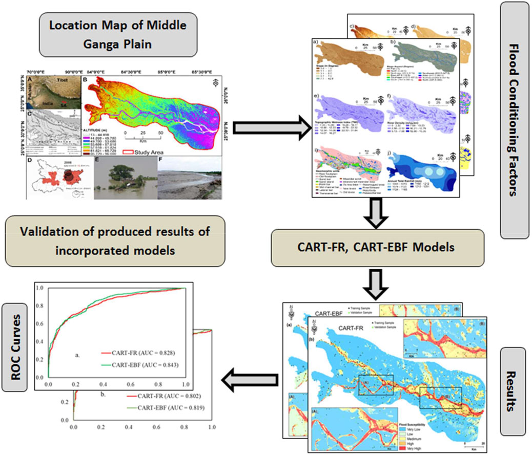
GRAPHICAL ABSTRACT
The recent developments in remote sensing satellite technologies and sensors (Toth and Jóźków, 2016; Zhang X. et al., 2019; Han et al., 2019; Weiss et al., 2020; Yang et al., 2021), rise in number of available platforms for the satellite data access (Boerner, 2007; Rizzato et al., 2020), and improvements in other low altitude geospatial technologies like lightweight unmanned aerial vehicles (UAVs) (Rizzato et al., 2020) have aided to ease the monitoring and analysis of natural hazards and disasters (Gillespie et al., 2007) at various spatial and temporal scales. Since monitoring floods in urban settings is difficult due to narrow open space among the concrete jungles, use of UAVs immensely helps to monitor and quantify the flooded and flood-induced damages (Yalcin, 2018). Challenges, advantages, and disadvantages of using UAVs for such purposes in urban settings are discussed in detailed fashion in the literature (Feng et al., 2015). Freely available remote sensing products such as optical, radar, and hyperspectral datasets are more popular in studies quantifying different aspects of natural hazards (Lin and Yan, 2016; Yao et al., 2019). These remote sensing datasets are used to monitoring of current flood events (Ban et al., 2017) and to compute different set of variables that are entered as input in flood prediction models (Arora et al., 2021a).
In recent years, modeling development has attracted the attention of many researchers in various scientific disciplines (Cheng and Han, 2016; He et al., 2018; Chen et al., 2021). Multi-criteria decision-making (MCDM) (Opricovic and Tzeng, 2004; Abdullahi et al., 2015; De Brito and Evers, 2016; Turskis et al., 2019) and artificial intelligence (Suman et al., 2016; Guikema, 2020; Sun et al., 2020; Tan et al., 2021) models are very popular among researchers. There are a wide variety of flood inundation prediction models, e.g., statistical models including bivariate and multivariate (Tehrany et al., 2014), machine learning models, multi-criteria decision-making (MCDM) (Nachappa et al., 2020), and an ensemble of two or more models (Arabameri et al., 2020c). Guerriero et al. (2018) have discussed a more exhaustive discussion of existing methods on the flood inundation models prediction with their pros and cons. Also, new models are being devised and tested regularly (Razavi Termeh et al., 2018). However, different flood susceptibility models perform with different levels of accuracy and sensitivity (Bui et al., 2018) giving rise to inconsistency in model performances in different environmental settings. Currently, there appears to be a challenging task to find a model with a high level of predictability in diverse topographic and climatic settings. This task requires rigorous testing of various flood susceptibility prediction index (FSPI) models in different topoclimatic settings like low-relief floodplain environment with humid subtropical monsoon climate (Hong et al., 2018b) and mountainous high-relief rugged terrain with the semiarid climatic regime (Ahmadlou et al., 2018).
As pointed out in the previous paragraph, different types of susceptibility models accrue differences in accuracy and sensitivity in a similar or same topoclimatic setting. Furthermore, new models are constantly being developed and tested to achieve a better level of accuracy and sensitivity and to overcome disadvantages arising out of different factors discussed by researchers (Reichenbach et al., 2018). Additionally, the need to develop new models and test the previously developed ones in different settings is clearly visible in the hazard modeling community in the present decade (Panahi et al., 2021). To further this current practice among the hazard modeling community, we, in this study, present two new ensemble models and test their performance for a typical topoclimatic setting. We test the performance of one recently developed novel-advanced ensemble model viz. CART-FR and one new ensemble model (CART-EBF) developed for the first time by us to predict flood occurrences and delineate flood susceptibility zones in a region of the Middle Ganga Plain environment. We apply 12 widely used flood predictors namely geomorphology, altitude, slope, aspect, plan curvature, topographic wetness index (TWI), drainage density, distance to the river, distance from the road, soil type, annual rainfall, and landuse/landcover (LULC). This study also attempts to assess the contribution significance and efficiency of different flood predictors by using information gain (IG) method, through analysis of weightage rankings assigned by various ensemble models. This flood predictor ranking may assist flood hazard managers during the policy formulation and mitigation measures implementation.
2 Materials and Methods
2.1 Study Area
The part of the Middle Ganga Plain (MGP) investigated for flood susceptibility prediction, covering an area of ∼10,138.5 km2, in this study is located in between the Upper and the Lower Ganga Plains (Figure 1). It lies between latitude 25°14′48.00″N–26°14′24.60″N and longitude 83°51′46.19″E–85°45′3.25″E. About 55.4% of the GRB (Singh et al., 2007) is covered with a thick layer of alluvium brought and deposited by a dense network of streams. There are a number of tectonic structures, both in the deep basement and at the surface which produce surface geomorphic markers revealing continuous active tectonic activity in MGP (Singh, 1996). The Ganga plain is also undergoing subsidence as a result of tectonics as well as excess groundwater depletion (Sahu et al., 2010). The study area is drained by several tributaries including Gomti River, Ghaghara River, Gandaki river, and Kosi river (these tributaries join the Ganga from the left bank); and Yamuna River, Son River, and Punpun river (these join the right bank of the Ganga). This densely populated area has been on the constant radar of national disaster management agencies for very long.
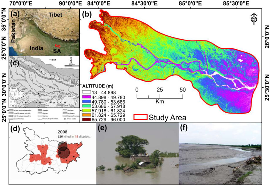
FIGURE 1. Location of the study area. (A): Location of the studied area marked on the map of India. It also shows Tibet and Pakistan in the northeastern and northwestern sides respectively. (B): Elevation of the study area classified using Natural Break (NB) method with input from SRTM 30m digital elevation model. (C): broad beological profile of the study area and its surroundings. This section also shows major drainages of the Ganga River Basin of which our study area is a part. (D) Loss of lives due to 2008 Bihar floods in 15 districts is shown here. (E,F) are photographs of the flood situation in the study area. (E,F): field photographs captured in the study area caused by 2008-Bihar flood.
GRB experiences a humid subtropical climate featuring four seasons—the winter season (January–March), summers (April–May), monsoon (June–September), and post-monsoon (OctoberDecember) (Dimri, 2019). According to the Indian Meteorological Department (IMD), the average annual mean, maximum, and minimum temperature experienced in GRB in 35 years (1969–2004) are 24.82°C, 31.22°C, and 18.44°C, respectively.
The MGP records average annual rainfall on the order of 100–120 cm, three-quarters of which is downpoured within 4 months long monsoon season (Trivedi et al., 2019). The influence of western disturbances (WDs) on Indian monsoonal rainfall is well-documented in the form of sporadic rains and hailstorms during the southward migration of intertropical convergence in winter months (Dimri and Chevuturi, 2016). The seasonal variability in the Ganga River discharge has led hydrologists to term river discharge of Indian River Network systems associated with monsoon systems such as monsoonal discharge, post-monsoonal discharge, summer or winter monsoon discharge (Gupta, 1984). The monsoon season river discharge in the Ganga River increases by 50–100 times due to heavy rainfall downpour.
2.2 Data and Methodology
Data preparation is the first step in scientific works (Feng et al., 2020). Table 1 provides the datasets used for preparing the flood predictors derived from Shuttle Radar Topography Mission (SRTM) digital elevation model (DEM) (30 m resolution), and other data sources, and flood inventory computed from Landsat-5 thematic mapper (TM) satellite imagery. The flood occurrence susceptibility modeling flow diagram shown in Figure 2 suggests that this research work has been accomplished in the follwing six steps: 1) obtain least cloudy Landsat 5 TM images of the study area from National Aeronautical Space Agency’s (NASA’s) earth explorer portal (https://earthexplorer.usgs.gov/) and generate the flood polygon for the “2008 Bihar Flood” event using normalized difference water index (NDWI) thresholding. The input datasets used in this study have been discussed in detail in Section 2 and its subsections in the study by Arora et al. (2021b), 2) create the flood inventory and the flood predictors, 3) generate flood and non-flood points for model training and validation, 4) test the conditioning factors of flood and non-flood points for multicollinearity, and also, apply the feature selection methods on all the flood predictors for a proper understanding of the suitability and contribution potential of all the factors involved. Here, we have applied information gain, 5) calculate the weightage of all the flood predictors using bivariate frequency ratio and evidential belief function models; also, devise the ensemble models with MLP, and CART machine learning models; and 6) perform model evaluations using various statistical parameters (discussed in the respective sections).

TABLE 1. Satellite and DEM data characteristic details used in the study.
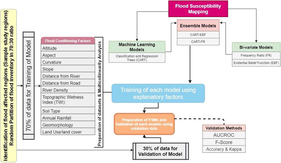
FIGURE 2. Flow diagram showing step-by-step methodology employed in this study.
2.2.1 Flood Inventorying
As suggested by Arora et al. (2021b), this step involves the computation of NDWI from the selected satellite scenes. The details of NDWI computation method, based on Gao (1996), are presented in Arora et al. (2021b). Flood pixels are separated from non-flooded pixels by applying a threshold ≥0.20 to the NDWI raster.
2.2.2 Flood Predictors
We have selected 12 flood predictors (Table 2) based on an extensive literature survey and our knowledge of the geomorphic, hydrologic, and climatic conditions of the study area. The slope angle is defined as the rate of change of elevation with Euclidean distance. Slope is one of the factors that determine and influence soil type, moisture content, and vegetation and, therefore, affects the surface runoff (Yang et al., 2020) and infiltration rates (Nassif and Wilson, 1975; Liu and Singh, 2004). Thus, the slope has both indirect and direct effects on flood inundation (Al-Rawas and Valeo, 2010). We computed the slope degree using ArcGIS 10.3 and DEM data and classified the slope range of 0–42.80° into five categories using the natural break method (Figure 3A).
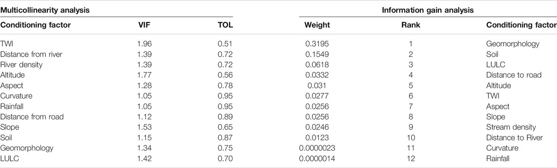
TABLE 2. Multicollinearity test results of all the conditioning factors; information gain (IG) attribute evaluation method for selection of flood conditioning factors using 300 flood and 300 non-flood points in Weka Software.
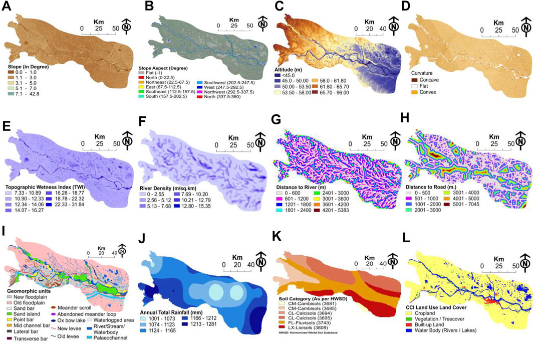
FIGURE 3. Flood conditioning factors used for modeling of flood susceptibility. From (A–L) the maps indicate Altitude, Slope; Aspect; TWI; River Density; Distance to Road; Annual Rainfall (mm); Soils; Curvature, Distance to River; LULC; and Geomorphology.
Slope direction is one of the variables that bear a relationship with the availability of soil moisture, geomorphic stability, exposure to radiation at the surface, wind (dry or wet), and rainfall intensity. Hence, it has an established relationship with flooding (Siahkamari et al., 2018). We used 3-D Analyst of SRTM DEM in ArcGIS 10.3 to calculate slope direction and categorized it into ten classes (Figure 3B).
Altitude affects the flood level in two ways: 1) elevation from the channel bed level decides how far from the rivers will inundation occur and 2) height from sea level controls atmospheric phenomena and hence type and magnitude of precipitation. In this study, SRTM v.4 30 m digital elevation model (DEM) derived low altitude range (13–96 m) surface of the area is classified into seven categories using the natural break method (Figure 3C).
Plan curvature or planform curvature is the directionality parallel to the maximum slope and decides the flow direction (Kimerling et al., 2016). We have used SRTM DEM to compute and reclassify three categories of planform curvature namely negative, zero, and positive indicating concave, flat, and convex surfaces, respectively (Figure 3D).
TWI is a quantitative measure indicating topographic control on hydrological processes. It is computed using the formula:
River density also known as drainage density (
Euclidean distance from the river channel is an important factor determining the extent of the inundated area by a flood (Khosravi et al., 2018). The areas far away from the river channel in a watershed are less probable to flooding than the ones nearer to the channel. Relationship of flood susceptibility to the distance to the river channel is subjective as the relationship varies from place to place depending on various factors (Choubin et al., 2019). We calculated the Euclidean distance to river channels in the Spatial Analyst Toolbox of the ArcGIS 10.3 and later interpolated and reclassified it into 10 categories to produce the map of “distance to the river” (Figure 3G).
Distance from the road is one of the important independent variables used in flood susceptibility modeling. The road networks in modern-day urban agglomerations increase impervious surfaces which contribute to changing the surface hydrological properties. Road network data used in this study have been obtained from Open Street Map Portal which is a collaborative mapping project (CMP). The data quality and its usability are described in Fan et al. (2014). After producing the map using interpolation, the data have been reclassified into seven categories (Figure 3H).
Geomorphology is closely connected to flood susceptibility (Mokarram and Sathyamoorthy, 2016). Floods sculpture landforms by the processes of erosion and deposition. Sometimes, extreme flood events destroy the landforms formed by different geomorphic agents. Thus, the interrelationship between floods and landforms of different scales (spatial and temporal) is established since the dawn of geomorphology as a discipline. In this study, geomorphological units were extracted from Google Earth Pro© through onscreen digitization method at 1:500/1,000 scale. Seventeen microscale geomorphic units have been identified through the classification of the study area (Figure 3I). Fine-scale geomorphology being another proxy that connotes the effects of active tectonic activities and seismological perturbances in the surface has also been taken as one of the exploratory variables of flood susceptibility, but it has previously been ignored in flood susceptibility modeling community. Some of the geomorphic markers mapped in this area which represent effects of active tectonic activity include 1) asymmetrical meander belts (Leeder and Alexander, 1987), 2) abrupt scarp faces, 3) highly sinuous mountain fronts (Taloor et al., 2019), 4) unpaired terraces (Joshi et al., 2016), 5) unilateral migration (Latrubesse, 2015), 6) shifted fan lobes and terraces (Jolley et al., 1990), etc.
Climate change affects hydrological processes (Tian et al., 2020; He, 2021). Rainfall variations have an impact on flash flooding (Mahtab et al., 2018). Prolonged rainfall events or a set of short-interval events of different intensities and magnitudes often prompt floods. In this study, we have used the global CFSR annual rainfall dataset to extract rainfall conditions in the study area (Trivedi et al., 2019). The dataset is provided on a 1000 m spatial resolution which has been resampled to 30 m resolution data by using the nearest neighbor (NN) method (Figure 3J). The data range of 1,001–1,081 mm is reclassified into six classes using the natural break method.
Different characteristics of soil affect various hydrologic properties of the surface (Zhang et al., 2019b). Soil types with high permeability and high infiltration ratio show less susceptibility to flooding and vice versa (Krogh and Greve, 2006; FAO and ISRIC, 2012). Soil map produced by FAO and ITPS (2015) used in this study is resampled at 30 m resolution and classified into six categories (Figure 3K).
LULC can alter and control factors such as moisture retention capacity of the surface, infiltration rate, surface runoff, heat albedo and hence bears a well-known relationship with flood possibility in an area. For example, if an area has been converted to built-up land from forested land, the probability of flooding increases owing to the increased imperviousness caused by altered surface cover type (Rogger et al., 2017). The LULC data produced by climate change initiative (CCI) program of the European Space Agency (ESA) have been used in this study. The subset of LULC data obtained from ESA archived 300 m spatial resolution, annual worldwide dataset generated for the period 1992–2015 (Li et al., 2018), has been reprocessed using nearest neighbor resampling procedure at 30 m resolution (Figure 3L). The manual provided by the agency gives a full description of the dataset which readers can access to gain better knowledge (ESA, 2017).
2.2.3 Multicollinearity Assessment Through the Variance Inflation and Tolerance Analysis
Multicollinearity analysis (Alin, 2010) (also known as collinearity) is the foremost important step in the regression analyses. The concept of multicollinearity refers to the property of predictor variables not showing dependency on one another which Dormann et al. (2013) phrase as “non-independence of the predictor variables.” The noncollinear relationship among flood predictors (or independent variables/predictor variables) is warranted to get unbiased model results. Collinearity among the predictor variables is determined through “variance of inflation (VIF)” and “tolerance (TOL)” for a case
where
2.2.4 Feature Selection Method for Flood Predictors
For determination of the significance of controlling factors and ranking flood predictors as per their contribution in the prediction of flood phenomena, the information gain (IG) method (Section 2.2.4.1) was applied using the Weka software v3.9.4, developed by the University of Waikato, Hamilton, New Zealand.
2.2.4.1 Information Gain
IG is one of the most widely used methods of feature selection in various machine learning (ML) applications including landslide modeling (Đurić et al., 2019) and flood modeling (Costache and Tien Bui, 2019). This method is found to be one of the fastest and simplest methods used for ranking the features (Hall and Holmes, 2003).
The concept of entropy is one of the main tenets of the “information theory” and serves as the basis of IG:
where
This equation assumes that
The decision of flood predictor selection using the IG based on entropy values of variables computed from D training dataset comprising n number of flood predictors can be expressed as follows (Chapi et al., 2017):
3 Models Employed for Flood Susceptibility Prediction Index Mapping
For the present work, two base bivariate statistical models, viz. FR and EBF, have been used to compute weightage for each of the twelve flood predictors. Subsequently, those flood predictors’ weight values have been used to train the ensemble advanced ML models namely CART, FR, and EBF models. In the subsequent subsections, the brief functionality of each of the individual models is described, and later, how the two bivariate model-based weights are used for ensembling the other three machine learning models is presented.
3.1 Models Applied for Data Preparation
3.1.1 Evidential Belief Function
This algorithm is based on Dempster-Shafer’s theory of evidence (Dempster, 1967; Smith and Shafer, 1976). Four important functions form the EBF: 1) belief function (Bel), 2) plausibility function (PLs), 3) disbelief function (Dis), 4) uncertainty function (Unc).
where
The above equation yields the Bel (belief function) calculated with the help of the following equation (Park, 2011):
where
The disbelief function (Dis) can be derived as:
And the following equations are used to compute uncertainty (Unc) and plausibility (PLs):
3.1.2 Frequency Ratio
Frequency ratio is a frequently used bivariate statistical model. It represents the probability of event occurrence; in our case, the event is the flood pixel (Arabameri et al., 2019b).
The frequency ratio (FR) computation uses the following mathematical expression:
where
3.1.3 Classification and Regression Tree
CART is a powerful data mining machine learning nonparametric algorithm proposed by Breiman et al. (1984). As the name suggests, it can perform both the classification and regression of number, binary, and categorical type of variables (Haughton and Oulabi, 1993). After performing the classification of variables in either number, binary, or categorical format, the average response values are computed using the mathematical expression:
where k = index of the target classes;
The resulting outcome of the CART model comes in a very complex form of a decision tree which needs pruning to extract only relevant and most important info out of it.
3.2 Ensemble Models Applied for Flood Susceptibility Prediction Index Computation
Due to the limitations of stand-alone models (Hapuarachchi and Wang, 2008; Hapuarachchi et al., 2011) and the advantages of ensemble models (Fernández et al., 2018; Zounemat-Kermani et al., 2020), in recent years, the use of ensemble models has expanded among researchers (Fernández et al., 2018; Zounemat-Kermani et al., 2020; Costache et al., 2021). Two ensemble models are used to derive the Flood Susceptibility Prediction Index and corresponding zonation maps. These ensembles are generated through the combination of CART and bivariate statistics models—FR and EBF. The factor class/category coefficients derived with the help of FR and EBF models are used as input in the CART.
3.3 Database Establishment
For the present research work, a database consisting of 12 flood predictors for a total number of 300 flood points was prepared using ArcGIS. Since the flood-prone area identification was performed following a binary classification of pixels, it was necessary to create another data sample, having the same number of points (300), consisting of non-flood locations (Ali et al., 2020). To ensure the objectivity of the results, the non-flood locations were randomly distributed across the entire study area.
3.4 Feature Selection With IG
The involvement of multiple predictors to estimate the susceptibility to a specific natural hazard can lead to issues related to the prediction (Costache, 2019). To overcome this shortcoming and to eliminate the noisy data from the workflow, the predictive ability of the 12 flood predictors was tested using information gain (IG). To determine the flood predictors’ significance, all the three models were applied using Weka 3.9 software.
3.5 EBF and FR Coefficient Normalization
EBF and FR coefficients were used to code the predictor class/category. These two types of coefficients were calculated using the procedure described in Sections 3.1.2, 3.1.3. Furthermore, to bring the EBF and FR values to the same range of values, the normalization procedure was applied using Equation 23 proposed by Costache et al. (2020):
where
3.6 Preparation of the Training and Validating Datasets
After obtaining the normalized EBF- and FR-derived weightage database, we need to set up the training and validation samples using this newly generated dataset. Previous studies (Arabameri et al., 2019a; Bui et al., 2019a) suggest that the training sample is established to represent 70% of the total dataset, while the other 30% is apportioned for validating the dataset. Thus, we used 210 flood and 210 non-flood pixels as the training dataset, while 90 flood and 90 non-flood locations were used in the validation process. The Subset Features tool from ArcGIS was used to randomly split the dataset.
3.7 Setting the Configuration for Hybrid Ensemble Models
3.7.1 CART-EBF and CART-FR Ensembles
The two CART-based ensembles were trained with the help of Salford Predictive Modeler v8.2 (Costache et al., 2020). The trial process was used to optimize the CART ensembles’ parameters (minimum cases of parent nodes and terminal nodes) whose values were established in accordance with the highest AUC. Finally, the weights of the flood predictors for CART-EBF and CART-FR ensembles were also determined.
3.8 Model Performance Evaluation and Comparison
Performance evaluation is the most important step in scientific works (Zhang et al., 2019a). Because no single or a set of universally valid model evaluation measurement matrices related guidelines could be found such as AUROC, TSS, RMSE (Zhou et al., 2018; Alam et al., 2020), and others, we have chosen two types of matrices to evaluate the performance of models used in this study: 1) threshold-independent and 2) threshold-dependent. Under the first category, area under the receiver operating characteristic (AUROC) curve has been used. In the case of the threshold-dependent performance evaluation matrix, we have used true skill statistics (TSS) and others (see Table 6). It should be noted that many of the threshold-dependent matrices (West et al., 2016) listed in Table 6 are derived from AUROC curve (the abbreviations used in this section are given in Table 6 and its appended note given just below the table).
The AUROC graph plot is a biaxial plot with “sensitivity” (y-axis parameter) versus “1-specificity” (x-axis parameter) (Jiménez-Valverde, 2012). The AUROC value ranges from 0.5 (inaccurate) to 1 (highly accurate).
The matrices plotted on the two axes of the ROC curve, sensitivity (also called true positive rate), and specificity (or true negative rate) are expressed in mathematical form as:
where
The specificity and sensitivity values using different cutoff thresholds for both models CART-EBF & CART-FR are provided in Table 4.
The threshold-dependent statistic metric used in this work, the “true skill statistics (TSS)” (Flueck, 1987), is one of the popularly used skill score measures for categorical datasets in forecast-related studies. This matrix’s discovery traces back to its first proposal by Peirce (1884) and is also widely called by the name “HanssenKuipers” discriminant (Wilks, 1995)/or Kuipers’ performance index/or the true skill statistic (Allouche et al., 2006). Cohen’s Kappa is dependent on the prevalence of sample points affecting the sensitivity and specificity of the model performance, and the TSS overcomes this disadvantage (Allouche et al., 2006). Besides, the accuracy, F-score, Cohen’s kappa (Cohen, 1960), Matthew’s correlation coefficient (MCC), TPR (sensitivity), TNR (specificity), FPR (fall out), informedness (bookmaker informedness; BMI), etc. (see Table 6 and the appended notes for details of the list of matrices and their expansions and calculation formulas) are also dependent on independent variables that control AUROC, such as TP, TN, FP, and FN have also been calculated for the performance evaluation of the models. All the performance evaluators (statistic matrices) listed in Table 6 are used for assessing different facets of model performances viz. accuracy, precision, robustness, sensitivity, consistency, the goodness of fit between observed and estimated values of natural phenomena, most of which are derived from the 2Χ2 contingency confusion matrix generated from binary classification scheme. There is a long list of classifier performance evaluation matrices. However, their suitability for a particular type of modeling exercise has not been put forward by the ML community yet (Seliya et al., 2009). Seliya et al. (2009) studied twenty-two of such evaluators with their meanings, what their higher or lower values imply as well as the relationship among them.
The Kappa statistic assesses the agreement between two distinguished sets of classification while catering to the randomness in the classification (Baattrup-Pedersen et al., 2012). The Kappa statistics can be calculated using the following equation:
where
The value of k-index varies between 0 and 1; the value moving towards 0 indicates less agreement, whereas those moving towards higher values, i.e., towards 1 indicate the model’s prediction accuracy heading towards or near to perfection. Cohen (1960) presented fivefold classification of k-index such that: K ≤ 0 (no agreement); 0.01–0.20 (slight agreement); 0.21–0.40 (fair agreement); 0.41–0.60 (moderate agreement); 0.61–0.80 (substantial agreement), and 0.81–1.00 near to perfect agreement.
We have also employed the seed cell area index (SCAI), and frequency ratio plots (FRP) for classification accuracy assessment of the models as the second round of validating the modeled classification results. The SCAI index computation takes into account the mathematical expression equating the ratio of each classified class and the susceptible seed cell percent values (Süzen and Doyuran, 2004):
where
4 Results
4.1 Selecting the Flood Predictors
We selected a list of flood predictors based on an extensive literature survey and familiarity with the topographic, hydrologic, climatic, and anthropic settings of the study area. Afterward, we selected the most significant and least redundant features or flood predictors by applying three statistical measures meant for checking multicollinearity, retrieving weights, and ranking of the variable features. We also analyzed interdependence among the flood predictors by applying the test of multicollinearity; furthermore, the application of IG (Figure 4) test methods has helped in ranking the flood predictors in order of their contribution to the flood occurrence probability.
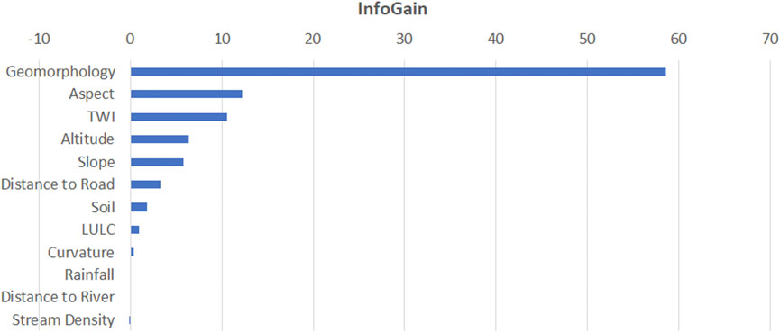
FIGURE 4. Importance of flood predictors derived through the use of IG arranged in order of their contribution to flood occurrence prediction.
4.1.1 Multicollinearity and IG Analyses of Feature Selection
Interdependency of flood predictors has been assessed by applying multicollinearity analysis. This analysis shows that all the flood predictors listed in Table 2 have variance inflation factor (VIF) and tolerance (TOL) > 10 and <0.1, respectively, which do not show sign of collinearity and hence can be included in the models applied for flood susceptibility zonation exercise.
The IG method applied to retrieve weightage and ranking shown in Figure 4 helps to assign rank to the flood predictors and is given in Table 2. The calculated IG ranks and weightages have ascertained the significance of the role of predictors in flood occurrence prediction. Geomorphology has been found to be the first ranker signifying its most important contribution in the flood susceptibility prediction process. IG method suggests that the first four most important flood predictors (descending order) are non-DEM-derived factors viz. geomorphology, soil, LULC, and “distance-to-road.” And the least significant predictors (increasing order of significance) are rainfall, curvature, “distance-to-river,” and stream density. As per IG, almost all the DEM-derived topography-related parameters, except curvature, are middle-level performants in their significance to flood contribution.
4.1.2 EBF and FR Coefficients
The FR and EBF model results for each class of every flood predictor have provided base weight values for training and validating data points for CART model ensembles. At first, we classified all the flood predictors’ values using the methods listed in Table 3. Subsequently, the EBF and FR weights corresponding to the original class values for each of the flood predictors at the subclass level were computed using methods discussed in Sections 4.1.1, 4.1.2, respectively. The elevation class ranges “0–45.0” and “65.8–96.0” show maximum (FR = 3.29; EBF = 0.39) and minimum (FR = 0.03; EBF = 0.01) weights for both FR and EBF, respectively. The slope aspect classes that provide maximum (FR = 1.54; EBF = 0.17) and minimum (FR = 0.68; EBF = 0.08) FR and EBF weights are flat (−10–00) and northwest (292.50–337.50). Out of the three curvature classes, class range assigned as flat gives the maximum FR (1.11) and EBF (0.37) weights whereas “convex” class renders the minimum weight for both FR (0.88) and EBF (0.30) models. The flood predictor “distance from river” class ranges which produced maximum (FR = 1.46; EBF = 0.40) and minimum (FR = 0; EBF = 0) weights by FR and EBF models are “0–600” and “3,601–4,200” as well as “4,201–5,383.” The FR and EBF models have assigned maximum (FR = 5.65; EBF = 0.33) and minimum (FR = 4.95; EBF = 0.29) weights to levee and waterlogged areas, two geomorphological classes, respectively. It can be noted that the maximum (FR = 3.30; EBF = 0.54) and minimum (FR = 0.18; EBF = 0.03) FR and EBF weight, respectively, have been assigned to “water” and “settlement” classes. The FR maximum and minimum weights for “rainfall” classes are 1.32 and 0.84, and as per EBF for the same “rainfall” classes, the value ranges from 0.24 to 0.15, respectively. As per FR and EBF, the maximum (2.62) and minimum (0.74) weights for river density have fallen in the same classes as 0.29 (max) and 0.08 (min), respectively. In the case of “distance to road” flood predictor classes “3,001–4,000” and “0–500,” maximum and minimum weights computed using FR are 2.02 (max) and 0.60 (min); and that by EBF are 0.25 (max) and 0.07 (min), respectively. The maximum (FR = 2.46; EBF = 0.34) and minimum (FR = 0.86; EBF = 0.12) FR and EBF weights delivered to account for the “slope angle” classes viz. “7.1–42.8” and “1.1–3.0” and “3.1–5.0”, respectively. Fifth soil class (FL-Fluvisol-3743) and third soil class (CL-Calcisol-3694) were recognized as maximum (1.78) and minimum (0.16), respectively, by FR; and that by EBF model, weightage values are 0.44 as maximum and 0.04 as a minimum. TWI class (22.33–31.84) has been the one with maximum weight value for both FR as well as EBF (FR = 4.41; EBF = 0.35); and the TWI class “7.33–10.89” is representative of minimum (FR = 0.80; EBF = 0.06) weight as per FR and EBF both. Classwise weights of each class of every flood predictor for FR and WBF are tabulated in Table 3.
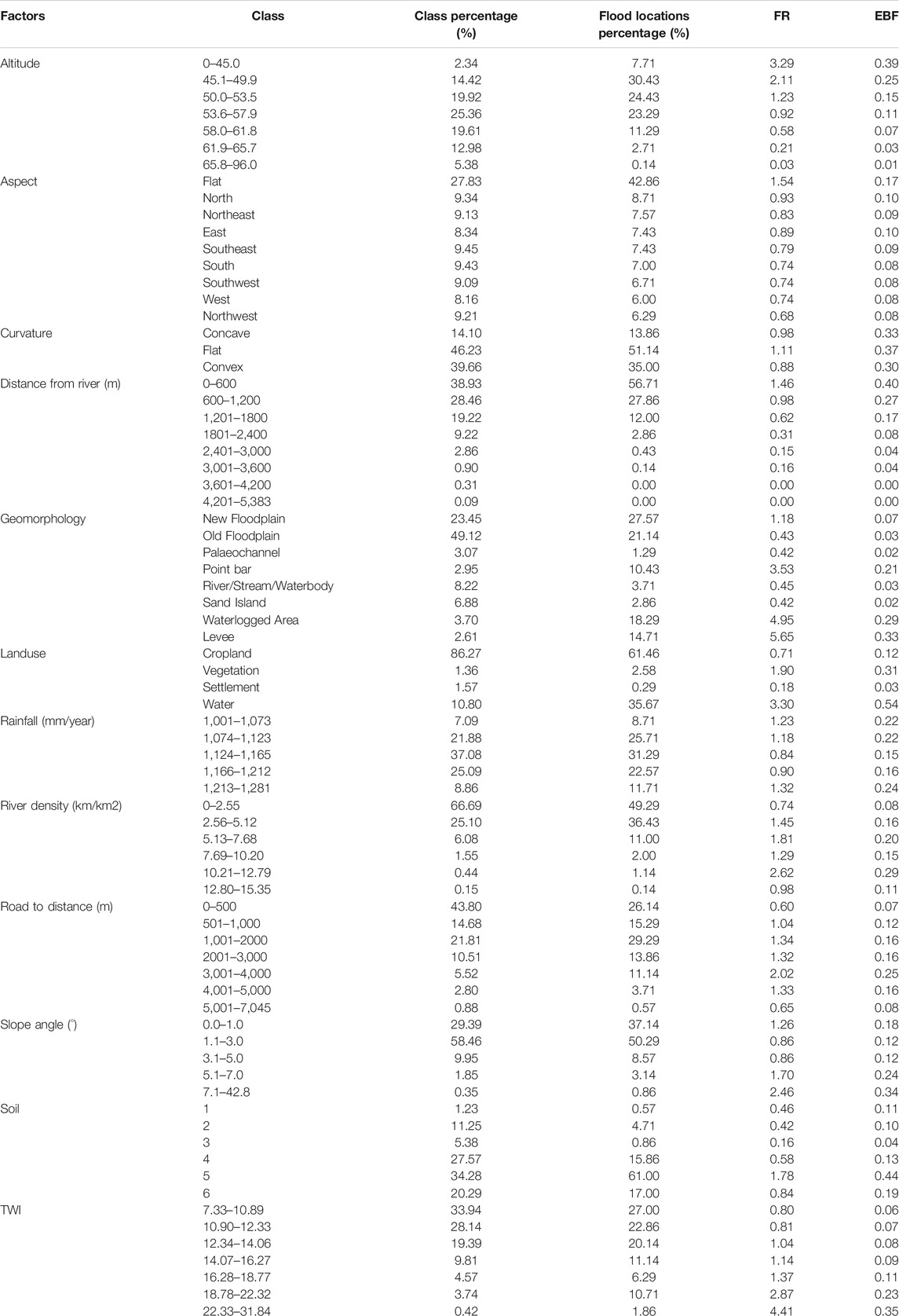
TABLE 3. FR and EBF values of factor class/categories (FR values taken from Arora et al., 2019b).
4.1.3 Flood Susceptibility Prediction Index Zonation Results
All the hybrid models were trained and validated using normalized flood predictor values for each class representing the controls of flood susceptibility in the MGP (see Section 3.6). After estimating the FR- and EBF-based flood predictor weights of the entire 600 flood and non-flood points, the trial-and-error method using backward and forward propagation was applied to obtain the CART ensemble weights for those points. Four categories of results were obtained by the use of EBF- and FR-based ensembles: 1) the ensembles have arranged the flood predictors in the sequence of their significance (ascending order of weight assigned to the flood predictors); 2) by using these weights for each subclass of every flood predictor, the flood susceptibility prediction index (FSPI) of the entire study area was obtained and classified into “very low,” “low,” “medium,” “high,” and “very high” flood susceptible zones using natural break (NB) method (Figures 5A,B); 3) corresponding to each class of FSPI, the entire study area was delineated into 5 zonation units (with the percentage of area appendages to each class) (the areal share of each FSPI zone using four different segmentation methods is presented in Figures 6A–C); and 4) the accuracy, sensitivity, precision, robustness, etc. of all the models indicating how well the models performed in this low-relief, subhumid monsoon-dominated topoclimatic setting have been computed. For both of the ensembles, these different levels of results are presented in the subsections below. Since the natural break (NB) method is most widely used and quantile (QNTL) accrued the highest areal percentage shares in the “high” and “very high” classes, FSPI % shares were separately computed for all the methods using these two methods and are presented in Figures 7A,B.
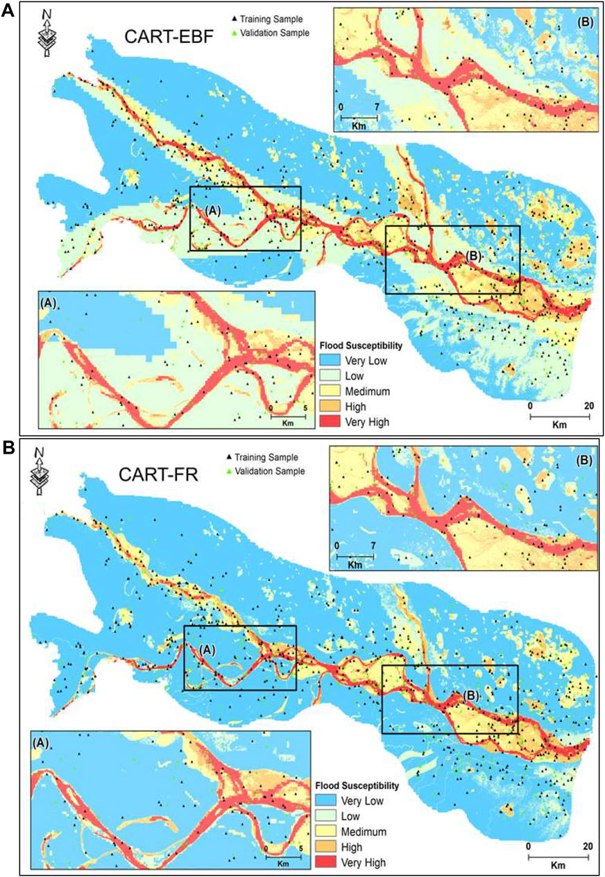
FIGURE 5. Flood susceptibility map using six ensemble models computed using methods discussed in Section 5.1; (A, B) show FSPI classified results according to CART-EBF and CART-FR results. Boxed areas A and B are zoomed windows in each of the model output maps to show detailed FSPI conditions nearby confluence zones.

FIGURE 6. FSPI histogram classification of both models’ outputs. In parts (A) and (B), Percentage share of areal coverage in “very low,” “low,” “medium,” “high,” and “very high” categories as classified by Natural Break (NB) and Quantile (QNTL) methods, respectively, is visualized, whereas, in part (C), areal coverage (%) by using four methods (EI-Equal Interval; GI-Geometric Interval; NB-Natural break; and QNTL-quantile) for only “high” and “very high” classes is demonstrated.
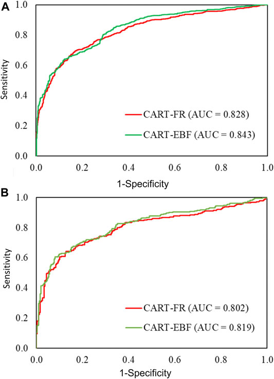
FIGURE 7. Area under receiver operating characteristics (AUROC) curve for the model was constructed in a single graph in order to compare the model’s performance. Validation of the models was performed using 30% of the randomly generated flood points specifically segregated from the points kept for the purpose of validation using AUROC statistical method. Panel (A) is computed using training dataset (represents model success rate) and Panel (B) with validation datasets (shows model prediction rate).
4.1.3.1 CART-EBF and CART-FR
Following the training procedure keeping in mind different cut-off thresholds corresponding to specificity and sensitivity values of both the models (Table 4), the minimum cases of parent nodes for the CART-EBF ensemble were established at 24, while the minimum cases of terminal nodes were kept equal to 10. Instead, in terms of the CART-FR model, the optimal minimum cases of parent nodes resulted to be 27, while the optimal minimum cases of terminal nodes were 12. Based on these details, the models, in the next step, have computed the weights for each of the flood predictors which are arrayed in Table 5. According to this Table 5, the CART-EBF and CART-FR have, computationally, annexed the “land use” (0.115) and the “geomorphology” (0.125) as highest weight scorers, respectively, followed by soil (0.114), geomorphology (0.111), altitude (0.073), TWI (0.021), aspect (0.020), river density (0.019), distance from river (0.015), road distance (0.015), rainfall (0.01), curvature (0.002), and slope angle (0.001) as per CART-EBF, and altitude (0.121), land use (0.054), soil (0.046), rainfall (0.039), distance from river (0.024), TWI (0.014), aspect (0.008), river density (0.007), curvature (0.005), road distance (0.004), and slope angle (0.002) according to CART-FR.
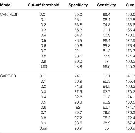
TABLE 4. Specificity and sensitivity values using different cut-off thresholds.
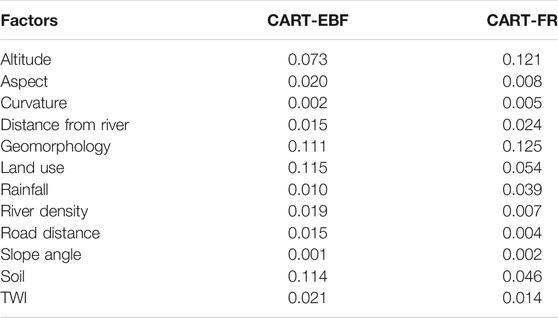
TABLE 5. Weights of conditioning factors within the applied models.
By applying these flood predictors’ weights, the FSPI values were computed in raster calculator embedded in Spatial Analyst of ArcMap version 10.3 and categorized into 5 classes for carrying out flood zonation using four classification methods QNTL, NB, GI, and EI. The highest percentage share of flood pixels in the “very high” class category has been noted by QNTL (19.43%), and the second, third, and fourth rankers stood out to be GI (9.94%), NB (8.14%), and EI (3.81%) for CART-EBF. And for CART-FR, the first rank has been registered by QNTL (19.64%), followed by the lower rank holders in descending order as GI (5.11%), NB (3.92%), and EI (0.89%) respectively.
4.2 Model Performance Validation Through AUROC and Other Statistical Measures
In Table 6, model performance evaluation statistic matrices belonging to two categories of evaluators viz. cutoff-dependent, cutoff-independent, most of which are derived from confusion matrix related parameters, such as TP, TN, FP, and FN, are presented. These are used to assess different aspects of model performances, such as model accuracy or efficiency, precision, robustness, randomness driven performance, etc. Rahmati et al. (2019) reviewed 21 threshold-dependent model performance evaluation indices to judge different aspects of the functioning of susceptibility models used in the field of natural hazard studies. We have used only 14 of those evaluators (given in Table 6) to refrain from making model evaluation sections of the paper lengthy. As suggested by Rahmati et al. (2019), the threshold-independent and threshold-dependent evaluators used in this work are discussed in the following Sections 4.2.1, 4.2.2, respectively.
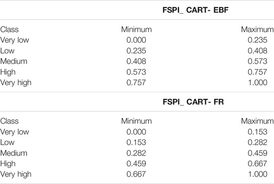
TABLE 6. Minimum and maximum FSPI values for all the flood susceptibility classes as per CART- EBF and CART-RF models.
4.2.1 Threshold-independent Matrices
Area under receiver operating characteristic (AUROC) curve, success rate curve (SRC: ROC computed using training dataset), and prediction rate curve (PRC: ROC computed using validation dataset) for all the modeled results are given in Figures 7A,B and Table 4. For the training dataset, CART-EBF (84.3%) has performed better than CART-FR (82.8%), whereas AUROC concept applied to the dataset used for validation of models results in a higher prediction rate for CART-EBF (81.9%) and slightly lower for CART-FR (80.2%).
4.2.2 Threshold-dependent Matrices
All 14 threshold-dependent evaluation matrices are presented in Table 4. The detailed definition, formulae, and their interpretation are given by Frattini et al. (2010) and Rahmati et al. (2019). In terms of the overall accuracy of ensembles (for both training and validation datasets), the CART-EBF (AccSR = 81.40%; AccPR=79.60%) outsmarts the CART-FR (AccSR = 75.9%; AccPR=74.0%). In this study, both ensembles have exhibited sensitivity (TPR: true positive rate or the ability of models to correctly predict positives or flood points) in the range of 78.5–82.4% for the training dataset and 76.0–80.9% for validation dataset. The models’ ability to correctly predict the negatives, i.e., non-flood points, is adjudged by the specificity or true negative rate (TNR) was found to be 0.738 for CART-FR for training dataset and for validation phases, and the TNR value is 0.723. The PPV (positive predictive value), also called as confidence or precision of predictive capacity of models, and its complementary metric FDR [false discovery rate, which deals with conceptualization of Type I error. See Frattini et al. (2010) for the definition of Type I and II errors] are used here to see how precisely the ensembles used here can predict flood pixels and non-flood pixels, respectively. The higher values of PPV and lower value of FDR are indicative of the high precision of prediction capability of ensembles. CART-FR with PPV: 0.714; FDR: 0.286 (for training data) and PPV: 0.783; FDR: 0.298 (for validation dataset) has been found to perform a little imprecisely than CART-EBF (Table 6). It should be noted that the lower the value of FNR, the better the model performance. Though accuracy and F1-score have been widely used to assess model performances, they sometimes lead to misleading implications. The F1-score does not take into account all the four primary matrices of the confusion matrix and that is where MCC (Mathew’s Correlation Coefficient) plays a decisive role as it overcomes this shortcoming by incorporating all the four matrices (Chicco and Jurman, 2020). A look at the F1-Score and MCC values of the ensembles in Table 6 reveals that when adjudged based on overall accuracy as well as F1 and MCC, the same sequence of performance levels emerges for both models. The k-index or kappa index, one of the most widely used statistic for model performance accuracy assessment, suffers from a lacuna involving its overdependence on prevalence or pervasiveness of samples (Allouche et al., 2006). Hence, to overcome this issue, an alternative measure, true skill statistic (TSS) has been computed and is presented in Table 6. According to k-index and TSS as well, when considered concomitantly, the CART-EBF model is the better accurately performing model during the training and validation phases than the CART-FR. Table 6 lists the “informedness” or “bookmaker informedness; BMI,” statistic referred to be the “only unbiased indicator” of model accuracy which helps with an informed selection of models.
4.2.3 SCAI- and FRP-Based Performance Evaluation
The second round of validation matrices, SCAI-, and FRP-based performance of both ensembles’ accuracy was performed to gain an extra level of confidence in model results. The computation of SCAI & FRP at the classwise level was performed as per methods discussed in Sections 3.8, 4.1.2, respectively. In this study, as visible in Figure 8B, CART-EBF (SCAI = 5.209 for “very low” class) performs more accurately than CART-FR (SCAI = 83.263 for “very low” class). The FRP-based performance in Figure 8A shows that the FR values of the lower class of both ensembles are lower, just opposite to the behavior of SCAI, and that of “high” and “very high” susceptibility classes are higher. This pattern of FPR classwise values conforms to the result implications provided by SCAI values; and that have presented a better confidence level about the models’ performance accuracy for both models.
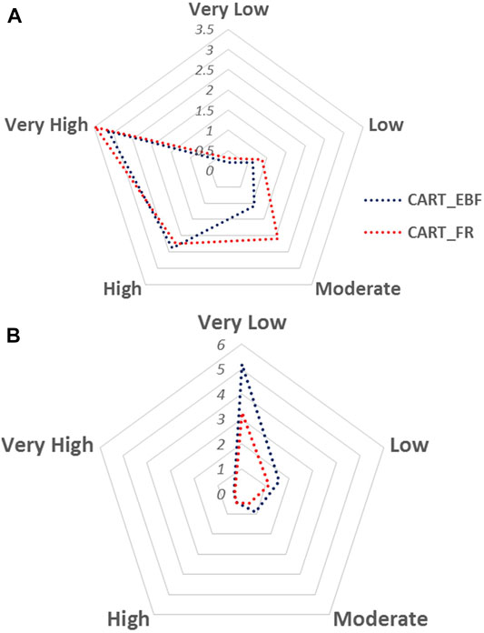
FIGURE 8. Ensemble model result validation using: (A) Frequency Ratio Plot (FRP); and (B) Seed Cell Area Index (SCAI) methods.
4.3 Flood Pixel Distribution Vis-à-Vis FSPI Classes
Figures 6A–C and Table 7 represent the final zonation of flood susceptible areas modeled by both the ensembles (classified using the natural break method). It shows areas highly susceptible (covering “high” and “very high” classes collectively) to flood menace and the safer zones. The FSPI values in the “high” and “very high” classes were used to compute the distribution of areas falling under these two classes (Figure 6). Since the QNTL has been found to delineate the highest percentage of areas under “very high” class, as discussed in Section 4.1.3, and in most of the published results, the final zonal classifications are performed by using NB, and the QNTL-based areal shares (in %) corresponding to the NB-based areal shares of “high” and “very high” classes are also shown and discussed here in this section using Figures 6A,B. The CART-EBF covers 27.24% areal coverage (as per NB classification method), whereas, as per the QNTL methods, CART-EBF encompasses 49.49% area under high and very high classes [see Table 7 (for FSPI) and Supplementary Table S1A for % areal coverage by each class]. The lower areal percentage coverage was produced by CART-FR (21.94% as per NB) and 29.49% as per QNTL.
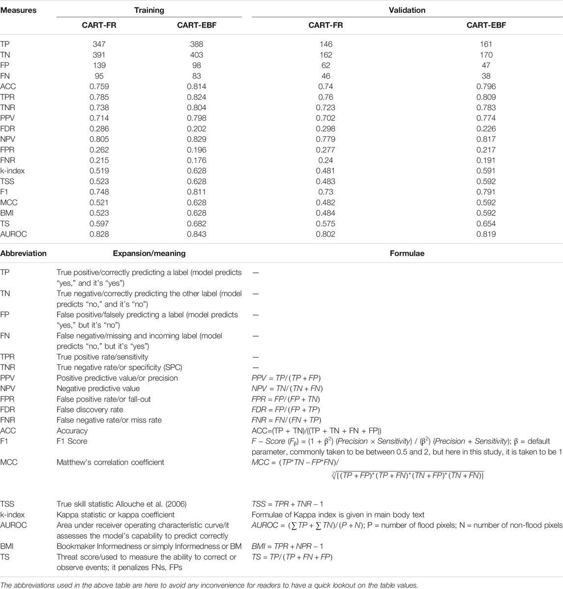
TABLE 7. Statistical metrices used for model performance evaluation (Note: All the abbreviations used in this table are expanded and defined below this table itself).
5 Discussion
5.1 Flood Predictor Significance
Predictor selection for the natural hazard susceptibility prediction aiming at determining the significance levels of contributing factors/control factors is done at three stages (Janizadeh et al., 2019). 1) First, multicollinearity analysis (VIF and TOL) is performed before training the models. This helps to root out all the interdependent control factors. 2) Then, orderly levels of contribution of control factors in computation of natural hazard susceptibility prediction indices (NHSPIs) are analyzed using the factor selection techniques such as IG, relief-F, RF. Control factors with weights higher than zero only are included in the model training and validation processes. 3) Finally, by application of all the models, weights are retrieved to all the conditioning factors. The second-stage results using IG were useful for winnowing out the flood predictors with zero weightage values to be included in the analysis even when their multicollinearity results of the first stage allowed them to be included for further step of the model training. The output from the third stage of the control factor is helpful at the policy formulation level in hazard management. The exact knowledge of the area-specific flood-predicting control factors will help hazard-related policy formulators to allocate funds that manage those respective flood predictors on a priority basis as compared to others. There are numerous techniques used for assessing the significance of contributing factors at aforesaid second and third stages. The type and number of conditioning factors (for floods) depend upon several variables including type topographic and climatic settings (Benson, 1963; Merz et al., 2014) as well as the type of flood, e.g., flash flood, precipitation-induced riverine flood, coastal storm flood, tsunami induced flooding (Pignatelli et al., 2009), or glacial lake outburst flood (GLOF) (Aggarwal et al., 2017)/landslide lake outburst flood (LLOF) (Srivastava et al., 2017). The quality of topographic data (Cook and Merwade, 2009) can also affect the predictor significance. High-resolution LiDAR-derived DEMs (Laks et al., 2017) and their derivatives behave differently than those which are derived using freely available DEMs, such as SRTM 30 m, ASTER 30 m, AW3D 30 m. For fluvial or riverine floods in mountainous areas, terrain parameters perform better when derived from ALOS World 3D 30 m (AW3D 30 m) (Boulton and Stokes, 2018), but the situation gets reversed for flat floodplain environmental setting like MGP (Tanaka et al., 2019). Since there is no specific guideline set for choosing the predictor significance assessment method and several previous studies use the medium resolution DEM dataset for deriving topography-based predictors (Santos et al., 2019), SRTM 30 m version 4 DEM-derived topographic variables were computed (see Section 2), and their significance was analyzed using IG. The results of this analysis show that detailed geomorphological mapping derived geomorphic units have played a very important role in flood susceptibility prediction using IG method. The second rank assigned to “distance to river” by this method appears to be true as the “2008 Bihar” flood, which is the source of flood inventory in this work, was a riverine flood due to overbank flooding caused by levee breach in the upstream Kosi megafan area leading to the sudden supply of water discharged for the lower reaches (UNDP Emergency Analyst, 2008). There was a time lag of around 10 days between the excessive rainfall in upper catchments, Kosi levee breach, and 2008 Bihar flooding (for which we have created our flood inventory), that’s why “rainfall” has scored least significance as a flood predictor. The reason for geomorphology bearing the first place on the significance score scale is that in the fluvial environments, most of the geomorphic forms evolve through processes governed by rivers’ hydrological, hydraulic, erosive, depositional, etc., characteristics. In a study conducted in the mountainous catchment of the northeast region, Lao Cai, of Vietnam, the DEM-derived predictor “slope angle” has received the highest predictive value whereas another DEM-derived parameter “curvature” was reported to be the least predictive factor (Bui et al., 2019a). The same study highlights that four other predictors, out of 12 used in that study, which have scored high significance scores, were DEM-derived parameters. In this study, four DEM-derived parameters: aspect, TWI, altitude, and slope have scored significant weights as per IG, equivalent to second, third, fourth, and fifth ranks, respectively. Irrespective of their apparent image of being dominant control factors of floods, rainfall could not stand among first five contributing factors in this study which conforms to the findings by other studies conducted in different parts of the globe (Tien Bui et al., 2020). Khosravi et al. (2019) conducted a study in a hilly moderate relief topographic setting (altitude range: 29–1,410 m) located in China and found that rainfall doesn’t have significant predictive significance. In their study, altitude scored the highest predictive significance followed by distance from river, NDVI, soil, slope, lithology, LULC, STI, rainfall, SPI, and curvature. There are variations in the significance scores of DEM-derived contributing factors such as slope, aspect, curvature, stream power index (SPI), terrain surface texture (TST), topographic position index (TPI), etc. and that may be because of a number of factors related to DEM resolution, algorithms used (IG, relief-F, RF, SWARA, etc.), type of topographic setting (plain or mountainous), number of factors used in the modeling exercise, etc. We could not find a study that has sorted out this issue of variability in the significance scores of conditioning factors due to the variability in data quality, use of different techniques/algorithms, number of conditioning factors, to name a few among others. Hence, there is a need for future research on this theme.
5.2 Nature of Flood, Predictor Selection, Topoclimatic Setting
The literature is replete with studies conducted with the aims of applying a new model for susceptibility prediction of different types of natural phenomena like floods (Ngo et al., 2018). Looking at the number and type of conditioning factors used by these studies, it appears that there is no clear guideline as to how many conditioning factors and which conditioning factors should be applied for, say, floods susceptibility, or landslide susceptibility, or ground subsistence susceptibility, or groundwater potential mapping exercises that can accrue to most optimal model performance. One common practice seen in the flood susceptibility modeling studies is that most of the researchers use “geology” or lithology as one of the control factors for flash floods, riverine floods, and storm surge related floods irrespective of whether they occur in mountainous regions, floodplain zones of low-relief settings, high mountain plateau provinces (Ngo et al., 2018), or coastal zones (Dodangeh et al., 2020), and in all these studies, the significance level of “lithology” stood out to (Di et al., 2019) be at sixth or later ranks. But there has been no study which employed detailed microlevel “geomorphology” as a control factor in low-relief topographic zone’s riverine flooding events. Selection of geomorphology as a proxy for flood susceptibility has been essentially chosen here because the area is affected by active tectonic perturbances, and continuous and fast groundwater depletion is causing ground subsidence. And geomorphology directly reveals those effects. Vegetation in different types of topographic and climatic settings shows the variance in their type (Kumar, 2016), and hence, vegetation diversity in different terrain types will alter the characteristics of NDVI and its threshold (Davenport and Nicholson, 1993). Keeping these associations between vegetation diversity changes and topoclimatic environmental variability, application of NDVI threshold may change its significance score, and hence, model performance too can follow suit.
5.3 Comparative Assessment of Ensemble Models’ Performance Vis-à-Vis Topoclimatic Setting
The EBF- and FR-based two ensembles with CART used in this work have yielded accuracy levels, as adjudged in terms of the threshold-independent statistics like AUROC, in the range of widely acceptable limits as per the classification scheme of AUROC values followed by Fressard et al. (2014). Both the ensemble models’ AUROC has been found to be within the range of 0.828–0.8432 (for training dataset) and 0.802–0.819 (for validation dataset). The higher AUROC, for both the training and validation datasets (also known as success rate or SR and prediction rate or PR of the model), has been scored by CART-EBF (SR = 0.843; PR = 0.819) and slightly lower by CART-FR (SR = 0.828; PR = 0.802) (Figures 7A,B). It is worth noting that this study has been performed in a low altitude (altitude range: <45.0–96.0 m AMSL) humid monsoonal climatic region undergoing constant active tectonic perturbances (Valdiya, 1976; Brown and Nicholls, 2015) and hence frequent and more severe flooding in the low-lying subsiding areas. In such a topographic environment, the use of moderate spatial resolution digital elevation data lends more levels of uncertainty errors which further propagate in other derivatives computed using this data (Oksanen and Sarjakoski, 2005). In such topographic settings, augmentation of topographic data quality has the potential to enhance the accuracy of DEM-derived input parameters (Sanders, 2007) and hence the models’ performances (van Westen et al., 2008). By applying the LR-, MLP-, and CART-based ensemble with a different bivariate model viz. statistical index (SI) for an area located in the mountainous and hilly part of Romania (altitudinal range: 242–1,463 m AMSL, characterized by temperate continental climate), Costache et al. (2020) have achieved both success rate and prediction rate accuracies of 0.94 (MLP-SI), 0.939 (CART-SI), 0.925 (LR-SI) and 0.927 (MLP-SI), 0.922 (CART-SI), 0.901 (LR-SI), respectively. There are 10 flood control factors selected by Costache et al. (2020), for flash flood occurrence prediction in his study area, and four out of them viz. L-S factor, hydrological soil group (HSG), stream power index (SPI), and topographic position index (TPI) are different from our study. In another study, Costache and Tien Bui (2019) investigated flash flood susceptibility prediction in different parts of Romania in similar topoclimatic setting for flash flood susceptibility prediction but with 14 flood predictors, five of which are different from ours, and achieved almost same levels of accuracy of success and prediction rates, as their previous study discussed just above in this section, but better than ours, ranging from MLP-FR (0.94), CART-FR (0.937) and MLP-FR (0.981), CART-FR (0.929), respectively. MLP-EBF trained and validated with 10 flash flood conditioning factors in hilly and mountainous catchment dominated by temperate climate has accrued 0.912 AUROC success rate accuracy and 0.806 prediction rate accuracy in identifying torrential valleys vulnerable to flash floods (Costache et al., 2019). In almost similar (similar to ours) flat terrain setting and climate, Hong et al. (2018a) have conducted a study wherein the altitude range was between <40–720 m AMSL in the southeastern part of China to investigate the fuzzy weight of evidence (fuzzy-WofE)-based ensembles with logistic regression (LR), random forest (RF), and support vector machine (SVM) using 11 conditioning factors, three of which differed from ours, but their reported success rate accuracy and prediction rate accuracy levels were in the range of 0.9519 (fWofE-LR)–0.9882 (fWofE-SVM) and 0.9652 (fWofE-LR)–0.9865 (fWofE-SVM), respectively. This study reveals that SVM- and fuzzy-WofE-based ensemble has the capability to perform much better, accuracy-wise, in like MGP topoclimatic setting, with freely available moderate quality DEM-like ASTER 30 m.
Other reasons that affect model performance levels include quality of flood inventory generated using different methodologies, like some use NDWI (Jain et al., 2005), mNDWI (Mohammadi et al., 2017) with different threshold values, or some other methods using various sensors of satellite datasets such as optical Landsat 7 ETM+ and Landsat 8 OLI imageries (Kumar, 2016), or radar data (Ward et al., 2014), and water surface DEM and bare-earth LiDAR DEM differencing (Guerriero et al., 2018). Variations in the number of flood and non-flood points meant for training and validation of models, resolution of DEM to derive topography-based flood predictors, and other related parameters also affect the flood inventory accuracy and hence alter the model performance. Regarding DEM data quality, Podhorányi et al. (2013) who have used LiDAR derived DEM data, have asserted that the DEM data quality has an inverse relationship with the level of uncertainties involved, i.e. better the data quality, lesser is the level of uncertainty in DEM derived parameters. And hence, for better performance of susceptibility models, higher quality DEM is warranted. On the other hand, Chen et al. (2020) have used freely available different DEMs in the spatial resolution range of 30–90 m (all derived by resampling of 30 m ASTER DEM), and they reported that DEM spatial resolution does not necessarily affect the susceptibility model results. It should be noted that the difference between Chen’s results and that of Podhorányi’s maybe because Chen has derived all the seven variants of DEMs from the same ASTER 30 m data whereas the latter created their DEM from point clouds collected using LiDAR which has proven excellent in several aspects over freely available moderate resolution DEMs (Goulden et al., 2014). Different statistic matrices presented here in this work indicate different aspects of model performances like how good the prediction accuracy is or how sensitive the model behaves and what is the overall performance of the individual ensembles or how badly the model fails to predict flood or non-flood pixels, and other such aspects.
6 Conclusion and Recommendations for Future Research
To achieve the goal of flood susceptible area zonation of MGP based on FSPI produced by applying different ensembles of models, this study is the next in the series of models’ testing after Arora et al. (2021b). This study, based on AUROC, has shown that the CART-based ensembles with bivariates EBF and FR perform reasonably well with both success and prediction. When it comes to utilizing moderate resolution-based conditioning factors, by using as less as 12 conditioning factors only, the decision of selecting ensembles for flood zonation mapping, which is an essential requirement for achieving sustainable development goals (SDGs) set by United Nations related to flooding, it is recommended that CART-EBF should be given priority over CART-FR. Different threshold-dependent statistic indices connote different aspects of model performances (detailed in references cited in Section 3.8), and based on user’s requirements, the researchers and agencies are recommended to make their choices. Another point that emerges out of the models’ output used herein is that both the models have their performance accuracies in the range of “good” as per the traditional AUROC classification scheme.
Detailed microscale geomorphic mapping is based on “geomorphology” as playing the best contributor in the susceptibility prediction mapping. The rank of geomorphology as number one in tectonically active areas and in fluvial floodplain areas affected by regular riverine flooding appears to be because this factor incorporates effects of active tectonic activity and ground subsidence related to excessive and fast groundwater depletion. Looking at its significance, it is advised that the government of concerned areas having similar topoclimatic setting first gets the areas geomorphologically mapped by using high-resolution satellite to be used as input in the flood susceptible zonation exercises. The research by Arora et al. (2021a) also vindicates this observation.
Some of the limitations faced in this work are: 1) instead of ground truth points collected using GPS in the field, we have used Google Earth Pro® for validation of non-flood points; 2) moderate resolution DEM used for computation of input flood predictions. Use of DEMs prepared using point cloud obtained with unmanned aerial vehicles (UAVs) or pulsed laser light-based LiDAR DEMs, or terrestrial laser scanning (TLS) device-based DEMs would have affected the model performance accuracy that affects the susceptibility zone percentage shares. The testing of all kinds of models, both standalone and ensembles, of all family of models, for instance, machine learning, statistical, multicriteria decision-making models highlighting their advantages and disadvantages as well as new model development is recommended to have a better understanding of optimality in the behavior of models. Since in the forthcoming future, the age is going to be of machines, space-based monitoring, and quantification of all natural and man-made phenomena with the best possible accuracy and precision will be the prime information that will be needed. In the coming future, the missions like surface water and oceans topography (SWOT) (Morrow et al., 2019) will be the need of the time to monitor all the phenomena including floods from space, and instantaneous susceptibility prediction zonation of areas will be instantly planned to be done in such missions at the control rooms of such missions. Model universalization by the selection of the best model through rigorous testing and validation of the available models of different genres performing with higher accuracy in a particular type of topoclimatic environmental setting will help guide such future missions.
Data Availability Statement
The original contributions presented in the study are included in the article/Supplementary Material, and further inquiries can be directed to the corresponding authors.
Author Contributions
AArora and MP: Conceptualization, database preparation, and model output presentation in map and graph chart form and manuscript writing; AA and RC: Modeling and analysis; NK, VNM, HN, JM, MAS, YR, SS, and UKS: Manuscript writing, enhancement, guidance during write up, and manuscript revision during first and second rounds of review.
Conflict of Interest
The authors declare that the research was conducted in the absence of any commercial or financial relationships that could be construed as a potential conflict of interest.
The reviewer NL declared a past co-authorship with the authors AA, AA, RC to the handling Editor.
Publisher’s Note
All claims expressed in this article are solely those of the authors and do not necessarily represent those of their affiliated organizations or those of the publisher, the editors, and the reviewers. Any product that may be evaluated in this article, or claim that may be made by its manufacturer, is not guaranteed or endorsed by the publisher.
Acknowledgments
The authors are grateful to the department of geography, JMI for allowing the GIS lab for carrying out the part of analyses. The lab facility at the Department of Civil Engineering, Chandigarh University, Punjab, is acknowledged for they have allowed some part of the work to be carried out therein. Any use of trade, firm, or product name is for descriptive purposes only and does not imply endorsement by the authors.
Supplementary Material
The Supplementary Material for this article can be found online at: https://www.frontiersin.org/articles/10.3389/feart.2021.659296/full#supplementary-material
References
Abdullahi, S., Pradhan, B., and Jebur, M. N. (2015). GIS-based Sustainable City Compactness Assessment Using Integration of MCDM, Bayes Theorem and RADAR Technology. Geocarto Int. 30, 365–387. doi:10.1080/10106049.2014.911967
Aggarwal, S., Rai, S. C., Thakur, P. K., and Emmer, A. (2017). Inventory and Recently Increasing GLOF Susceptibility of Glacial Lakes in Sikkim, Eastern Himalaya. Geomorphology 295, 39–54. doi:10.1016/j.geomorph.2017.06.014
Aghdam, I. N., Pradhan, B., and Panahi, M. (2017). Landslide Susceptibility Assessment Using a Novel Hybrid Model of Statistical Bivariate Methods (FR and WOE) and Adaptive Neuro-Fuzzy Inference System (ANFIS) at Southern Zagros Mountains in Iran. Environ. Earth Sci. 76, 237. doi:10.1007/s12665-017-6558-0
Ahmadlou, M., Karimi, M., Alizadeh, S., Shirzadi, A., Parvinnejhad, D., Shahabi, H., et al. (2018). Flood Susceptibility Assessment Using Integration of Adaptive Network-Based Fuzzy Inference System (ANFIS) and Biogeography-Based Optimization (BBO) and BAT Algorithms (BA). Geocarto Int. 34, 1252–1272. doi:10.1080/10106049.2018.1474276
Al-Rawas, G. A., and Valeo, C. (2010). Relationship between Wadi Drainage Characteristics and Peak-Flood Flows in Arid Northern Oman. Hydrological Sci. J. 55, 377–393. doi:10.1080/02626661003718318
Alam, M. M., Zhu, Z., Eren Tokgoz, B., Zhang, J., and Hwang, S. (2020). Automatic Assessment and Prediction of the Resilience of Utility Poles Using Unmanned Aerial Vehicles and Computer Vision Techniques. Int. J. Disaster Risk Sci. 11, 119–132. doi:10.1007/s13753-020-00254-1
Ali, S. A., Parvin, F., Pham, Q. B., Vojtek, M., Vojteková, J., Costache, R., et al. (2020). GIS-based Comparative Assessment of Flood Susceptibility Mapping Using Hybrid Multi-Criteria Decision-Making Approach, Naïve Bayes Tree, Bivariate Statistics and Logistic Regression: A Case of Topľa basin, Slovakia. Ecol. Indicators 117, 106620. doi:10.1016/j.ecolind.2020.106620
Allouche, O., Tsoar, A., and Kadmon, R. (2006). Assessing the Accuracy of Species Distribution Models: Prevalence, Kappa and the True Skill Statistic (TSS). J. Appl. Ecol. 43, 1223–1232. doi:10.1111/j.1365-2664.2006.01214.x
Arabameri, A., Rezaei, K., Cerdà, A., Conoscenti, C., and Kalantari, Z. (2019a). A Comparison of Statistical Methods and Multi-Criteria Decision Making to Map Flood hazard Susceptibility in Northern Iran. Sci. Total Environ. 660, 443–458. doi:10.1016/j.scitotenv.2019.01.021
Arabameri, A., Saha, S., Chen, W., Roy, J., Pradhan, B., and Bui, D. T. (2020b). Flash Flood Susceptibility Modelling Using Functional Tree and Hybrid Ensemble Techniques. J. Hydrol. 587, 125007. doi:10.1016/j.jhydrol.2020.125007
Arabameri, A., Saha, S., Roy, J., Tiefenbacher, J. P., Cerda, A., Biggs, T., et al. (2020c). A Novel Ensemble Computational Intelligence Approach for the Spatial Prediction of Land Subsidence Susceptibility. Sci. Total Environ. 726, 138595. doi:10.1016/j.scitotenv.2020.138595
Arabameri, A., Yamani, M., Pradhan, B., Melesse, A., Shirani, K., and Tien Bui, D. (2019b). Novel Ensembles of COPRAS Multi-Criteria Decision-Making with Logistic Regression, Boosted Regression Tree, and Random forest for Spatial Prediction of Gully Erosion Susceptibility. Sci. Total Environ. 688, 903–916. doi:10.1016/j.scitotenv.2019.06.205
Arora, A., Arabameri, A., Pandey, M., Siddiqui, M. A., Shukla, U. K., Bui, D. T., et al. (2021a). Optimization of State-Of-The-Art Fuzzy-Metaheuristic ANFIS-Based Machine Learning Models for Flood Susceptibility Prediction Mapping in the Middle Ganga Plain, India. Sci. Total Environ. 750, 141565. doi:10.1016/j.scitotenv.2020.141565
Arora, A., Pandey, M., Siddiqui, M. A., Hong, H., and Mishra, V. N. (2021b). Spatial Flood Susceptibility Prediction in Middle Ganga Plain: Comparison of Frequency Ratio and Shannon's Entropy Models. Geocarto Int. 36, 2085–2116. doi:10.1080/10106049.2019.1687594
Baattrup-Pedersen, A., Andersen, H. E., Larsen, S. E., Nygaard, B., and Ejrnæs, R. (2012). Predictive Modelling of Protected Habitats in Riparian Areas from Catchment Characteristics. Ecol. Indicators 18, 227–235. doi:10.1016/j.ecolind.2011.11.012
Ban, H.-J., Kwon, Y.-J., Shin, H., Ryu, H.-S., and Hong, S. (2017). Flood Monitoring Using Satellite-Based RGB Composite Imagery and Refractive Index Retrieval in Visible and Near-Infrared Bands. Remote Sensing 9, 313. doi:10.3390/rs9040313
Benson, M. A. (1963). Factors Influencing the Occurrence of Floods in a Humid Region of Diverse Terrain. Geological Survey: US Department of the Interior. doi:10.3133/wsp1580B
Bhatt, C. M., Srinivasa Rao, G., Manjushree, P., and Bhanumurthy, V. (2010). Space Based Disaster Management of 2008 Kosi Floods, North Bihar, India. J. Indian Soc. Remote Sens 38, 99–108. doi:10.1007/s12524-010-0015-9
Boerner, W.-M. (2007). “Recent Advancements of Radar Remote Sensing; Air- and Space-Borne Multimodal SAR Remote Sensing in Forestry & Agriculture, Geology, Geophysics (Volcanology and Tectonology): Advances in P0L-SAR, IN-SAR, POLinSAR and POL-DIFF-IN-SAR Sensing and Imaging with Applications to Environmental and Geodynamic Stress-Change Monitoring,” in 2007 Asia-Pacific Microwave Conference (IEEE), 1–4. doi:10.1109/APMC.2007.4555164
Boulton, S. J., and Stokes, M. (2018). Which DEM Is Best for Analyzing Fluvial Landscape Development in Mountainous Terrains? Geomorphology 310, 168–187. doi:10.1016/j.geomorph.2018.03.002
Breiman, L., Friedman, J. H., Olshen, R. A., and Stone, C. J. (1984). Classification and Regression Trees. Oxfordshire, England: Routledge. doi:10.1201/9781315139470
Brown, S., and Nicholls, R. J. (2015). Subsidence and Human Influences in Mega Deltas: The Case of the Ganges-Brahmaputra-Meghna. Sci. Total Environ. 527-528, 362–374. doi:10.1016/j.scitotenv.2015.04.124
Bui, D. T., Panahi, M., Shahabi, H., Singh, V. P., Shirzadi, A., Chapi, K., et al. (2018). Novel Hybrid Evolutionary Algorithms for Spatial Prediction of Floods. Sci. Rep. 8, 15364. doi:10.1038/s41598-018-33755-7
Bui, D. T., Tsangaratos, P., Ngo, P.-T. T. T., Pham, T. D., and Pham, B. T. (2019a). Flash Flood Susceptibility Modeling Using an Optimized Fuzzy Rule Based Feature Selection Technique and Tree Based Ensemble Methods. Sci. Total Environ. 668, 1038–1054. doi:10.1016/j.scitotenv.2019.02.422
Chapi, K., Singh, V. P., Shirzadi, A., Shahabi, H., Bui, D. T., Pham, B. T., et al. (2017). A Novel Hybrid Artificial Intelligence Approach for Flood Susceptibility Assessment. Environ. Model. Softw. 95, 229–245. doi:10.1016/j.envsoft.2017.06.012
Chen, S., Zhan, R., Wang, W., and Zhang, J. (2021). Learning Slimming SAR Ship Object Detector through Network Pruning and Knowledge Distillation. IEEE J. Sel. Top. Appl. Earth Observations Remote Sensing 14, 1267–1282. doi:10.1109/JSTARS.2020.3041783
Chen, Z., Ye, F., Fu, W., Ke, Y., and Hong, H. (2020). The Influence of DEM Spatial Resolution on Landslide Susceptibility Mapping in the Baxie River basin, NW China. Nat. Hazards 101, 853–877. doi:10.1007/s11069-020-03899-9
Cheng, G., and Han, J. (2016). A Survey on Object Detection in Optical Remote Sensing Images. ISPRS J. Photogrammetry Remote Sensing 117, 11–28. doi:10.1016/j.isprsjprs.2016.03.014
Chicco, D., and Jurman, G. (2020). The Advantages of the Matthews Correlation Coefficient (MCC) over F1 Score and Accuracy in Binary Classification Evaluation. BMC Genomics 21, 6. doi:10.1186/s12864-019-6413-7
Choubin, B., Moradi, E., Golshan, M., Adamowski, J., Sajedi-Hosseini, F., and Mosavi, A. (2019). An Ensemble Prediction of Flood Susceptibility Using Multivariate Discriminant Analysis, Classification and Regression Trees, and Support Vector Machines. Sci. Total Environ. 651, 2087–2096. doi:10.1016/j.scitotenv.2018.10.064
Cohen, J. (1960). A Coefficient of Agreement for Nominal Scales. Educ. Psychol. Meas. 20, 37–46. doi:10.1177/001316446002000104
Cook, A., and Merwade, V. (2009). Effect of Topographic Data, Geometric Configuration and Modeling Approach on Flood Inundation Mapping. J. Hydrol. 377, 131–142. doi:10.1016/j.jhydrol.2009.08.015
Costache, R. (2019). Flash-Flood Potential Assessment in the Upper and Middle Sector of Prahova River Catchment (Romania). A Comparative Approach between Four Hybrid Models. Sci. Total Environ. 659, 1115–1134. doi:10.1016/j.scitotenv.2018.12.397
Costache, R., Hong, H., and Pham, Q. B. (2020). Comparative Assessment of the Flash-Flood Potential within Small Mountain Catchments Using Bivariate Statistics and Their Novel Hybrid Integration with Machine Learning Models. Sci. Total Environ. 711, 134514. doi:10.1016/j.scitotenv.2019.134514
Costache, R., Pham, Q. B., Arabameri, A., Diaconu, D. C., Costache, I., Crăciun, A., et al. (2021). Flash-flood Propagation Susceptibility Estimation Using Weights of Evidence and Their Novel Ensembles with Multicriteria Decision Making and Machine Learning. Geocarto Int. 1, 1–32. doi:10.1080/10106049.2021.2001580
Costache, R., Pham, Q. B., Sharifi, E., Linh, N. T. T., Abba, S. I., Vojtek, M., et al. (2019). Flash-Flood Susceptibility Assessment Using Multi-Criteria Decision Making and Machine Learning Supported by Remote Sensing and GIS Techniques. Remote Sensing 12, 106. doi:10.3390/rs12010106
Costache, R., and Tien Bui, D. (2019). Spatial Prediction of Flood Potential Using New Ensembles of Bivariate Statistics and Artificial Intelligence: A Case Study at the Putna River Catchment of Romania. Sci. Total Environ. 691, 1098–1118. doi:10.1016/j.scitotenv.2019.07.197
CWC (2018). Flood Damage Statistics (Statewise and for the Country as a Whole) for the Period 1953 to 2016; Central Water Commission (CWC), Flood Forecast Monitoring Directorate, Government of India. Available at: http://www.indiaenvironmentportal.org.in/content/456110/flood-damage-statistics-statewise-and-for-the-country-as-a-whole-for-the-period-1953-to-2016/.
Davenport, M. L., and Nicholson, S. E. (1993). On the Relation between Rainfall and the Normalized Difference Vegetation Index for Diverse Vegetation Types in East Africa. Int. J. Remote Sensing 14, 2369–2389. doi:10.1080/01431169308954042
De Brito, M. M., and Evers, M. (2016). Multi-criteria Decision-Making for Flood Risk Management: A Survey of the Current State of the Art. Nat. Hazards Earth Syst. Sci. 16, 1019–1033. doi:10.5194/nhess-16-1019-2016
Dempster, A. P. (1967). Upper and Lower Probabilities Induced by a Multivalued Mapping. Ann. Math. Statist. 38, 325–339. doi:10.1214/aoms/1177698950
Di, B., Zhang, H., Liu, Y., Li, J., Chen, N., Stamatopoulos, C. A., et al. (2019). Assessing Susceptibility of Debris Flow in Southwest China Using Gradient Boosting Machine. Sci. Rep. 9, 12532. doi:10.1038/s41598-019-48986-5
Dimri, A. P., and Chevuturi, A. (2016). “Western Disturbances - Structure,” in Western Disturbances - an Indian Meteorological Perspective (Cham: Springer International Publishing), 1–26. doi:10.1007/978-3-319-26737-1_1
Dimri, A. P. (2019). Comparison of Regional and Seasonal Changes and Trends in Daily Surface Temperature Extremes over India and its Subregions. Theor. Appl. Climatol 136, 265–286. doi:10.1007/s00704-018-2486-5
Dodangeh, E., Choubin, B., Eigdir, A. N., Nabipour, N., Panahi, M., Shamshirband, S., et al. (2020). Integrated Machine Learning Methods with Resampling Algorithms for Flood Susceptibility Prediction. Sci. Total Environ. 705, 135983. doi:10.1016/j.scitotenv.2019.135983
Dormann, C. F., Elith, J., Bacher, S., Buchmann, C., Carl, G., Carré, G., et al. (2013). Collinearity: a Review of Methods to deal with it and a Simulation Study Evaluating Their Performance. Ecography 36, 27–46. doi:10.1111/j.1600-0587.2012.07348.x
Dragićević, S., Lai, T., and Balram, S. (2015). GIS-based Multicriteria Evaluation with Multiscale Analysis to Characterize Urban Landslide Susceptibility in Data-Scarce Environments. Habitat Int. 45, 114–125. doi:10.1016/j.habitatint.2014.06.031
Đurić, U., Marjanović, M., Radić, Z., and Abolmasov, B. (2019). Machine Learning Based Landslide Assessment of the Belgrade Metropolitan Area: Pixel Resolution Effects and a Cross-Scaling Concept. Eng. Geology. 256, 23–38. doi:10.1016/j.enggeo.2019.05.007
ESA (2017). Land Cover CCI Product User Guide Version 2.0. Available at: http://maps.elie.ucl.ac.be/CCI/viewer/download/ESACCI-LC-Ph2-PUGv2_2.0.pdf.
Fan, H., Zipf, A., Fu, Q., and Neis, P. (2014). Quality Assessment for Building Footprints Data on OpenStreetMap. Int. J. Geographical Inf. Sci. 28, 700–719. doi:10.1080/13658816.2013.867495
FAO and ITPS (2015). Main Report: Status of the World’s Soil Resources; Food and Agriculture Organization of the United Nations and Intergovernmental Technical Panel on Soils. Rome: Italy.
FAO, I., and ISRIC, I. (2012). JRC: Harmonized World Soil Database. Version 1.2. Rome, Italy IIASA, Laxenburg, Austria: FAO.
Feng, Q., Liu, J., and Gong, J. (2015). Urban Flood Mapping Based on Unmanned Aerial Vehicle Remote Sensing and Random Forest Classifier-A Case of Yuyao, China. Water 7, 1437–1455. doi:10.3390/w7041437
Feng, Z. K., Niu, W. J., Tang, Z. Y., Jiang, Z. Q., Xu, Y., Liu, Y., et al. (2020). Monthly Runoff Time Series Prediction by Variational Mode Decomposition and Support Vector Machine Based on Quantum-Behaved Particle Swarm Optimization. J. Hydrol. 583, 1. doi:10.1016/j.jhydrol.2020.124627
Fernández, A., García, S., Galar, M., Prati, R. C., Krawczyk, B., and Herrera, F. (2018). “Ensemble Learning,” in Learning from Imbalanced Data Sets (Cham: Springer International Publishing), 147–196. doi:10.1007/978-3-319-98074-4_7
Flueck, J. A. (1987). “A Study of Some Measures of Forecast Verification,” in Preprints, 10th Conf. On Probability and Statistics in Atmospheric Sciences, Edmonton, AB, Canada, Amer. Meteor. Soc (IEEE), 69–73.
Frattini, P., Crosta, G., and Carrara, A. (2010). Techniques for Evaluating the Performance of Landslide Susceptibility Models. Eng. Geology. 111, 62–72. doi:10.1016/j.enggeo.2009.12.004
Fressard, M., Thiery, Y., and Maquaire, O. (2014). Which Data for Quantitative Landslide Susceptibility Mapping at Operational Scale? Case Study of the Pays d'Auge Plateau Hillslopes (Normandy, France). Nat. Hazards Earth Syst. Sci. 14, 569–588. doi:10.5194/nhess-14-569-2014
Gao, B.-c. (1996). NDWI-A Normalized Difference Water index for Remote Sensing of Vegetation Liquid Water from Space. Remote Sensing Environ. 58, 257–266. doi:10.1016/S0034-4257(96)00067-3
Gillespie, T. W., Chu, J., Frankenberg, E., and Thomas, D. (2007). Assessment and Prediction of Natural Hazards from Satellite Imagery. Prog. Phys. Geogr. Earth Environ. 31, 459–470. doi:10.1177/0309133307083296
Goulden, T., Hopkinson, C., Jamieson, R., and Sterling, S. (2014). Sensitivity of Watershed Attributes to Spatial Resolution and Interpolation Method of LiDAR DEMs in Three Distinct Landscapes. Water Resour. Res. 50, 1908–1927. doi:10.1002/2013WR013846
Gudiyangada Nachappa, T., Tavakkoli Piralilou, S., Gholamnia, K., Ghorbanzadeh, O., Rahmati, O., and Blaschke, T. (2020). Flood Susceptibility Mapping with Machine Learning, Multi-Criteria Decision Analysis and Ensemble Using Dempster Shafer Theory. J. Hydrol. 590, 125275. doi:10.1016/j.jhydrol.2020.125275
Guerriero, L., Focareta, M., Fusco, G., Rabuano, R., Guadagno, F. M., and Revellino, P. (2018). Flood hazard of Major River Segments, Benevento Province, Southern Italy. J. Maps 14, 597–606. doi:10.1080/17445647.2018.1526718
Guikema, S. (2020). Artificial Intelligence for Natural Hazards Risk Analysis: Potential, Challenges, and Research Needs. Risk Anal. 40, 1117–1123. doi:10.1111/risa.13476
Gupta, N., Kleinhans, M. G., Addink, E. A., Atkinson, P. M., and Carling, P. A. (2014). One-dimensional Modeling of a Recent Ganga Avulsion: Assessing the Potential Effect of Tectonic Subsidence on a Large River. Geomorphology 213, 24–37. doi:10.1016/j.geomorph.2013.12.038
Gupta, S. P. Das. (1984). The Ganga Basin. Part II. New Delhi, India: Central Board for Prevention and Control of Water Pollution.
Hall, M. A., and Holmes, G. (2003). Benchmarking Attribute Selection Techniques for Discrete Class Data Mining. IEEE Trans. Knowl. Data Eng. 15, 1437–1447. doi:10.1109/TKDE.2003.1245283
Han, Y., Zhao, Y., Zhang, Y., Wang, J., Yang, S., Hong, Z., et al. (2019). A Cooperative Framework Based on Active and Semi-supervised Learning for Sea Ice Classification Using EO-1 Hyperion Data. Trans. Jpn. Soc. Aero. S Sci. 62, 318–330. doi:10.2322/tjsass.62.318
Han, Z., Wu, L., Ran, Y., and Ye, Y. (2003). The Concealed Active Tectonics and Their Characteristics as Revealed by Drainage Density in the North China plain (NCP). J. Asian Earth Sci. 21, 989–998. doi:10.1016/S1367-9120(02)00175-X
Hapuarachchi, H. A. P., Wang, Q. J., and Pagano, T. C. (2011). A Review of Advances in Flash Flood Forecasting. Hydrol. Process. 25 (18), 2771–2784. doi:10.1002/hyp.8040
Hapuarachchi, H. A. P., Wang, Q. J., and Pagano, T. C. (2011). A Review of Advances in Flash Flood Forecasting. Hydrol. Process. 25, 2771–2784. doi:10.1002/hyp.8040
Haughton, D., and Oulabi, S. (1993). Direct Marketing Modeling with CART and CHAID. J. Direct Mark. 7, 16–26. doi:10.1002/dir.4000070305
He, G., Xing, S., Xia, Z., Huang, Q., and Fan, J. (2018). Panchromatic and Multi-Spectral Image Fusion for New Satellites Based on Multi-Channel Deep Model. Machine Vis. Appl. 29, 933–946. doi:10.1007/s00138-018-0964-5
He, Z. (2021). Sensitivities of Hydrological Processes to Climate Changes in a Central Asian Glacierized Basin. Front. Water 3, 1. doi:10.3389/frwa.2021.683146
Hoehler, F. K. (2000). Bias and Prevalence Effects on Kappa Viewed in Terms of Sensitivity and Specificity. J. Clin. Epidemiol. 53, 499–503. doi:10.1016/S0895-4356(99)00174-2
Hong, H., Panahi, M., Shirzadi, A., Ma, T., Liu, J., Zhu, A.-X., et al. (2018a). Flood Susceptibility Assessment in Hengfeng Area Coupling Adaptive Neuro-Fuzzy Inference System with Genetic Algorithm and Differential Evolution. Sci. Total Environ. 621, 1124–1141. doi:10.1016/j.scitotenv.2017.10.114
Hong, H., Tsangaratos, P., Ilia, I., Liu, J., Zhu, A.-X., and Chen, W. (2018b). Application of Fuzzy Weight of Evidence and Data Mining Techniques in Construction of Flood Susceptibility Map of Poyang County, China. Sci. Total Environ. 625, 575–588. doi:10.1016/j.scitotenv.2017.12.256
Horton, R. E. (1932). Drainage-basin Characteristics. Trans. AGU 13, 350. doi:10.1029/TR013i001p00350
Hubbart, J. A., and Jones, J. R. (2009). “Floods,” in Encyclopedia of Inland Waters (Elsevier), 88–91. doi:10.1016/B978-012370626-3.00229-5
Jain, S. K., Singh, R. D., Jain, M. K., and Lohani, A. K. (2005). Delineation of Flood-Prone Areas Using Remote Sensing Techniques. Water Resour. Manage. 19, 333–347. doi:10.1007/s11269-005-3281-5
Janizadeh, S., Avand, M., Jaafari, A., Phong, T. V., Bayat, M., Ahmadisharaf, E., et al. (2019). Prediction Success of Machine Learning Methods for Flash Flood Susceptibility Mapping in the Tafresh Watershed, Iran. Sustainability 11, 5426. doi:10.3390/su11195426
Jiménez-Jiménez, S. I., Ojeda-Bustamante, W., Ontiveros-Capurata, R. E., and Marcial-Pablo, M. d. J. (2020). Rapid Urban Flood Damage Assessment Using High Resolution Remote Sensing Data and an Object-Based Approach. Geomatics, Nat. Hazards Risk 11, 906–927. doi:10.1080/19475705.2020.1760360
Jiménez-Valverde, A. (2012). Insights into the Area under the Receiver Operating Characteristic Curve (AUC) as a Discrimination Measure in Species Distribution Modelling. Glob. Ecol. Biogeogr. 21, 498–507. doi:10.1111/j.1466-8238.2011.00683.x
Jolley, E. J., Turner, P., Williams, G. D., Hartley, A. J., and Flint, S. (1990). Sedimentological Response of an Alluvial System to Neogene Thrust Tectonics, Atacama Desert, Northern Chile. J. Geol. Soc. 147, 769–784. doi:10.1144/gsjgs.147.5.0769
Joshi, L. M., Pant, P. D., Kotlia, B. S., Kothyari, G. C., Luirei, K., and Singh, A. K. (2016). Structural Overview and Morphotectonic Evolution of a Strike-Slip Fault in the Zone of North Almora Thrust, Central Kumaun Himalaya, India. J. Geol. Res. 2016, 1–16. doi:10.1155/2016/6980943
Khosravi, K., Pham, B. T., Chapi, K., Shirzadi, A., Shahabi, H., Revhaug, I., et al. (2018). A Comparative Assessment of Decision Trees Algorithms for Flash Flood Susceptibility Modeling at Haraz Watershed, Northern Iran. Sci. Total Environ. 627, 744–755. doi:10.1016/j.scitotenv.2018.01.266
Khosravi, K., Shahabi, H., Pham, B. T., Adamowski, J., Shirzadi, A., Pradhan, B., et al. (2019). A Comparative Assessment of Flood Susceptibility Modeling Using Multi-Criteria Decision-Making Analysis and Machine Learning Methods. J. Hydrol. 573, 311–323. doi:10.1016/j.jhydrol.2019.03.073
Kimerling, A. J., Muehrcke, P., Muehrcke, J. O., and Muehrcke, P. M. (2016). Map Use: reading, Analysis, Interpretation. CA: Esri Press Redlands.
Krogh, L., and Greve, M. H. (2006). Evaluation of World Reference Base for Soil Resources and FAO Soil Map of the World Using Nationwide Grid Soil Data from Denmark. Soil Use Manag. 15, 157–166. doi:10.1111/j.1475-2743.1999.tb00082.x
Kumar, R. (2016). Flood hazard Assessment of 2014 Floods in Sonawari Sub-district of Bandipore District (Jammu&Kashmir): An Application of Geoinformatics. Remote Sensing Appl. Soc. Environ. 4, 188–203. doi:10.1016/j.rsase.2016.10.002
Kumar, R. (2020). Late Cenozoic Himalayan Foreland basin: Sedimentologic Attributes. Episodes 43, 417–428. doi:10.18814/epiiugs/2020/020026
Kumar, R., Singh, R., Gautam, H., and Pandey, M. K. (2018). Flood hazard Assessment of August 20, 2016 Floods in Satna District, Madhya Pradesh, India. Remote Sensing Appl. Soc. Environ. 11, 104–118. doi:10.1016/j.rsase.2018.06.001
Laks, I., Sojka, M., Walczak, Z., and Wróżyński, R. (2017). Possibilities of Using Low Quality Digital Elevation Models of Floodplains in Hydraulic Numerical Models. Water 9, 283. doi:10.3390/w9040283
Latrubesse, E. M. (2015). Large Rivers, Megafans and Other Quaternary Avulsive Fluvial Systems: A Potential "who's Who" in the Geological Record. Earth-Science Rev. 146, 1–30. doi:10.1016/j.earscirev.2015.03.004
Leeder, M. R., and Alexander, J. (1987). The Origin and Tectonic Significance of Asymmetrical Meander-Belts. Sedimentology 34, 217–226. doi:10.1111/j.1365-3091.1987.tb00772.x
Li, W., MacBean, N., Ciais, P., Defourny, P., Lamarche, C., Bontemps, S., et al. (2018). Gross and Net Land Cover Changes in the Main Plant Functional Types Derived from the Annual ESA CCI Land Cover Maps (1992-2015). Earth Syst. Sci. Data 10, 219–234. doi:10.5194/essd-10-219-2018
Lin, Z., and Yan, L. (2016). A Support Vector Machine Classifier Based on a New Kernel Function Model for Hyperspectral Data. GIScience & Remote Sensing 53, 85–101. doi:10.1080/15481603.2015.1114199
Liu, Q. Q., and Singh, V. P. (2004). Effect of Microtopography, Slope Length and Gradient, and Vegetative Cover on Overland Flow through Simulation. J. Hydrol. Eng. 9, 375–382. doi:10.1061/(ASCE)1084-0699(2004)9:5(375)
Macklin, M. G., and Lewin, J. (2003). River Sediments, Great Floods and Centennial-Scale Holocene Climate Change. J. Quat. Sci. 18, 101–105. doi:10.1002/jqs.751
Mahtab, M. H., Ohara, M., and Rasmy, M. (2018). The Impact of Rainfall Variations on Flash Flooding in Haor Areas in Bangladesh. Water Conserv. Manag. 2, 06–10. doi:10.26480/wcm.02.2018.06.10
Merz, B., Aerts, J., Arnbjerg-Nielsen, K., Baldi, M., Becker, A., Bichet, A., et al. (2014). Floods and Climate: Emerging Perspectives for Flood Risk Assessment and Management. Nat. Hazards Earth Syst. Sci. 14, 1921–1942. doi:10.5194/nhess-14-1921-2014
Mohammadi, A., Costelloe, J. F., and Ryu, D. (2017). Application of Time Series of Remotely Sensed Normalized Difference Water, Vegetation and Moisture Indices in Characterizing Flood Dynamics of Large-Scale Arid Zone Floodplains. Remote Sensing Environ. 190, 70–82. doi:10.1016/j.rse.2016.12.003
Mokarram, M., and Sathyamoorthy, D. (2016). Relationship between Landform Classification and Vegetation (Case Study: Southwest of Fars Province, Iran). Open Geosci. 8, 1. doi:10.1515/geo-2016-0027
Morrow, R., Fu, L.-L., Ardhuin, F., Benkiran, M., Chapron, B., Cosme, E., et al. (2019). Global Observations of Fine-Scale Ocean Surface Topography with the Surface Water and Ocean Topography (SWOT) Mission. Front. Mar. Sci. 6, 1. doi:10.3389/fmars.2019.00232
Nassif, S. H., and Wilson, E. M. (1975). The Influence of Slope and Rain Intensity on Runoff and Infiltration/L'influence de l'inclinaison de terrain et de l'intensité de pluie sur l'écoulement et l'infiltration. Hydrological Sci. Bull. 20, 539–553. doi:10.1080/02626667509491586
Ngo, P.-T., Hoang, N.-D., Pradhan, B., Nguyen, Q., Tran, X., Nguyen, Q., et al. (2018). A Novel Hybrid Swarm Optimized Multilayer Neural Network for Spatial Prediction of Flash Floods in Tropical Areas Using Sentinel-1 SAR Imagery and Geospatial Data. Sensors 18, 3704. doi:10.3390/s18113704
Oksanen, J., and Sarjakoski, T. (2005). Error Propagation of DEM-Based Surface Derivatives. Comput. Geosciences 31, 1015–1027. doi:10.1016/j.cageo.2005.02.014
Opricovic, S., and Tzeng, G.-H. (2004). Compromise Solution by MCDM Methods: A Comparative Analysis of VIKOR and TOPSIS. Eur. J. Oper. Res. 156, 445–455. doi:10.1016/S0377-2217(03)00020-1
Panahi, M., Jaafari, A., Shirzadi, A., Shahabi, H., Rahmati, O., Omidvar, E., et al. (2021). Deep Learning Neural Networks for Spatially Explicit Prediction of Flash Flood Probability. Geosci. Front. 12, 101076. doi:10.1016/j.gsf.2020.09.007
Park, N.-W. (2011). Application of Dempster-Shafer Theory of Evidence to GIS-Based Landslide Susceptibility Analysis. Environ. Earth Sciearth Sci. 62, 367–376. doi:10.1007/s12665-010-0531-5
Peirce, C. S. (1884). The Numerical Measure of the success of Predictions. Science ns-4, 453–454. doi:10.1126/science.ns-4.93.453-a10.1126/science.ns-4.93.453.b
Pignatelli, C., Sansò, P., and Mastronuzzi, G. (2009). Evaluation of Tsunami Flooding Using Geomorphologic Evidence. Mar. Geology. 260, 6–18. doi:10.1016/j.margeo.2009.01.002
Plaza, A., Benediktsson, J. A., Boardman, J. W., Brazile, J., Bruzzone, L., Camps-Valls, G., et al. (2009). Recent Advances in Techniques for Hyperspectral Image Processing. Remote Sensing Environ. 113, S110–S122. doi:10.1016/j.rse.2007.07.028
Podhorányi, M., Unucka, J., Bobál', P., and Říhová, V. (2013). Effects of LIDAR DEM Resolution in Hydrodynamic Modelling: Model Sensitivity for Cross-Sections. Int. J. Digital Earth 6, 3–27. doi:10.1080/17538947.2011.596578
Rahmati, O., Kornejady, A., Samadi, M., Deo, R. C., Conoscenti, C., Lombardo, L., et al. (2019). PMT: New Analytical Framework for Automated Evaluation of Geo-Environmental Modelling Approaches. Sci. Total Environ. 664, 296–311. doi:10.1016/j.scitotenv.2019.02.017
Razavi Termeh, S. V., Kornejady, A., Pourghasemi, H. R., and Keesstra, S. (2018). Flood Susceptibility Mapping Using Novel Ensembles of Adaptive Neuro Fuzzy Inference System and Metaheuristic Algorithms. Sci. Total Environ. 615, 438–451. doi:10.1016/j.scitotenv.2017.09.262
Regmi, A. D., Devkota, K. C., Yoshida, K., Pradhan, B., Pourghasemi, H. R., Kumamoto, T., et al. (2014). Application of Frequency Ratio, Statistical index, and Weights-Of-Evidence Models and Their Comparison in Landslide Susceptibility Mapping in Central Nepal Himalaya. Arab. J. Geosci. 7, 725–742. doi:10.1007/s12517-012-0807-z
Reichenbach, P., Rossi, M., Malamud, B. D., Mihir, M., and Guzzetti, F. (2018). A Review of Statistically-Based Landslide Susceptibility Models. Earth-Science Rev. 180, 60–91. doi:10.1016/j.earscirev.2018.03.001
Rizzato, S., Leo, A., Monteduro, A. G., Chiriacò, M. S., Primiceri, E., Sirsi, F., et al. (2020). Advances in the Development of Innovative Sensor Platforms for Field Analysis. Micromachines 11, 491. doi:10.3390/mi11050491
Rogger, M., Agnoletti, M., Alaoui, A., Bathurst, J. C., Bodner, G., Borga, M., et al. (2017). Land Use Change Impacts on Floods at the Catchment Scale: Challenges and Opportunities for Future Research. Water Resour. Res. 53, 5209–5219. doi:10.1002/2017WR020723
Suzen, M. L. t., and Doyuran, V. (2004). A Comparison of the GIS Based Landslide Susceptibility Assessment Methods: Multivariate versus Bivariate. Environ. Geology. 45, 665–679. doi:10.1007/s00254-003-0917-8
Sahu, S., Raju, N. J., and Saha, D. (2010). Active Tectonics and Geomorphology in the Sone-Ganga Alluvial Tract in Mid-ganga Basin, India. Quat. Int. 227, 116–126. doi:10.1016/j.quaint.2010.05.023
Sanders, B. F. (2007). Evaluation of On-Line DEMs for Flood Inundation Modeling. Adv. Water Resour. 30, 1831–1843. doi:10.1016/j.advwatres.2007.02.005
Santos, P. P., Reis, E., Pereira, S., and Santos, M. (2019). A Flood Susceptibility Model at the National Scale Based on Multicriteria Analysis. Sci. Total Environ. 667, 325–337. doi:10.1016/j.scitotenv.2019.02.328
Seliya, N., Khoshgoftaar, T. M., and Van Hulse, J. (2009). “A Study on the Relationships of Classifier Performance Metrics,” in 2009 21st IEEE International Conference on Tools with Artificial Intelligence (IEEE), 59–66. doi:10.1109/ICTAI.2009.25
Shukla, U. K., Srivastava, P., and Singh, I. B. (2012). Migration of the Ganga River and Development of Cliffs in the Varanasi Region, India during the Late Quaternary: Role of Active Tectonics. Geomorphology 171-172, 101–113. doi:10.1016/j.geomorph.2012.05.009
Siahkamari, S., Haghizadeh, A., Zeinivand, H., Tahmasebipour, N., and Rahmati, O. (2018). Spatial Prediction of Flood-Susceptible Areas Using Frequency Ratio and Maximum Entropy Models. Geocarto Int. 33, 927–941. doi:10.1080/10106049.2017.1316780
Sikorska, A. E., Viviroli, D., and Seibert, J. (2015). Flood‐type Classification in Mountainous Catchments Using Crisp and Fuzzy Decision Trees. Water Resour. Res. 51, 7959–7976. doi:10.1002/2015WR017326
Singh, I. B. (1996). Geological Evolution of Ganga Plain - an Overview. J. Palaeontol. Soc. India 41, 99–137.
Singh, M., Singh, I. B., and Müller, G. (2007). Sediment Characteristics and Transportation Dynamics of the Ganga River. Geomorphology 86, 144–175. doi:10.1016/j.geomorph.2006.08.011
Smith, A. F. M., and Shafer, G. (1976). A Mathematical Theory of Evidence. Biometrics 32, 703. doi:10.2307/2529769
Srivastava, P., Kumar, A., Chaudhary, S., Meena, N., Sundriyal, Y. P., Rawat, S., et al. (2017). Paleofloods Records in Himalaya. Geomorphology 284, 17–30. doi:10.1016/j.geomorph.2016.12.011
Suman, S., Khan, S. Z., Das, S. K., and Chand, S. K. (2016). Slope Stability Analysis Using Artificial Intelligence Techniques. Nat. Hazards 84, 727–748. doi:10.1007/s11069-016-2454-2
Sun, W., Bocchini, P., and Davison, B. D. (2020). Applications of Artificial Intelligence for Disaster Management. Nat. Hazards 103, 2631–2689. doi:10.1007/s11069-020-04124-3
Taloor, A. K., Kotlia, B. S., Jasrotia, A. S., Kumar, A., Alam, A., Ali, S., et al. (2019). Tectono-climatic Influence on Landscape Changes in the Glaciated Durung Drung basin, Zanskar Himalaya, India: A Geospatial Approach. Quat. Int. 507, 262–273. doi:10.1016/j.quaint.2018.09.030
Tan, L., Guo, J., Mohanarajah, S., and Zhou, K. (2021). Can We Detect Trends in Natural Disaster Management with Artificial Intelligence? A Review of Modeling Practices. Nat. Hazards 107, 2389–2417. doi:10.1007/s11069-020-04429-3
Tanaka, K., Fujihara, Y., Hoshikawa, K., and Fujii, H. (2019). Development of a Flood Water Level Estimation Method Using Satellite Images and a Digital Elevation Model for the Mekong Floodplain. Hydrological Sci. J. 64, 241–253. doi:10.1080/02626667.2019.1578463
Tehrany, M. S., Lee, M.-J., Pradhan, B., Jebur, M. N., and Lee, S. (2014). Flood Susceptibility Mapping Using Integrated Bivariate and Multivariate Statistical Models. Environ. Earth Sci. 72, 4001–4015. doi:10.1007/s12665-014-3289-3
Tian, P., Lu, H., Feng, W., Guan, Y., and Xue, Y. (2020). Large Decrease in Streamflow and Sediment Load of Qinghai-Tibetan Plateau Driven by Future Climate Change: A Case Study in Lhasa River Basin. CATENA 187, 104340. doi:10.1016/j.catena.2019.104340
Tien Bui, D., Hoang, N.-D., Martínez-Álvarez, F., Ngo, P.-T. T., Hoa, P. V., Pham, T. D., et al. (2020). A Novel Deep Learning Neural Network Approach for Predicting Flash Flood Susceptibility: A Case Study at a High Frequency Tropical Storm Area. Sci. Total Environ. 701, 134413. doi:10.1016/j.scitotenv.2019.134413
Toth, C., and Jóźków, G. (2016). Remote Sensing Platforms and Sensors: A Survey. ISPRS J. Photogrammetry Remote Sensing 115, 22–36. doi:10.1016/j.isprsjprs.2015.10.004
Trivedi, A., Saxena, A., Chauhan, M. S., Sharma, A., Farooqui, A., Nautiyal, C. M., et al. (2019). Vegetation, Climate and Culture in Central Ganga plain, India: A Multi-Proxy Record for Last Glacial Maximum. Quat. Int. 507, 134–147. doi:10.1016/j.quaint.2019.02.019
Turskis, Z., Antuchevičienė, J., Keršulienė, V., and Gaidukas, G. (2019). Hybrid Group MCDM Model to Select the Most Effective Alternative of the Second Runway of the Airport. Symmetry 11, 792. doi:10.3390/sym11060792
UNSDG (2013). Open Working Group Proposal for Sustainable Development Goals. United Nations Sustain. Dev. Goals 1, 1–35.
Valdiya, K. S. (1976). Himalayan Transverse Faults and Folds and Their Parallelism with Subsurface Structures of North Indian plains. Tectonophysics 32, 353–386. doi:10.1016/0040-1951(76)90069-X
van Westen, C. J., Kuriakose, S. L., and Kuriakose, S. L. (2008). Spatial Data for Landslide Susceptibility, hazard, and Vulnerability Assessment: An Overview. Eng. Geology. 102, 112–131. doi:10.1016/j.enggeo.2008.03.010
Ward, D. P., Petty, A., Setterfield, S. A., Douglas, M. M., Ferdinands, K., Hamilton, S. K., et al. (2014). Floodplain Inundation and Vegetation Dynamics in the Alligator Rivers Region (Kakadu) of Northern Australia Assessed Using Optical and Radar Remote Sensing. Remote Sensing Environ. 147, 43–55. doi:10.1016/j.rse.2014.02.009
Weiss, M., Jacob, F., and Duveiller, G. (2020). Remote Sensing for Agricultural Applications: A Meta-Review. Remote Sensing Environ. 236, 111402. doi:10.1016/j.rse.2019.111402
West, A. M., Kumar, S., Brown, C. S., Stohlgren, T. J., and Bromberg, J. (2016). Field Validation of an Invasive Species Maxent Model. Ecol. Inform. 36, 126–134. doi:10.1016/j.ecoinf.2016.11.001
Wilks, D. S. (1995). “Chapter 7 Forecast Verification,” in Part of Volume: Statistical Methods in the Atmospheric Sciences. Editor D. S. Wilks (Springer), 233–283. doi:10.1016/S0074-6142(06)80043-4
Yalcin, E. (2018). Two‐dimensional Hydrodynamic Modelling for Urban Flood Risk Assessment Using Unmanned Aerial Vehicle Imagery: A Case Study of Kirsehir, Turkey. J. Flood Risk Manag. 12, e12499. doi:10.1111/jfr3.12499
Yang, J., El-Kassaby, Y. A., and Guan, W. (2020). The Effect of Slope Aspect on Vegetation Attributes in a Mountainous Dry valley, Southwest China. Sci. Rep. 10, 16465. doi:10.1038/s41598-020-73496-0
Yang, Q., Liu, C., and Liang, J. (2021). Unsupervised Automatic Classification of All-Sky Auroral Images Using Deep Clustering Technology. Earth Sci. Inform. 14, 1327–1337. doi:10.1007/s12145-021-00634-1
Yao, H., Qin, R., and Chen, X. (2019). Unmanned Aerial Vehicle for Remote Sensing Applications-A Review. Remote Sensing 11, 1443. doi:10.3390/rs11121443
Zhang, L., Huettmann, F., Liu, S., Sun, P., Yu, Z., Zhang, X., et al. (2019a). Classification and Regression with Random Forests as a Standard Method for Presence-Only Data SDMs: A Future Conservation Example Using China Tree Species. Ecol. Inform. 52, 46–56. doi:10.1016/j.ecoinf.2019.05.003
Zhang, L., Juenger, T. E., Lowry, D. B., and Behrman, K. D. (2019b). Climatic Impact, Future Biomass Production, and Local Adaptation of Four Switchgrass Cultivars. GCB Bioenergy 11, 956–970. doi:10.1111/gcbb.12609
Zhang, X., Han, X., Li, C., Tang, X., Zhou, H., and Jiao, L. (2019c). Aerial Image Road Extraction Based on an Improved Generative Adversarial Network. Remote Sensing 11, 930. doi:10.3390/rs11080930
Zhou, C., Yin, K., Cao, Y., Ahmed, B., Li, Y., Catani, F., et al. (2018). Landslide Susceptibility Modeling Applying Machine Learning Methods: A Case Study from Longju in the Three Gorges Reservoir Area, China. Comput. Geosciences 112, 23–37. doi:10.1016/j.cageo.2017.11.019
Keywords: CART, FR, EBF, ensembles, Middle Ganga Plain, Ganga Foreland Basin
Citation: Pandey M, Arora A, Arabameri A, Costache R, Kumar N, Mishra VN, Nguyen H, Mishra J, Siddiqui MA, Ray Y, Soni S and Shukla U (2021) Flood Susceptibility Modeling in a Subtropical Humid Low-Relief Alluvial Plain Environment: Application of Novel Ensemble Machine Learning Approach. Front. Earth Sci. 9:659296. doi: 10.3389/feart.2021.659296
Received: 01 February 2021; Accepted: 28 October 2021;
Published: 20 December 2021.
Edited by:
Dimitar Ouzounov, Chapman University, United StatesReviewed by:
Nguyen Thi Thuy Linh, Thuyloi University, VietnamSaeid Janizadeh, Tarbiat Modares University, Iran
Copyright © 2021 Pandey, Arora, Arabameri, Costache, Kumar, Mishra, Nguyen, Mishra, Siddiqui, Ray, Soni and Shukla. This is an open-access article distributed under the terms of the Creative Commons Attribution License (CC BY). The use, distribution or reproduction in other forums is permitted, provided the original author(s) and the copyright owner(s) are credited and that the original publication in this journal is cited, in accordance with accepted academic practice. No use, distribution or reproduction is permitted which does not comply with these terms.
*Correspondence: Manish Pandey, bWFuaXNoMDdzZXBAZ21haWwuY29t; Aman Arora, YW1hbi5qbWkwMUBnbWFpbC5jb20=