
94% of researchers rate our articles as excellent or good
Learn more about the work of our research integrity team to safeguard the quality of each article we publish.
Find out more
ORIGINAL RESEARCH article
Front. Earth Sci., 15 March 2021
Sec. Solid Earth Geophysics
Volume 9 - 2021 | https://doi.org/10.3389/feart.2021.640698
This article is part of the Research TopicRock Physics and Geofluid DetectionView all 27 articles
Rock-physics models relate rock properties to elastic properties through non-unique relationships and often in the presence of seismic data that contain significant noise. A set of inputs define the rock-physics model, and any errors in that model map directly into uncertainty in target seismic-scale amplitudes, velocities, or inverted impedances. An important aspect of using rock-physics models in this manner is to determine and understand the significance of the inputs into a rock-physics model under consideration. Such analysis enables the design of prior distributions that are informative within a reservoir-characterization formulation. We use the framework of Bayesian analysis to find internal dependencies and correlations among the inputs. This process requires the assignments of prior distributions, and calculation of the likelihood function, whose product is the posterior distribution. The data are well-log data that come from a hydrocarbon-bearing set of sands from the Gulf of Mexico. The rock-physics model selected is the soft-sand model, which is applicable to the data from the reservoir sands. Results from the Bayesian algorithm are multivariate histograms that demonstrate the most frequent values of the inputs given the data. Four analyses are applied to different subsets of the reservoir sands, and each reveals some correlations among certain model inputs. This quantitative approach points out the significance of a singular or joint set of rock-physics model parameters.
The application of a rock-physics model to a relevant data set has a number of uses. An appropriate model based on geologic context can provide an aid in the interpretation of depositional and diagenetic history of a formation or sequence of formations of interest. Another use is to understand what seismic velocities to expect from in scenarios both represented and not represented in a relevant data set. In either case, inputs into rock-physics models can be treated as qualitative nearly arbitrary values that satisfy a fit to data. That fit could be deemed successful from a visual standpoint, or a quantitative comparison with the data could be used to determine a successful fit. This process, however, potentially could exclude any unknown correlations among inputs, where some physical connection could be used to determine more confidently the values of the inputs. Our work here identifies the most significant sets of model inputs as well as significant correlations among them. We do this by quantitatively fitting an established rock-physics model to appropriate well-log data using a Bayesian analysis process. In the context of seismic reservoir characterization, this type of statistical analysis is important because it provides information to define realistic prior distributions in the rock-physics part of a reservoir-characterization workflow.
Bayesian approaches are commonly used to infer rock or elastic properties from geophysical observations such as Bosch et al. (2010), Ulvmoen and Omre (2010), Ulvmoen et al. (2010), Nawaz and Curtis (2017), Grana (2018). The goal of these works is to obtain subsurface distributions of rock properties of interest. The work here determines the sensitivity of model parameters for a model fit to a data set. The work in this paper uses one model and well-log data from the Gulf of Mexico. Our work is unique and important because it directly interrogates the rock-physics model to determine the significance and any internal dependencies and/or correlations of the inputs. Many other models and relevant data could be treated in this way, so the results are not necessarily useful for application to other models. However, the results for an individual model are applicable to other data sets where the inputs can be considered from most to least significant.
We use a data set from a clastic reservoir in the Gulf of Mexico with water depth about 1300 m. Selected well logs (Figure 1) from one well included gamma ray (GR), water saturation (
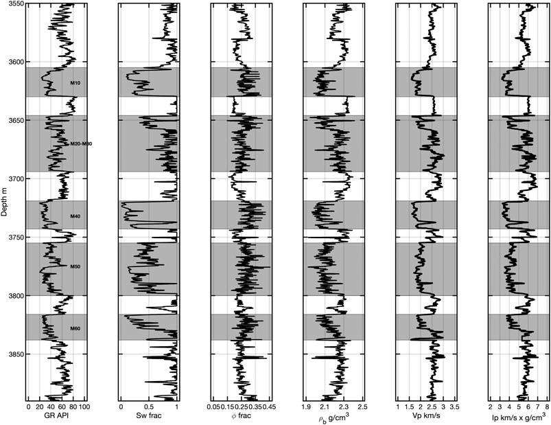
FIGURE 1. Log data from the Gulf of Mexico data set. Included are (A) gamma ray, (B) water saturation, (C) porosity, (D) density, (E) P-wave velocity, and (F) P-impedance. In gray are the M10-M60 sands, also labeled in (A). The sands have lower impedances than the shales and tend to separate cleanly in that domain.
The model selected for this analysis work is the soft-sand model (Dvorkin and Nur, 1996). It has been used with this data set in other publications (e.g., Xie and Spikes,2021). The model is a combination of Hertz-Mindlin (1949) contact theory and modified Hashin-Strikman forms. The Hertz-Mindlin (1949) theory expresses the effective bulk (
and
The terms in Eqs. 1,2 are the Lamé parameters (
Figure 2A contains cross plots of
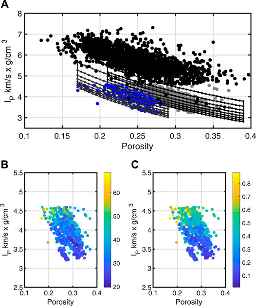
FIGURE 2. Cross plots of P-impedance as a function of porosity. In (A), the black points correspond to shale, gray to oil sands, and blue to gas sands. A series of model lines from the soft sand model are plotted in black for the oil sands and dark gray for the gas sands. The variation in the model lines correspond to porosity in the horizontal direction and water saturation in the vertical. Plots with shading contain only the oil and gas sands color coded by gamma ray (B) and water saturation (C).

TABLE 2. Elastic moduli and densities used in the rock-physics models [modified from Mavko et al. (2009)].
The models plotted in Figure 2A are repeated in Figure 3A without the shale data for clarity. Plots in Figures 2B–D are the same data, but the models have been perturbed relative to those in Figure 3A. In Figure 3B, C changed from 20 to 30%. In Figure 3C, C was changed back to the original, P was reduced from 20 to 15 MPa. Last, the pressure change was removed, and ϕc was changed from 0.36 to 0.35. For simplicity these perturbations were the same for both the gas and oil-sand models. In all four cases, the models qualitatively fit the data, but these fits do not give an indication of which inputs are more significant to change. The Bayesian approach provides a way to assess the significance of the model parameters.
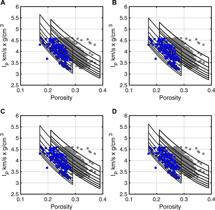
FIGURE 3. The four plots contain perturbed versions of the rock physics models in Figure 2. The oil sands are in gray points and gas sands in blue. The models in (A) are the same as those in Figure 2A. The composition was altered slightly in (B) relative to (A). In (C, D) the pressure and critical porosity, respectively, were changed relative to the models in (A). All four sets of models match the data from a qualitative perspective.
The Bayesian approach includes a quantitative match of model to data. Within it we must compute a prior, p(m), and likelihood function, l (d|m) (i.e., Ulrych et al., 2001; Tarantola, 2005; Sen 2006). The prior (Eq. 3),
is proportional to the exponential that contains differences between the model m and mprior, which is a second and more informed model. Inputs to the rock physics model populate vectors of m and mprior. The differences are scaled by the inverse of the covariance matrix of the prior model, CM.
Next, we define the objective function [
where g(m) is the rock-physics model that calculates simulated values based on the model values in m, d is the real data vector, and the data covariance matrix is represented by CD. The likelihood function (Eq. 5) is then proportional to the negative exponent of the objective function
Last the posterior distribution (
The number of model parameters is four, which is small enough to allow for a tractable analytical solution. No sampling methods are required. We analyze posterior multivariate histograms, so a normalizing factor to obtain probabilities is not needed.
Data input into the analysis is a subset of the oil or gas sands. The selection of the subset is a two-step process. First, one of the rock-physics model lines shown in Figure 2A or Figure 3A is used as a reference. The reference is required because the computed models must be relatively close to the data used in the Bayesian framework. If the data and model are significantly far apart, then the objective function in Eq. 4 has large values, and so the likelihood function (Eq. 5) will have exceedingly small values. Second, data are selected that occur within a certain percent of both
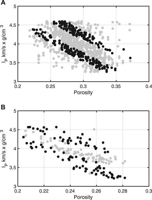
FIGURE 4. (A) Portions of the oil sand data (black points) used in analyses one and two. The lower set corresponds (216 points) to analysis one and the upper (155 points) to analysis two. For the gas sand data (B), the lower set of black points (127 points) corresponds to analysis three and the upper (75 points) to analysis four.
The first set of results comes from analysis 1, for one subset of the oil sands. The model priors are user provided based on some knowledge of the data. The models m and mprior were normal distributions of size 200 × 4, so 200 values of each of the four inputs. Mean values for mprior were [Sw, C, P, ϕc] = [0.4, 0.2, 20, 0.38] and covariance matrix
The mean of m was slightly different, and the covariance matrix for it had slightly larger values on the diagonal. All combinations of the priors were computed, so 2004 models with no sampling. The data to model comparison (Eq. 4) used
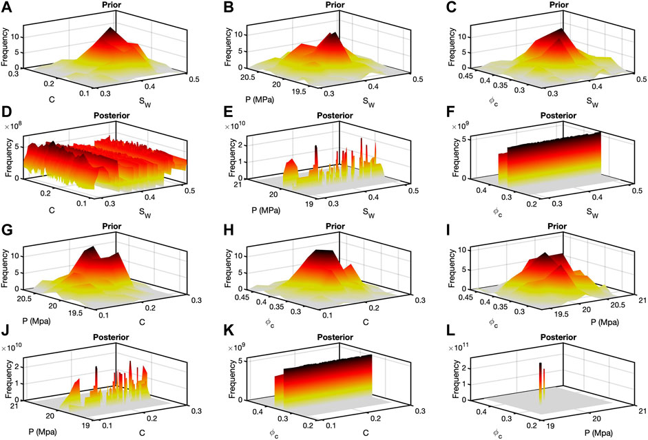
FIGURE 5. Bivariate histograms for analysis one. Plots (A–C) are the bivariate prior histograms for
Figure 6 contains the bivariate priors and posterior histograms for analysis 2, the second oil sand analysis. The procedure for analysis 2 was the same as analysis 1. The only differences were the mean of mprior, which was [Sw, C, P, ϕc] = [0.6, 0.2, 20, 0.38], and the covariance matrix, which was
Similar updates were made for m. The layout of Figure 6 is the same as Figure 5. All six priors are relatively smooth. Four of the six posteriors (Figures 6E,F,J,K) have wide ranges of one parameter with a narrow range of the other. Figure 6D indicates many possible pairs, but the posterior in Figure 6L, like Figure 5L, shows isolated, joint values of ϕc and P.
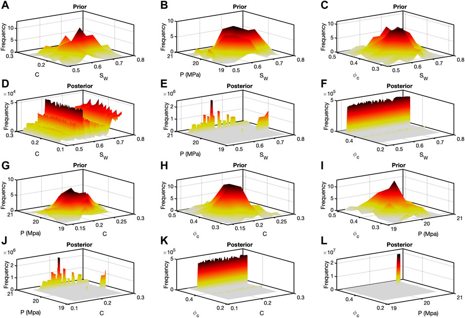
FIGURE 6. Bivariate histograms for analysis two. The juxtaposition is the same as in Figure 5. The prior model differed between analysis one and two, but the bivariate posterior histograms show patterns similar to those in Figure 5.
Results from analyses 3 and 4 are plotted in Figures 7, 8, respectively. The same analysis procedure was repeated again. The means and covariance matrices of the models in analysis 3 were the same as in analysis 1. The difference is that the effective fluid bulk modulus and density is a function of the gas-brine mixture rather the oil-brine mixture. In Figure 7, the posterior histograms resemble the counterparts in Figures 5, 6 although with different peak frequency values. Most notably, the histogram in Figure 7F again shows an isolated joint pair of ϕc and P. Last, in analysis 4, the mean for mprior was [Sw, C, P, ϕc] = [0.72, 0.2, 20, 0.38] and covariance matrix
The bivariate histograms in Figure 8 also resemble their counterparts in Figures 5–7. Figure 8L displays an isolated pair of ϕc and P.
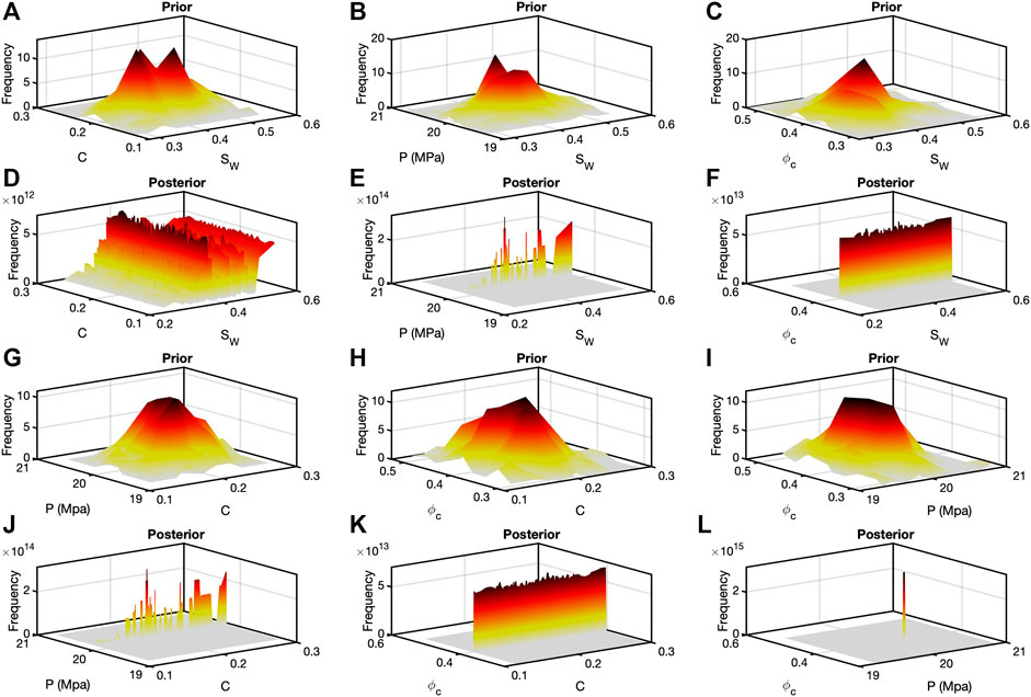
FIGURE 7. Results from anallysis three for gas sands displayed again as bivariate prior and posterior histograms. The layout is identical to Figure 5. The prior was different from inversions one and two including different fluid properties of gas relative to oil. However, the posterior histograms, in particular (D) and (L), resemble their counterparts in Figures 5,6.
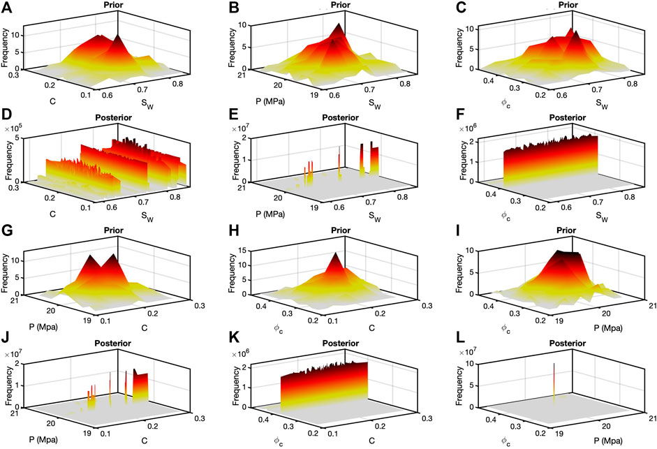
FIGURE 8. Analysis four, for gas sands, resulted in similar bivariate histograms compared with those in Figure 7. However, the frequencies are considerably lower. This is the result of the prior model not being as close to the data as they were in the other inversions. Nonetheless, the patterns repeated themselves among the different posteriors.
The Bayesian analysis method allowed us to determine quantitatively the most and least significant model inputs. Importantly, it revealed correlations between parameters that are not obvious. In all four analyses, the posterior of pressure and critical porosity indicated isolated pairs. Each analysis had a different set of values. If another prior is used, the result would change in terms of the value of pressure and critical porosity, but an isolated set occurs. This correlation is not intuitive, but it indicates that these two parameters are the most significant. Posterior histograms that contain saturation or clay content is more intuitive. More specifically, it is understandable that a small change in either might not change the velocity very much. When one or the other is paired with pressure or critical porosity, the result is a relatively broad range of with a narrow selection of pressure or critical porosity. When applying this method to well data, we considered, fluid types and saturations, and mineralogy along with pressure and critical porosity. Preliminary work indicated similar correlations between pressure and critical porosity on dry, clean sands. The extension to include fluids and composition indicates similar patterns and correlations that were not expected.
This study demonstrates a way to determine the significance of inputs into one rock-physics model. The significance becomes evident of any singular or joint set of rock-physics model parameters. In an application to reservoir characterization, the most significant terms should be set first, and the others can be more loosely defined. If this model was deemed appropriate on a different data set, then in a deterministic application, the most significant inputs should be selected first and jointly. The other inputs would then provide more subtle fine tuning. This approach would limit the number of variables to consider within the requisite sensitivity study for that data set. If this model was used in a statistical seismic inversion, a user could set narrow limits on the priors for the most significant parameters and wider ranges for the lesser ones. The effect of this would be to reduce the size of the model parameter space to explore. This was work done on one model one data set, and the results are relevant specific to this model and applicable to other data sets. Knowledge about this one particular model might be useful for similar types of models, given an appropriate data set, but not likely for other types of models.
The data analyzed in this study is subject to the following licenses/restrictions: Data release contract does not allow of public dissemination of the data used. Requests to access these datasets should be directed to KS, a3lsZS5zcGlrZXNAanNnLnV0ZXhhcy5lZHU=.
KS wrote the codes, the manuscript, and generated the figures MS provided initial motivation for the work, edited the manuscripts, and critiqued the results.
The authors declare that the research was conducted in the absence of any commercial or financial relationships that could be construed as a potential conflict of interest.
Bosch, M., Mukerji, T., and Gonzalez, E. (2010). Seismic inversion for reservoir properties combining statistical rock physics and geostatistics: a review. Geophysics 75 (5), 75A165–75A176. doi:10.1190/1.3478209
Contreras, A. J. (2006). Spatial delineation, fluid-lithology characterization, and petrophysical odeling of deepwater Gulf of Mexico reservoirs through joint AVA deterministic and stochastic inversion of 3D partially-stacked seismic amplitude data and well logs. Doctoral dissertation. Austin, (TX): The University of Texas at Austin.
Dvorkin, J., and Nur, A. (1996). Elasticity of high‐porosity sandstones: theory for two North Sea data sets. Geophysics 61, 1363–1370. doi:10.1190/1.1444059
Grana, D. (2018). Joint facies and reservoir properties inversion. Geophysics 83 (3), M15–M24. doi:10.1190/geo2017-0670.1
Hashin, Z., and Shtrikman, S. (1963). A variational approach to the theory of the elastic behavior of multiphase materials. J. Mech. Phys. Solids 11, 127–140. doi:10.1016/0022-5096(3)90060-7
Mavko, G., Mukerji, T., and Dvorkin, J. (2009). The rock physics handbook. Cambridge, United Kingdom: Cambridge University Press, 254.
Nawaz, M. A., and Curtis, A. (2017). Bayesian inversion of seismic attributes for geological facies using a hidden Markov model. Geophys. J. Int. 208, 1184–1200. doi:10.1093/gji/ggw411
Tarantola, A. (2005). Inverse problem theory and methods for model parameter estimation. Paris, France: Society for Industrial and Applied Mathematics, 352.
Ulrych, T. J., Sacchi, M. D., and Woodbury, A. (2001). A Bayes tour of inversion: a tutorial. Geophysics 66 (1), 55–69. doi:10.1190/1.1444923
Ulvmoen, M., Omre, H., and Buland, A. (2010). Improved resolution in bayesian lithology/fluid inversion from prestack seismic data and well observations: part 2—real case study. Geophysics 75 (2), B73–B82. doi:10.1190/1.3335332
Ulvmoen, M., and Omre, H. (2010). Improved resolution in bayesian lithology/fluid inversion from prestack seismic data and well observations: part1—methodology. Geophys. 75 (2), R21–R35. doi:10.1190/1.3294570
Keywords: rock physics, bayesian analyses, model sensitivity, elastic properties, fluid effect
Citation: Spikes KT and Sen MK (2021) Bayesian Analysis to Determine Relative Significance of Inputs of a Rock-Physics Model. Front. Earth Sci. 9:640698. doi: 10.3389/feart.2021.640698
Received: 11 December 2020; Accepted: 02 February 2021;
Published: 15 March 2021.
Edited by:
Beatriz Quintal, University of Lausanne, SwitzerlandReviewed by:
Priyank Jaiswal, Oklahoma State University, United StatesCopyright © 2021 Spikes and Sen. This is an open-access article distributed under the terms of the Creative Commons Attribution License (CC BY). The use, distribution or reproduction in other forums is permitted, provided the original author(s) and the copyright owner(s) are credited and that the original publication in this journal is cited, in accordance with accepted academic practice. No use, distribution or reproduction is permitted which does not comply with these terms.
*Correspondence: Kyle T. Spikes, a3lsZS5zcGlrZXNAanNnLnV0ZXhhcy5lZHU=
Disclaimer: All claims expressed in this article are solely those of the authors and do not necessarily represent those of their affiliated organizations, or those of the publisher, the editors and the reviewers. Any product that may be evaluated in this article or claim that may be made by its manufacturer is not guaranteed or endorsed by the publisher.
Research integrity at Frontiers

Learn more about the work of our research integrity team to safeguard the quality of each article we publish.