MODIS Does Not Capture the Spatial Heterogeneity of Snow Cover Induced by Solar Radiation

Bouamri, Hafsa; Kinnard, Christophe; Boudhar, Abdelghani; Gascoin, Simon; Hanich, Lahoucine; Chehbouni, Abdelghani

doi:10.3389/feart.2021.640250

ORIGINAL RESEARCH article

Front. Earth Sci., 29 April 2021

Sec. Cryospheric Sciences

Volume 9 - 2021 | https://doi.org/10.3389/feart.2021.640250

This article is part of the Research Topic Climate Impacts on Snowpack Dynamics View all 6 articles

MODIS Does Not Capture the Spatial Heterogeneity of Snow Cover Induced by Solar Radiation

$\r\nHafsa Bouamri$ Hafsa Bouamri¹

Christophe Kinnard^2*

Abdelghani Boudhar^1,3

Simon Gascoin⁴

Lahoucine Hanich^3,5

Abdelghani Chehbouni^3,4

¹Water Resources Management, Valorisation and Remote Sensing Team, Faculty of Sciences and Technology, Sultan Moulay Slimane University, Beni Mellal, Morocco
²Département des Sciences de L’environnement, Centre de Recherche sur les Interactions Bassins Versants – Écosystèmes Aquatiques (RIVE), Université du Québec à Trois-Rivières, Trois-Rivières, QC, Canada
³Center for Remote Sensing Application (CRSA), Mohammed VI Polytechnic University, Ben Guerir, Morocco
⁴CNRS/CNES/IRD/UPS, Centre d’Études Spatiales de la Biosphère (CESBIO), University of Toulouse, Toulouse, France
⁵L3G Laboratory, Earth Sciences Department, Faculty of Sciences and Techniques, Cadi Ayyad University, Marrakech, Morocco

Estimating snowmelt in semi-arid mountain ranges is an important but challenging task, due to the large spatial variability of the snow cover and scarcity of field observations. Adding solar radiation as snowmelt predictor within empirical snow models is often done to account for topographically induced variations in melt rates. This study examines the added value of including different treatments of solar radiation within empirical snowmelt models and benchmarks their performance against MODIS snow cover area (SCA) maps over the 2003-2016 period. Three spatially distributed, enhanced temperature index models that, respectively, include the potential clear-sky direct radiation, the incoming solar radiation and net solar radiation were compared with a classical temperature-index (TI) model to simulate snowmelt, SWE and SCA within the Rheraya basin in the Moroccan High Atlas Range. Enhanced models, particularly that which includes net solar radiation, were found to better explain the observed SCA variability compared to the TI model. However, differences in model performance in simulating basin wide SWE and SCA were small. This occurs because topographically induced variations in melt rates simulated by the enhanced models tend to average out, a situation favored by the rather uniform distribution of slope aspects in the basin. While the enhanced models simulated more heterogeneous snow cover conditions, aggregating the simulated SCA from the 100 m model resolution towards the MODIS resolution (500 m) suppresses key spatial variability related to solar radiation, which attenuates the differences between the TI and the radiative models. Our findings call for caution when using MODIS for calibration and validation of spatially distributed snow models.

Introduction

Snow constitutes a key element in determining water availability in mountainous catchments, especially in arid and semiarid regions, so that a good understanding of snowpack processes is crucial to support water management strategies (Barnett et al., 2005; Viviroli and Weingartner, 2008; De Jong et al., 2009; Vicuña et al., 2011; Mankin et al., 2015; Qin et al., 2020). In this context, modeling snowmelt and snow water equivalent (SWE) at the basin scale represents an important tool for water budget calculation and runoff prediction (Matin and Bourque, 2013; Bair et al., 2016; Fayad et al., 2017; Han et al., 2019).

The lack of ground observations and the large spatiotemporal heterogeneity of snow cover represent challenging limitations for snow studies in remote mountain ranges (Chaponnière et al., 2005; Boudhar et al., 2010, 2016; Rohrer et al., 2013; Marchane et al., 2015; Collados-Lara et al., 2020). In this context, the use of simple conceptual snow models combined with remote sensing data constitutes a useful approach to assess and quantify snowmelt and SWE distribution at the basin scale (e.g., Jain et al., 2010; Abudu et al., 2012; Berezowski et al., 2015; Dozier et al., 2016; Sproles et al., 2016; Steele et al., 2017; Han et al., 2019). Conceptual models use simplified process representations with lower data requirements than physically based models, and are thus widely used for large-scale applications in high mountain catchments where in situ observations are sparse (Singh and Bengtsson, 2003; Schneider et al., 2007; Fassnacht et al., 2017). The most commonly used conceptual snow models are temperature-index models, which depend solely on air temperature to calculate snowmelt using the degree-day method (Hock, 2003). Despite their simplicity, these models can provide reliable estimates of melt rates and perform generally well both at the point scale and within distributed or lumped hydrological models (Vincent, 2002; Abudu et al., 2012; Kampf and Richer, 2014; Senzeba et al., 2015; Hublart et al., 2016; Réveillet et al., 2017). On the other hand, it has been demonstrated that enhanced temperature-index models that include solar radiation as predictor can outperform classical degree-day models (Cazorzi and Dalla Fontana, 1996; Hock, 1999; Pellicciotti et al., 2005; Carenzo et al., 2009; Homan et al., 2011; Carturan et al., 2012; Gabbi et al., 2014; Bouamri et al., 2018). This is to be expected, as solar radiation is one of the main components of the surface energy balance, generally contributing between 50 and 90% of the energy available for melt (Willis et al., 2002; Mazurkiewicz et al., 2008), and has a great influence on the spatial variability of ablation (Herrero et al., 2009; Aguilar et al., 2010; Comola et al., 2015; DeBeer and Pomeroy, 2017).

Representing the spatial variability of snow cover within distributed, parsimonious snowmelt models for hydrological applications remains challenging, especially in mountainous areas where the snow distribution depends on complex relationships between meteorological conditions and the surrounding landscape, primarily topography (Anderton et al., 2004; Molotch et al., 2005; DeBeer and Pomeroy, 2009; Grünewald et al., 2010; Clark et al., 2011). In this sense, various studies have shown that elevation, slope, and aspect play a crucial role in determining the spatial variability of snow processes (Lehning et al., 2006; Letsinger and Olyphant, 2007; López-Moreno and Stähli, 2008). Interactions between topography and solar radiation strongly modulates the shortwave radiation balance and produce considerable shading effects, especially in high relief landscapes (e.g., Olyphant, 1984). While TI models only consider the elevation dependance of temperature to model the heterogeneity of snowmelt rates, adding solar radiation allows to explicitly include the effect of topography on melt and as such to better represent the snow cover heterogeneity (e.g., Cazorzi and Dalla Fontana, 1996; Zaramella et al., 2019). Indeed, previous studies have shown that including solar radiation improved the performance of spatially distributed melt models for predictions of glacier mass balance (Gabbi et al., 2014), snow cover area (Cazorzi and Dalla Fontana, 1996; Follum et al., 2015), and streamflow from snow-fed basins (Brubaker et al., 1996; Follum et al., 2019; Massmann, 2019). Given the larger computational cost entailed to calculate spatially distributed radiation maps, it is important to assess their relevance for estimating snowmelt with conceptual models aimed for operational hydrological applications.

Including solar radiation in distributed snowmelt models raises the question about the appropriate scale (resolution) to run models and the suitability of available data to validate them (Baba et al., 2019). While distributed empirical models can be run at high spatial resolutions (<1 km) over large catchments (>1000 km²), few observations are usually available to validate spatial simulations explicitly. Snow depth maps from repeat lidar surveys (Bair et al., 2016; Painter et al., 2016) and satellite photogrammetry (Marti et al., 2016) are becoming increasingly available, but they remain rare, so that snow cover area (SCA) maps often represent the sole source of spatially distributed snow information to validate distributed snow models. Snow cover maps derived from the Moderate-Resolution Imaging Spectroradiometer (MODIS) sensor onboard the Terra and Aqua satellites, available since 2000 and 2002, respectively, have been at the forefront of distributed snow model calibration and validation efforts (Parajka and Blöschl, 2008; Finger et al., 2011; Franz and Karsten, 2013; Gascoin et al., 2013; Duethmann et al., 2014; He et al., 2014; Baba et al., 2018). However, its spatial resolution (~500 m) may often be larger than the resolution of key processes, such as topographic radiation loading and snow drifting.

This paper examines how temperature index snowmelt models enhanced with different solar radiation components impact the simulated spatiotemporal variability of SWE and snowmelt, and investigates scaling issues arising when using MODIS snow cover area maps for model validation. We specifically aim to show (i) how solar radiation impacts the simulated snowmelt dynamics and resulting spatiotemporal heterogeneity in snow cover area, and (ii) if and how this heterogeneity is captured by MODIS snow cover area products that are commonly used for model calibration and validation. This question has not yet been explored in the snow hydrology community and should thus provide further guidance for the implementation and validation of distributed empirical snow models.

Study Area

The study was carried out in the Rheraya headwater watershed in the High Atlas Range in central Morocco (Figure 1). Snowmelt in this region has important socio-economic implications by providing fresh water to irrigate the arid plains downstream, supplying drinking water for populations and supporting hydropower generation (Chehbouni et al., 2008). The watershed covers an area of 228 km², and its elevation ranges from 1060 m a.s.l to the Jbel Toubkal summit at 4167 m a.s.l., the highest summit of North Africa. Slopes in the basins are steep (mean of ~24° from a 100 m resolution DEM) and characterized by sparse vegetation in the spring which quickly disappears in summer due to aridity. The Rheraya watershed has a mixed snow-rain regime and constitutes the most important water supply for the downstream region (Schulz and de Jong, 2004; Chaponnière et al., 2005; Rochdane et al., 2012; Hajhouji et al., 2018). Average annual precipitation was 520 mm from 1988 to 2010 as measured at the Club Alpin Francais (CAF) station at 2612 m above sea level (a.s.l), where 50% occurred as snow during winter months (Boudhar et al., 2016). The snow cover is highly variable at annual and inter-annual time scales and the snowmelt was found to contribute from 28 to 48% of the annual river discharge (Boudhar et al., 2009). The Rheraya has been used as an experimental site for mountain hydrological studies in the Tensift River basin (Jarlan et al., 2015), leading to a concentration of studies on snow and hydrology in this basin (Boudhar et al., 2016; Baba et al., 2018, 2019; Bouamri et al., 2018; Hajhouji et al., 2018).

FIGURE 1

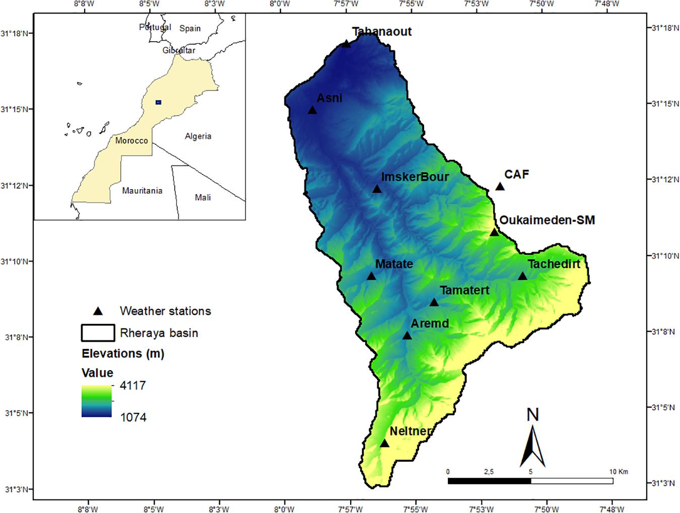
Figure 1. Geographical location of the Rheraya basin and weather stations.

Data and Methods

The different datasets used in this study are summarized in Table 1 and detailed in the following sub-sections.

TABLE 1

Table 1. Data used in the current study.

Digital Elevation Model

A 4 m spatial resolution Digital Elevation Model (DEM) derived from Pleiades stereoscopic imagery was used to represent the basin topography. Details about DEM processing are provided in Baba et al. (2019). The DEM was previously validated for the Rheraya catchment, showing a vertical absolute accuracy of 4.72 m (Baba et al., 2019). The DEM was aggregated to a coarser 100 m resolution using bilinear resampling. This resolution was chosen as a good tradeoff allowing for a reasonable model computation time while adequately representing the dominant topographic features in the Rheraya catchment (Baba et al., 2019).

Meteorological Forcing Data

Daily meteorological data obtained from ten stations at various locations within or near the Rheraya watershed were used to distribute meteorological variables to the catchment area (Figure 1 and Supplementary Table 1). While precipitation measurements were available at all ten stations, the availability of air temperature and relative humidity varied among stations and over time (Supplementary Figure 1). Two high elevation stations, Oukaimeden-SM (3230 m a.s.l.) and Neltner (3207 m a.s.l.) have unheated rain gauges, so their precipitation records were excluded to avoid interpolating unreliable observations in winter. The CAF station (2612 m a.s.l.) is thus the only high elevation station with reliable precipitation observations since rainfall and snowfall are independently and manually measured since 1988 (Figure 1).

Satellite Data

MODIS Daily Snow Product

Snow cover maps were derived from the Moderate Resolution Imaging Spectroradiometer (MODIS) daily snow cover products MOD10A1 and MYD10A1 (MODIS Snow Cover Daily L3 Global 500 m SIN GRID V006), respectively, generated from the Terra and Aqua MODIS satellites, and acquired from the National Snow and Ice Data Center (NSIDC) (Hall and Riggs, 2016). The MODIS snow products from the Terra and Aqua satellites are available since February 2000 and February 2002, respectively. The datasets are produced in a Geographic projection and were re-projected to the World Geodetic System 1984 (WGS84) Universal Transverse Mercator (UTM) coordinate system using the data transformation options available at NSIDC. A total of 4734 MOD10A1 images and 4760 MYD10A1 images, covering 13 years from September 2003 to August 2016, were used in this study. Snow cover was identified using the Normalized Difference Snow Index (NDSI), which captures the high contrast between the characteristically high reflectance of snow in the visible spectrum and its low reflectance in the shortwave infrared spectrum (Hall et al., 1995). Starting in MODIS version 6, the fractional snow cover (FSC) has been replaced by the NDSI which is designed to detect snow cover with high accuracy over a wide range of viewing conditions, besides providing more flexible data to the user (Riggs et al., 2015).

Processing and Combining MOD10A1 and MYD10A1

Cloud obscuration is the main obstacle to using MODIS snow cover products (Parajka and Blöschl, 2008; Xie et al., 2009; Zhou et al., 2013). The Terra and Aqua satellites have an approximate 3 h average overpass time difference, during which cloud conditions can change significantly (Xue et al., 2014). Various previous studies have shown that combining Terra and Aqua observations reduces cloud obscuration (Parajka and Blöschl, 2008; Gafurov and Bárdossy, 2009; Wang and Xie, 2009; Xie et al., 2009; Gascoin et al., 2015). For example, Gao et al. (2010) reported that combining Terra and Aqua improved cloud filtering by reducing the influence of transient clouds in daily reflectance data by 11.7% compared to using MOD10A1 alone, and by 7.7% compared to using MYD10A1 alone. In this study, the MOD10A1 and MYD10A1 were merged into a combined product called CMXD10A (Figure 2) as follow: (i) on any given day if only one source (either Terra or Aqua) was available it was used for that day; (ii) for days when both products are available, priority was given to the Terra product (e.g., Xie et al., 2009) since the Aqua MODIS instrument provides less accurate snow maps due to dysfunction of band 6 on Aqua (Riggs and Hall, 2004; Salomonson and Appel, 2006; Gascoin et al., 2015; Zhang et al., 2019). This means than any pixel classified as either cloud, missing, or unclassified in MOD10A1 was filled with the corresponding pixel in MYD10A1 if that pixel had a NDSI value, else the original MOD10A1 pixel classification was conserved (Figure 2). Subsequently, a spatiotemporal filter was applied to the merged CMXD10A product to fill in missing NDSI data, i.e., pixels classified as cloud, but also those classified as either missing, saturated or unclassified, collectively referred to as ‘missing’ therein. A spatial filter was first applied only if less than 60% of the mountainous areas (elevations above 1000 m) were missing (Marchane et al., 2015). This filter classifies missing pixels as being fully snow-covered (NDSI = 1) when their elevations is higher than the average elevation of other fully snow-covered pixels in the entire basin. Then, a temporal filter was applied to linearly interpolate the remaining missing pixels within a moving window extending 3 days prior and 2 days after the current date. This time window was previously shown to be efficient for cloud gap filling by Marchane et al. (2015) in the Rheraya catchment. NDSI values in the blended and interpolated CMXD10A product were converted to binary maps of snow cover area (SCA) based on an NDSI threshold of 0.4, following previous studies (Xiao et al., 2004; Marchane et al., 2015; Hall and Riggs, 2016), i.e., for each pixel, SCA = 1 when NDSI ≥ 0.4, otherwise SCA = 0 (Figure 2). The number of pixel identified as missing over the entire period was reduced from 22.35% in MOD10A1 to 0.84% after blending both MODIS products and applying cloud interpolation, which is similar to previous results obtained in the same area by Marchane et al. (2015).

FIGURE 2

Figure 2. Flowchart describing the steps for processing MODIS data and comparing MODIS and simulated snow cover area (SCA). Purple color, data source; pink, intermediate output; gray, main output.

Snowmelt Models

Four different melt models were used to simulate snowmelt and SWE in the Rheraya watershed. The benchmark model is a classical degree-day or ‘temperature index’ (TI) model (Hock, 2003), which uses air temperature as the sole predictor for melt. This model was ‘enhanced’ with different solar radiation terms: (i) Hock’s temperature index melt model (HTI) which includes clear sky potential solar radiation (Hock, 1999); (ii) an enhanced temperature-index (ETIA) including global radiation and (iii) an enhanced temperature-index (ETIB) that includes albedo (Pellicciotti et al., 2005; Table 2). These models were previously calibrated and validated at the point scale at the Oukaimeden-SM weather station site (Bouamri et al., 2018), and the same model coefficients were used for the spatial simulations in this study (Table 3). Further model descriptions and results regarding model performances at the point scale are presented in detail in Bouamri et al. (2018), and only the main model equations are given in Table 2.

TABLE 2

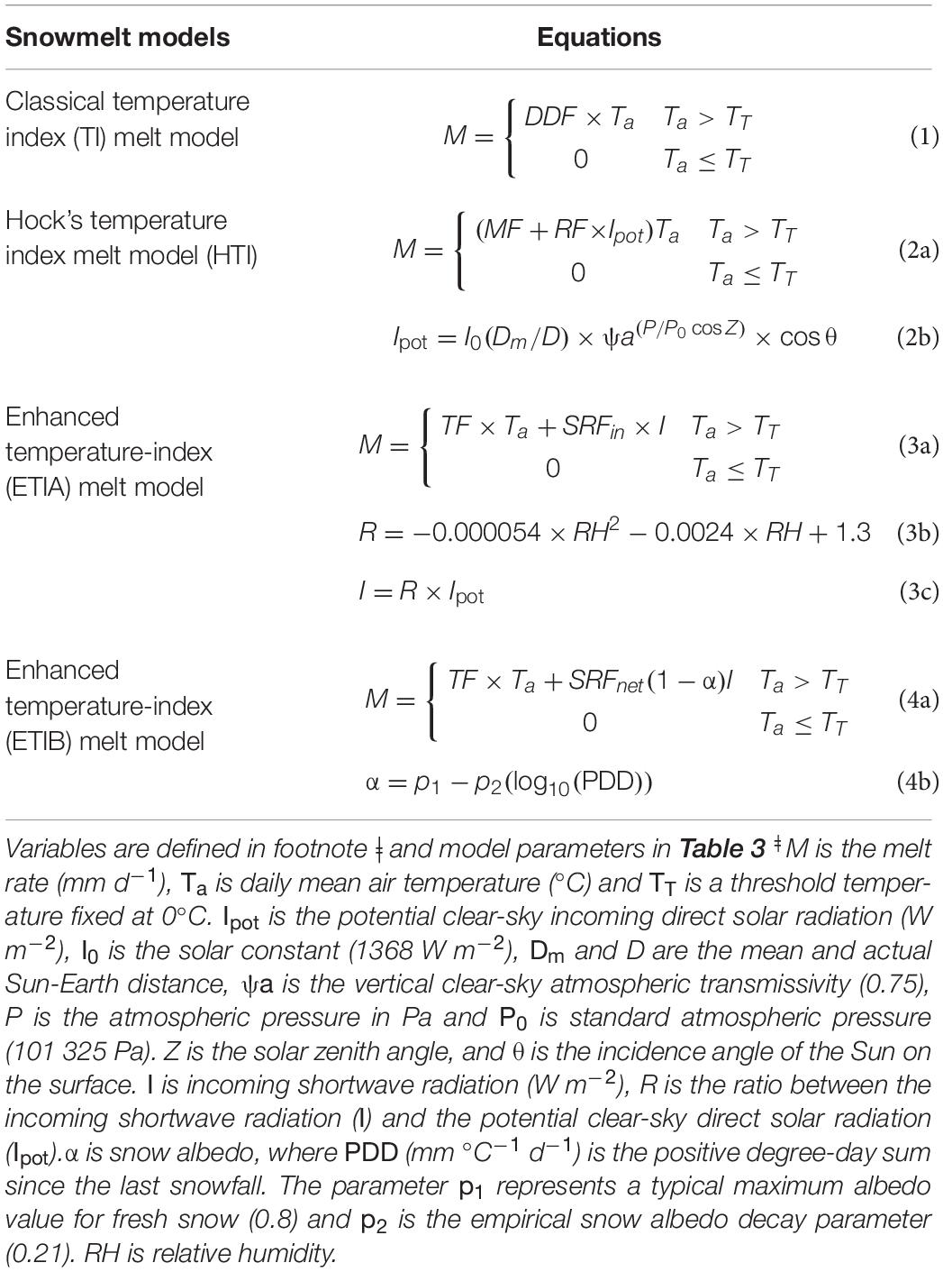
Table 2. Melt models equations used in this study.

TABLE 3

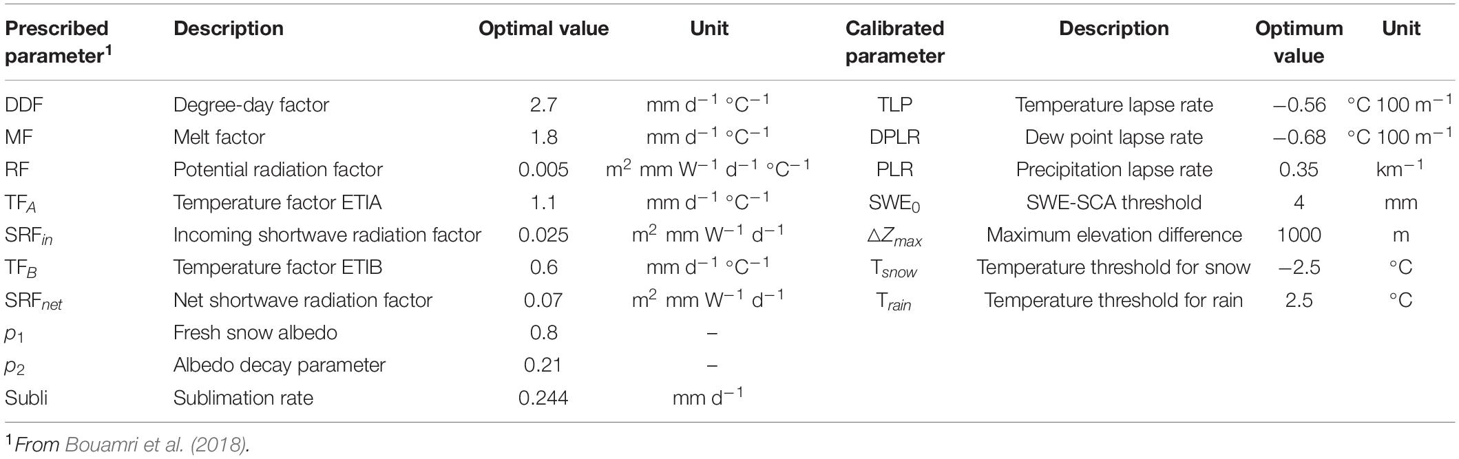
Table 3. Summary of prescribed and calibrated model parameters.

Sublimation losses are not accounted for in empirical melt models. These can be significant in the Rheraya basin, representing 7–20 % of annual snowfall (Boudhar et al., 2016). To take into account sublimation losses, a constant average mean daily sublimation rates was used over the entire basin (Table 3), based on the energy balance study at the Oukaimeden-SM site by Boudhar et al. (2016). While this approach is admittedly simple, it allows correcting for first order sublimation losses (Jost et al., 2012) and as such avoid compensating these losses by artificially reducing precipitation during spatial interpolation and/or overestimating melt, as can be the case when sublimation losses are completely ignored.

Rain/Snow Partition

Determination of the precipitation phase has a large influence on hydrological modeling in mountain areas (Yasutomi et al., 2011; Marks et al., 2013). A linear transition technique was used for the rain-snow partition (e.g., Marks et al., 2013; Feiccabrino et al., 2015). The snowfall fraction is linearly interpolated between a temperature threshold for rain T_rain(°C), and a temperature threshold for snow T_snow (°C) (Tarboton and Luce, 1996; Moore et al., 2012). The daily snowfall (SF) and rainfall (RF) are computed as:

S F = P_{x} (T_{r a i n} - T_{x}) / (T_{r a i n} - T_{s n o w}) (1a)

R F = P_{x} - S F (1b)

Where P_x is total precipitation and T_x is air temperature at gridpoint x. If the daily air temperature is above the T_rain threshold then RF = P_x and SF = 0, while if T_x < T_snow then RF = 0 and SF = P_x. The two fixed temperature thresholds, T_rain and T_snow, were calibrated on odd years and validated on even years using independant observations of snowfall and rainfall available at the CAF station over 2003–2016. Optimal values for T_snow and T_rain were -2.5 °C and 2.5 °C, respectively. The agreement between simulated and measured precipitation was fair for rainfall, with a Nash-Sutcliffe Efficiency score (NSE) (Nash and Sutcliffe, 1970) of 0.54 and correlation coefficient (r) of 0.75, and better for snowfall (NSE = 0.77, r = 0.88) (Supplementary Figure 3). The better performance for snowfall is encouraging for the ensuing SWE modeling.

Spatialization of Meteorological Forcing

Half-hourly meteorological observations retrieved from the different weather stations were averaged to daily interval for the entire study period (2003–2016). Relative humidity (RH) was converted to dew point temperature (DP) following Liston and Elder (2006), since RH is considered a non-linear function of elevation. Mean monthly lapse rates (i.e., averaged over the whole period) were determined by linear regression of air temperature (Ta) and DP against elevation. Since the seasonal variability in the lapse rates was small, a mean annual value was used in the models (Table 3). To distribute Ta and DP observations, station observations were first adjusted to a common elevation using the calculated lapse rate for each variable, and then spatially interpolated to the entire basin using the Barnes objective analysis scheme, following Liston and Elder (2006). The Barnes scheme is used for interpolating data from irregularly spaced observations to a regular grid using a two-pass scheme (Barnes, 1964). The interpolated values are then lapsed back to their original grid elevation using the same lapse rate, and the DP reconverted to RH.

Precipitation was spatially distributed by combining spatial interpolation with a non-linear lapse rate, following Liston and Elder (2006). First, precipitation observations are interpolated to the model grid using the Barnes objective analysis scheme. A reference topographic surface is constructed by interpolating the station true elevations (as measured by GPS) using the same method. The modeled precipitation rate P_x (mm d^–1), at a grid point x with elevation Z_x is computed as:

P_{x} = P_{0} \times \frac{[1 + P L R (Z_{x} - Z_{0})]}{[1 - P L R (Z_{x} - Z_{0})]} (2)

Where P₀ is the interpolated station precipitation, Z_0 is the interpolated station elevation, and PLR (mm km^–1) is the precipitation lapse rate, or ‘correction factor’ (Liston and Elder, 2006). An interpolated topographic reference surface (Z_x) is used rather than a fixed reference because the precipitation adjustment function (equation (2)) is a non-linear function of elevation (Liston and Elder, 2006).

Due to the large spatial and temporal heterogeneity of observed precipitation in Rheraya, a specific calibration of PLR was sought. A range of 0.21- 0.35 km^–1 was used based on the lapse rate value fitted to station observations and the typical winter value set by Liston and Elder (2006) and also found by Baba et al. (2019) in the Rheraya basin. The PLR was calibrated against positive SWE changes at the Oukaimeden-SM station, a proxy for snow accumulation, over a lumped 3-year period (2003-2006) and validated separately on the remaining 2 years (2007–2008, 2009–2010) (Supplementary Figure 2). The optimal value found, 0.35 km^–1, was used to distribute precipitation using equation (2).

The extrapolation of precipitation using equation (2) can result in unrealistically large accumulation rates at high elevations where there are few stations to constrain precipitation. Several studies have shown that while precipitation typically increases with elevation in mountain basins due to orographic uplifting of air masses, this increase can cease and precipitation even decrease passed a certain elevation (Alpert, 1986; Roe and Baker, 2006; Eeckman et al., 2017; Collados-Lara et al., 2018). This is caused by the progressive depletion of moisture available for condensation within the rising air mass. As such, it is crucial in hydrological modeling to limit the vertical extrapolation of precipitation to avoid artificial snow build up at high elevations (Freudiger et al., 2017). In this sense, Liston and Elder (2006) limited the difference between the actual (Z_x) and interpolated (Z_0) station elevation (△Z=Z_x-Z₀) to a default maximum value (△Z_max) of 1800 m. Since there are no stations with reliable precipitation data above the CAF station (2612 m) to constrain this value, this parameter was subjected to a calibration/validation procedure against the MODIS SCA maps for all melt models. △Z_max was calibrated on odd years within a 300-1800 m range and validated on even years for each model in order to reduce the climate dependency of the calibration period (Arsenault et al., 2018). The validation was done using the optimal parameter for each model as well as with the mean of the optimal parameters of each model (mean △Z_max).

The potential, clear-sky direct solar radiation was calculated as a function of solar geometry, topography and a constant vertical atmospheric transmissivity following Hock (1999), and includes topographic shading (Equation 4b in Table 2). Global radiation is calculated using a cloud factor parameterization based on relative humidity (Bouamri et al., 2018) (Equation 5b, c in Table 2) and the net radiation uses an albedo parameterisation based on accumulated positive degree days (Brock et al., 2000) (Equation 6b in Table 2). Further details are given in Bouamri et al. (2018).

Model Validation

The daily snow cover area (SCA) from the merged CMXD10A product was used to assess the ability of each model to simulate the spatiotemporal variability of snow cover in the Rheraya basin over the 2013-2016 period. A conversion of the simulated SWE to SCA was required to compare the simulated SCA with MODIS SCA. This conversion was performed using a constant threshold (SWE₀), i.e., for each grid, SCA = 1 when SWE ≥ SWE₀ and SCA = 0 otherwise. The conversion was done at the model resolution (100 m). The use of this fixed threshold avoids more complex snow depletion curves that require more parameters unknown in our area (Magand et al., 2014; Pimentel et al., 2017). Therefore, SWE₀ was subjected to the same calibration/validation procedure as for△Z_max, using a range of values from 1 to 20 mm following previous studies (Gascoin et al., 2015; Baba et al., 2019).

Confusion matrices were used to assess the classification accuracy of the simulated SCA maps relative to MODIS SCA. Confusion matrices are two-dimensional contingency tables that display the discrete joint distribution of simulated and observed data frequencies (Zappa, 2008). Model skill scores were derived from the confusion matrix (Table 4). The Heidke Skill Score (HSS) (Heidke, 1926) which is equivalent to the Kappa coefficient proposed by Cohen (1960), measures the classification accuracy relative to that expected by chance and has been extensively used for imbalanced datasets such as snow remote-sensing data (e.g., Zappa, 2008; Notarnicola et al., 2013; Baba et al., 2019). The HSS was thus the preferred global metrics used for model assessment. Still, because no global metric is able to completely depict the types of classification errors committed by a model, four metrics based on marginal ratios of the confusion matrix were also used to investigate model errors, as done in several previous studies (e.g., Parajka and Blöschl, 2012; Rittger et al., 2013; Zhou et al., 2013; Zhang et al., 2019). The true positive rate (TPR) measures the proportion of MODIS snow-covered pixels correctly identified as such by the model. Oppositely, the true negative rate (TNR) measures the proportion of MODIS snow-free pixels correctly simulated by the model. The false-negative rate (FNR) measures the proportion of MODIS snow-covered pixels incorrectly identified as snow-free by the model. Complementarily, the false-positive rate (FPR) or ‘False Alarm Rate’ (FAR) as called by Zappa (2008) is the proportion of MODIS snow-free pixels incorrectly identified as snow-covered by the model. Further descriptions of theses metrics are given in Table 4.

TABLE 4

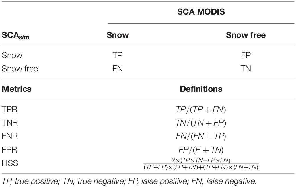
Table 4. Description of confusion matrix between simulated and MODIS SCA, and the evaluation metrics used for model assessment.

Results

Basin-Wide Snow Cover Area

Parameter Sensitivity and Calibration

The sensitivity of SCA model performance to the maximum elevation difference (△Z_max) and SWE-SCA conversion threshold (SWE₀) was assessed using the mean daily HSS metric computed over the calibration period, i.e., the odd years of the 2003-2016 period (Figure 3). Generally, the model performance increases with model complexity, i.e., the HSS is lowest for TI and highest for ETIB. All four models are more sensitive to △Z_max than the SWE₀ parameter. The mean optimal SWE₀varies between 3 mm for TI to 6 mm for ETIB, with little variations in HSS score within this range as well as within each model. A mean optimal SWE₀ value of 4 mm was thus used for validation on even years and for further inter-model comparisons. This value is small compared to the 40 mm threshold used by Baba et al. (2019) and Gascoin et al. (2015) but SWE₀ is resolution dependent, increasing with pixel resolution (Gascoin et al., 2019). The optimal △Z_max shows more variability between models, increasing with model complexity, i.e., lowest for TI and highest for ETIB. This is in fact to be expected from this parameter, which should also partly correct errors in modeled ablation. Using a common △Z_max and SWE₀ value avoids the problem of compensating snowmelt parameterisation errors in each model, which would prevent any further direct comparison of the snowmelt parameterisations. A mean △Z_maxof 1000 m, which is within the zone of maximum performance for each model (Figure 3) was thus used for validation across models and for further inter-model comparisons. Choosing the multi-model average parameter set (SWE₀ = 4 mm, △Z_max 1000 m) over the model-specific optimal parameters affects little the performance in validation (Figure 3). In fact, a slight increase in performance is even noted for ETIB, which suggests that the model-specific values may be slightly overfitted and less transferable compared to the multi-model average parameter set.

FIGURE 3

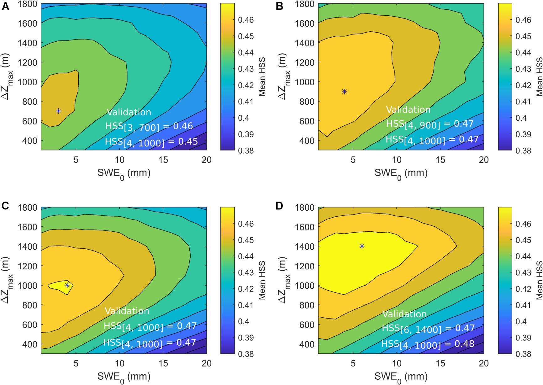
Figure 3. Sensitivity of model SCA simulation performance, as assessed with the mean HSS index, to △Z_max and SWE₀parameters over the calibration period. Optimal parameter values are indicated by asterisks (*). The validation HSS statistics for the model-specific and multi-model average optimal parameters are shown in white. (A) TI, (B) HTI, (C) ETIA, and (D) ETIB.

The slight overall differences in performance between models suggest that, on average, all models have similar abilities to classify snow vs. snow free MODIS pixels, as assessed by the mean HSS metric. The small differences could be partly attributed to the fact that performance metrics are averaged over the whole calibration period. Hence, interannual and seasonal differences in model performance are investigated next.

Basin-Wide SWE and SCA

Time series of daily simulated basin wide SWE and fractional snow cover (fSCA) show significant intra and inter-annual variability over the period (2003-2016) (Figure 4). The fSCA simulated by the four models are in good agreement overall with MODIS observations, both in terms of timing and magnitude. In some years, however, the simulated snow cover lasts longer than observed in MODIS (2004, 2005, 2007, 2008, 2009, and 2012). Those years had above average basin-wide simulated SWE (Figure 4A), so that overestimated accumulation in the upper basin during these wetter years could be the cause for the longer-lasting simulated SCA (Figure 4C). In contrast, in years with scarce snowfall and thinner simulated snowpack (e.g., 2011, 2013, 2014, and 2016), the agreement between simulated and observed fSCA is better (Figure 4D). The varying availability of precipitation records over time could also partly explain this pattern (Supplementary Figure 1).

FIGURE 4

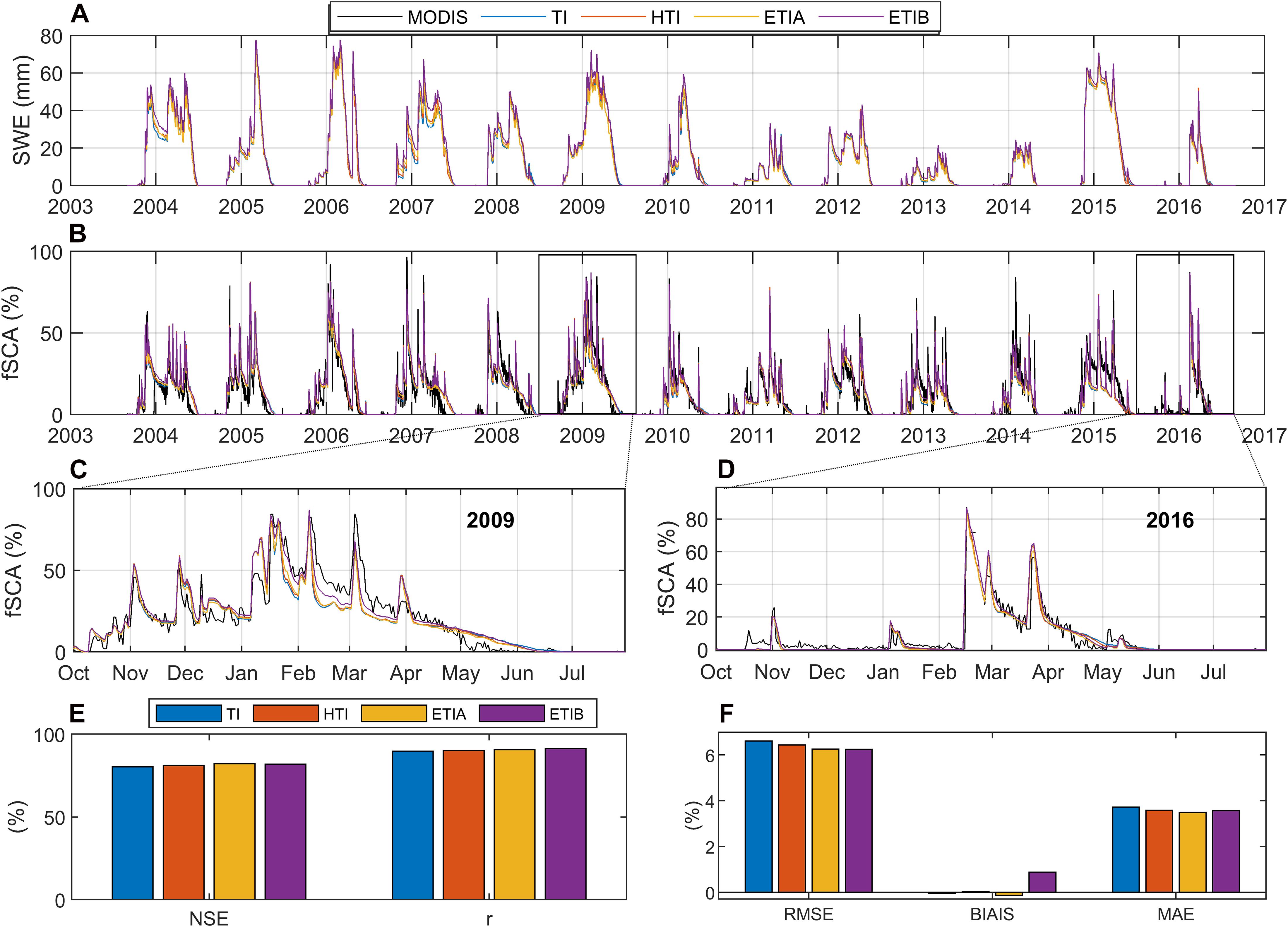
Figure 4. Time series of (A) simulated mean snow water equivalent (SWE), and (B) simulated mean fractional snow cover area (fSCA) of all models vs. MODIS; (C) zoom in on 2009 year; (D) zoom in on year 2016; (E,F) errors statistics over the entire period 2003–2016 in the Rheraya catchment.

All four models show slight differences in their basin-wide fSCA and SWE predictions. Error metrics for the whole period (2003-2016) show that increasing model complexity slightly improves the correlation (r) and predictive skill (NSE) for basin-wide fSCA (Figure 4E). Both the root mean squared error (RMSE) and mean absolute error (MAE) also decrease with model complexity, but a larger bias for the ETIB model slightly increases its MAE relative to the ETIA model (Figure 4F). Hence, overall, the best performance is primarily observed for both enhanced radiative models ETIA and ETIB followed by the HTI and the classical TI models. Still, given the slight differences between models and the increased computational cost associated with enhanced radiative models, the TI model offers at first glance a satisfactory performance to simulate SWE for hydrological applications in the High Atlas range. The causes for inter-model differences in model performance and in simulated SWE and melt are explored in the next sections.

Seasonality

The seasonality of the simulated SWE and fSCA was investigated to better understand seasonal inter-model differences (Figures 5A–C). The enhanced models were then contrasted with the reference TI model to highlight the effect of the different radiation terms on the simulated snow cover (Figures 5D,E). The mean basin SWE seasonal cycle calculated over snow-covered areas (‘SCA SWE’) shows similar variations among models, particularly during the accumulation season (October-March) (Figure 5A). The mean simulated peak occurs in April and varies from 172 mm to 195 mm between models. Increasing differences between the ETI models and TI from March to May reflect the increasing ablation rates simulated by these models relative to TI, while the HTI model differs significantly from TI only from May onward when the SCA is low (Figure 5D). Maximum differences with TI are reached at peak SWE in April for ETIA (-24 mm) and ETIB (-14 mm) and in June for HTI (-21 mm) (Figure 5D). The ETIA model, which does not include albedo feedbacks, thus tends to accentuate most the melt rates in early spring compared to TI. The melt coefficients of ETIA, previously calibrated at the Oukaimeden station, may be slightly biased towards late spring conditions, which results in exaggerated late-winter/early spring melt rates (Bouamri et al., 2018).

FIGURE 5

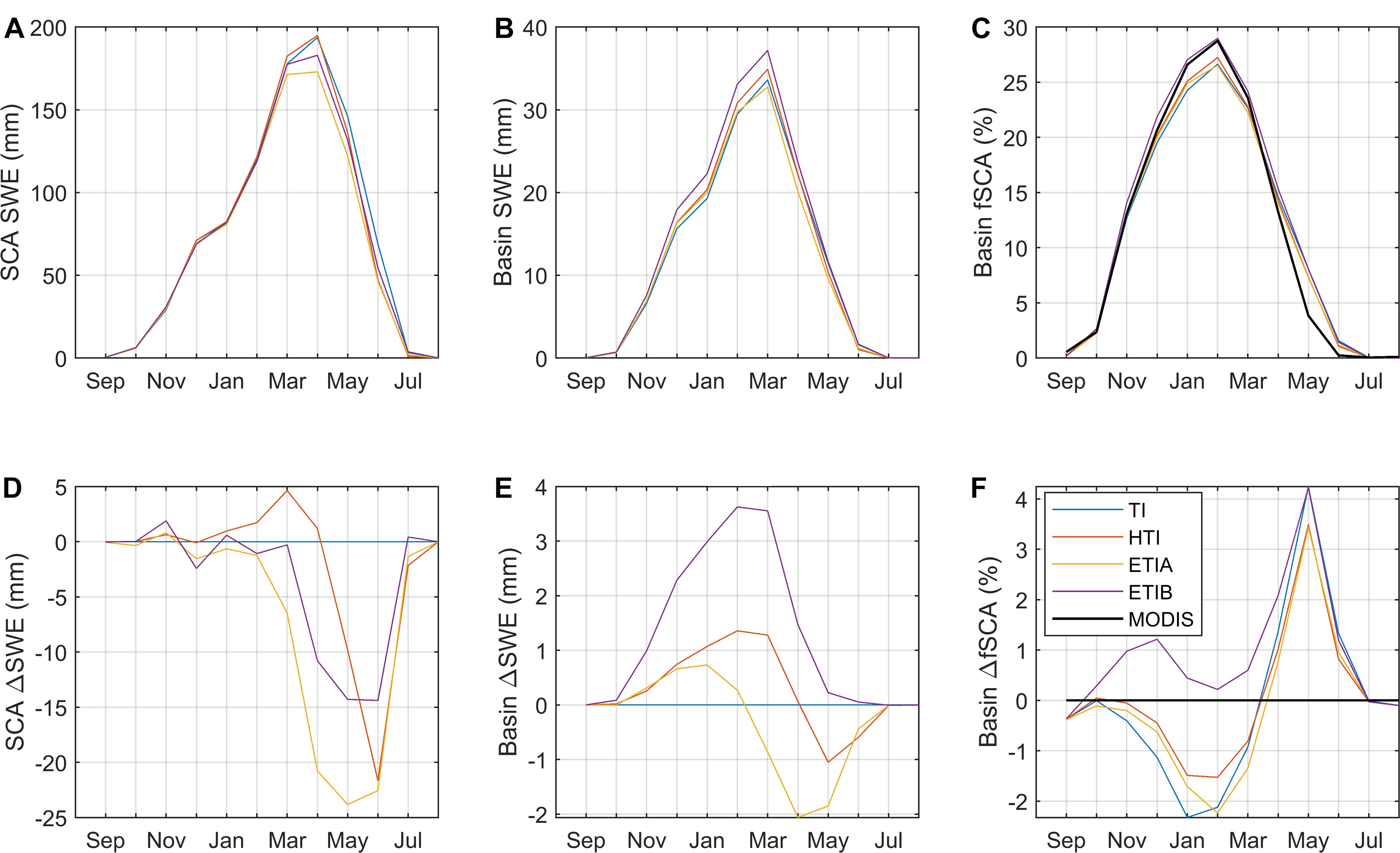
Figure 5. Seasonal cycle of mean simulated snow water equivalent (SWE). (A) Over snow-covered area only. (B) Over the whole basin. (C) Mean simulated fSCA vs. MODIS. (D,E) Difference between radiative models and the reference TI model for panels A and B. (F) Difference between modeled and MODIS fSCA.

When considering mean SWE over the whole basin surface (“Basin SWE”), differences between the enhanced models and TI are more positive during winter and occur at different times (Figure 5B). ETIB stands out with the largest mean peak SWE of 37 mm in March, followed by HTI and the other models. In contrast to the classical TI model, all radiative models simulate higher mean basin SWE during the accumulation period, while ETIA and HTI simulate lower SWE in late spring compared to TI.

The different seasonal behaviors for the mean basin SWE and mean SWE over snow covered areas can be explained by differences in simulated SCA. All models, except ETIB, underestimated MODIS fSCA during accumulation, whereas all models overestimated MODIS fSCA on average during the ablation period, by up to 4.2% for ETIB and TI, and by 3.4% for HTI and ETIA (Figures 5C,F). This confirms the tendency identified in Figure 4 for wet years to have a longer-lasting snow cover simulated by all models, relative to MODIS. Inter-model differences show that all enhanced models simulate a larger snow cover than TI during the accumulation period, with ETIB being the most different and also most in line with MODIS, followed by HTI and ETIA. This explains the positive differences in basin SWE between these models and TI during the accumulation period (Figures 5B,E).

Seasonal variations in SCA model performance, as measured by the HSS index, were investigated over the whole period (Figure 6). Globally, the HSS metric is highest (~0.6-0.75) during winter and spring (December-April) but decreases sharply during the shoulder seasons (October to November and May to June). This shows that the model performance is generally good during most of the snow season, but that classification errors increase when the snow cover is more restricted in the basin. All radiative models performed better than TI especially in the accumulation period, with ETIB performing best, with a maximum increase in HSS of 0.03. The models become gradually more similar in late spring (May-June).

FIGURE 6

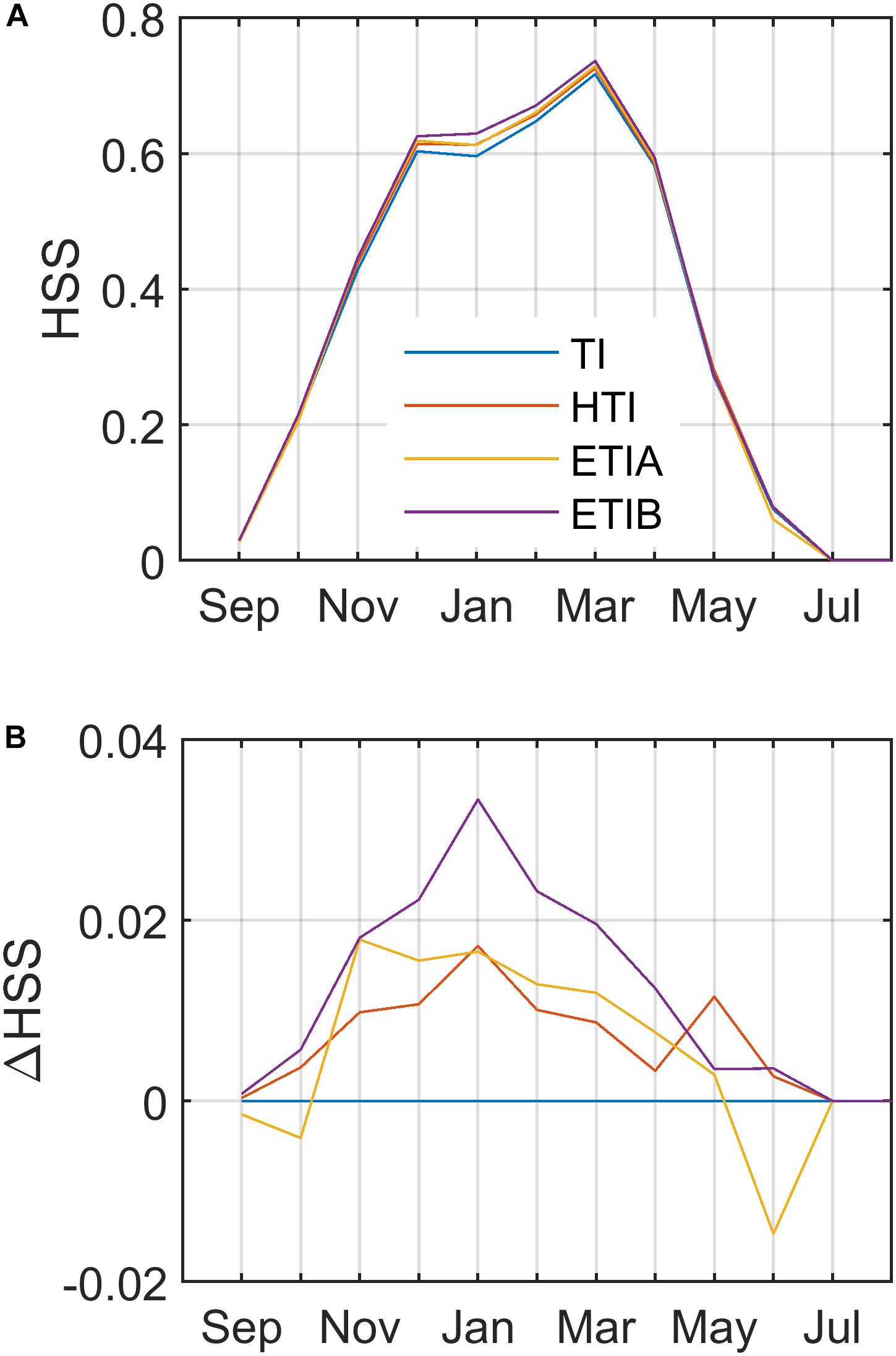
Figure 6. Seasonal model performance. (A) Mean seasonal cycle of HSS index over the whole 2003–2016 period. (B) Differences between enhanced radiative models and the reference temperature index (TI) model.

Spatial Variability

Model performance in predicting spatial variations in SCA was investigated by plotting the HSS metric by elevation bins (Figure 7). Overall, the HSS index increases with elevation for all models (Figure 7B). The mean simulated fractional snow cover area (fSCA) also increases with elevation, in line with MODIS fSCA, but all models start overestimating fSCA above 3500 m (Figure 7A). The worst model performance (lowest HSS) are thus associated with the marginal and transient snow conditions found at the lowest elevations of the basin. Since these elevation areas represent a large share of the basin hypsometry (Figure 7A), the higher classification errors in these areas have a large influence on the basin-wide and time-averaged performance metrics, as displayed on Figure 3.

FIGURE 7

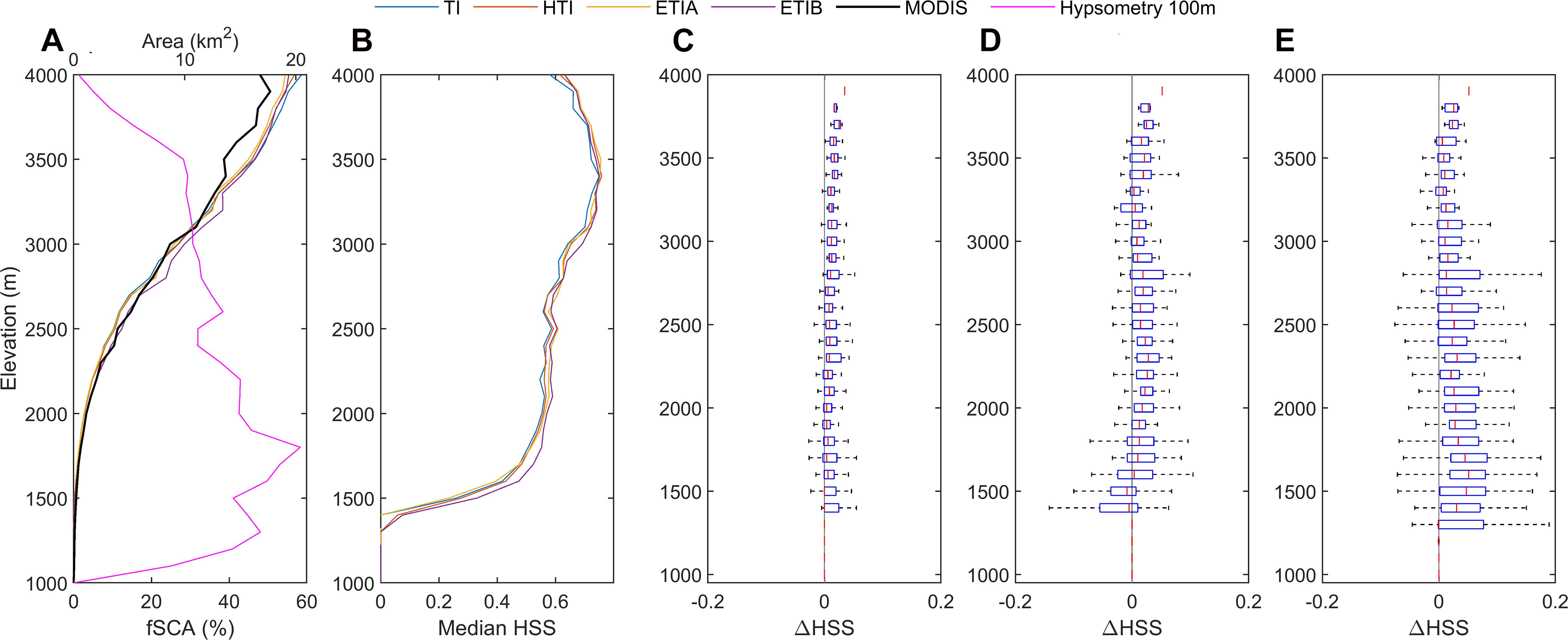
Figure 7. Model validation and intercomparison by elevation. (A) Distribution of mean fSCA per elevation range and basin hypsometry. (B) Median HSS index of all models by elevation. (C–E) HSS differences between radiative and reference TI model by elevation range: (C) HTI. (D) ETIA. (E) ETIB.

All enhanced models perform generally better than TI, although the gains in performance remain overall small (Figures 7C–E). Elevation trends also differ between the radiative models. ETIB performs best, but the improvement is most pronounced at lower elevations (Z < 3000m), which represent a large portion of the total basin but where there is less snow present throughout the year (Figure 7A). At high elevations (Z > 3000m) where mean SCA is above 30%, the gain in performance becomes more marginal for ETIB, while it is somewhat more pronounced for HTI and ETIA. While the bulk of the elevation bands show increased performance of the radiative models relative to TI, a small portion of grid points, in some cases up to ~20% (left side of boxes in Figure 7 boxplots), actually suffer increased errors relative to TI.

Further insights into the performance behavior between models can be obtained by looking at classification success (TPR, TNR) and error rates (FPR, FNR) by elevation (Figure 8). Overall, the true positive rate (TPR) increases with elevation, reaching a maximum value of ~0.9 around 3600 m (Figure 8: row 1). The enhanced models better classify snow presence than TI in the more transient snow zone (~1500–3200m), with ETIB clearly performing best. The improvement for HTI is small but rather consistent with altitude, whereas ETIA shows more variations with even losses in performance in the highest and lowest altitudes relative to TI. Opposite to TPR, the true negative rate (TNR) decreases with altitude. Both ETI models show the largest deviations with TI, but with decreased accuracy at medium elevations, especially for ETIB (Figure 8: row 2). The elevation profile of the false positive error rate (FPR) shows that all models tend to over predict snow presence towards higher altitudes (Figure 8: rows 3). Conversely, models rarely overpredict snow-free conditions at high elevations but do so at the lower elevations (Figure 8: rows 4). The enhanced models can be seen to reduce both the FPR and FNR errors on average, but large scatter occurs within elevation bands. The clearer improvement relative to TI is the decreased FNR error for ETIB (Figure 8D: rows 4).

FIGURE 8

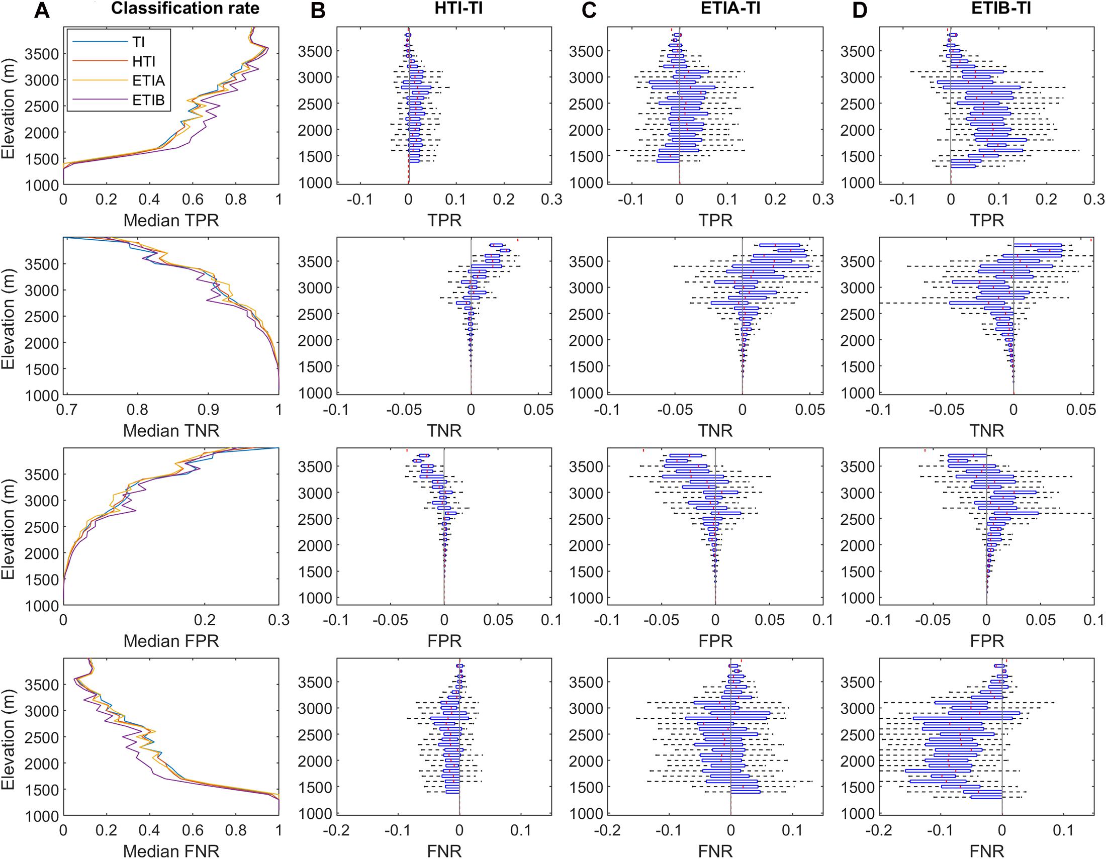
Figure 8. SCA classification errors by elevation; 1st row, true positive rate (TPR); 2nd row, true negative rate (TNR); 3rd row, false positive rate (FPR); 4th row, false negative rate. (A) Median error rate. (B–D) Differences between radiative and classical TI model.

Despite the overall good performance for the simple TI model, the enhanced models, especially ETIB, still explained more variability in SCA within most elevation bands, but with notable discrepancies among models (Figure 7). To better understand these discrepancies, the simulated SWE and melt rates were compared by elevation band (Figure 9). The HTI model shows the smallest difference relative to TI, in line with its more similar performance in SCA simulations. This can be attributed to the fact that HTI only adjusts the degree-day factor based on the potential clear-sky radiation and thus ignores temporal variations in atmospheric transmissivity and albedo. On the other hand, both ETI models show significant differences in simulated SWE (Figures 9C,D) and melt rates (Figures 9G,H) relative to TI. The best performing ETIB model simulates smaller melt rates and larger SWE at middle elevations (2000–3500 m), and higher melt rates and smaller SWE at the highest elevations (>3500 m). Interestingly, the median differences in SWE and melt rates between the enhanced models and TI per elevation band are rather small, which again shows that the preponderant influence of elevation on the simulated SWE is well captured by the simple TI model. However, significant deviations occur, up to ca. ± 20 mm for SWE and ca. ± 1 mm d^–1 for melt rates (Figures 9C,D,G,H). Given that the simulated SWE diverges most between models from March onto the melt season (Figure 5), it is intriguing that these significant differences in melt rates and SWE do not result in larger inter-model differences in simulated SCA and more so between the simulated SCA and MODIS SCA (Figure 7). This suggests that these differences in the spatial heterogeneity of melt rates between models may not be adequately captured by the pixel resolution of MODIS snow cover maps, a topic explored in the next section.

FIGURE 9

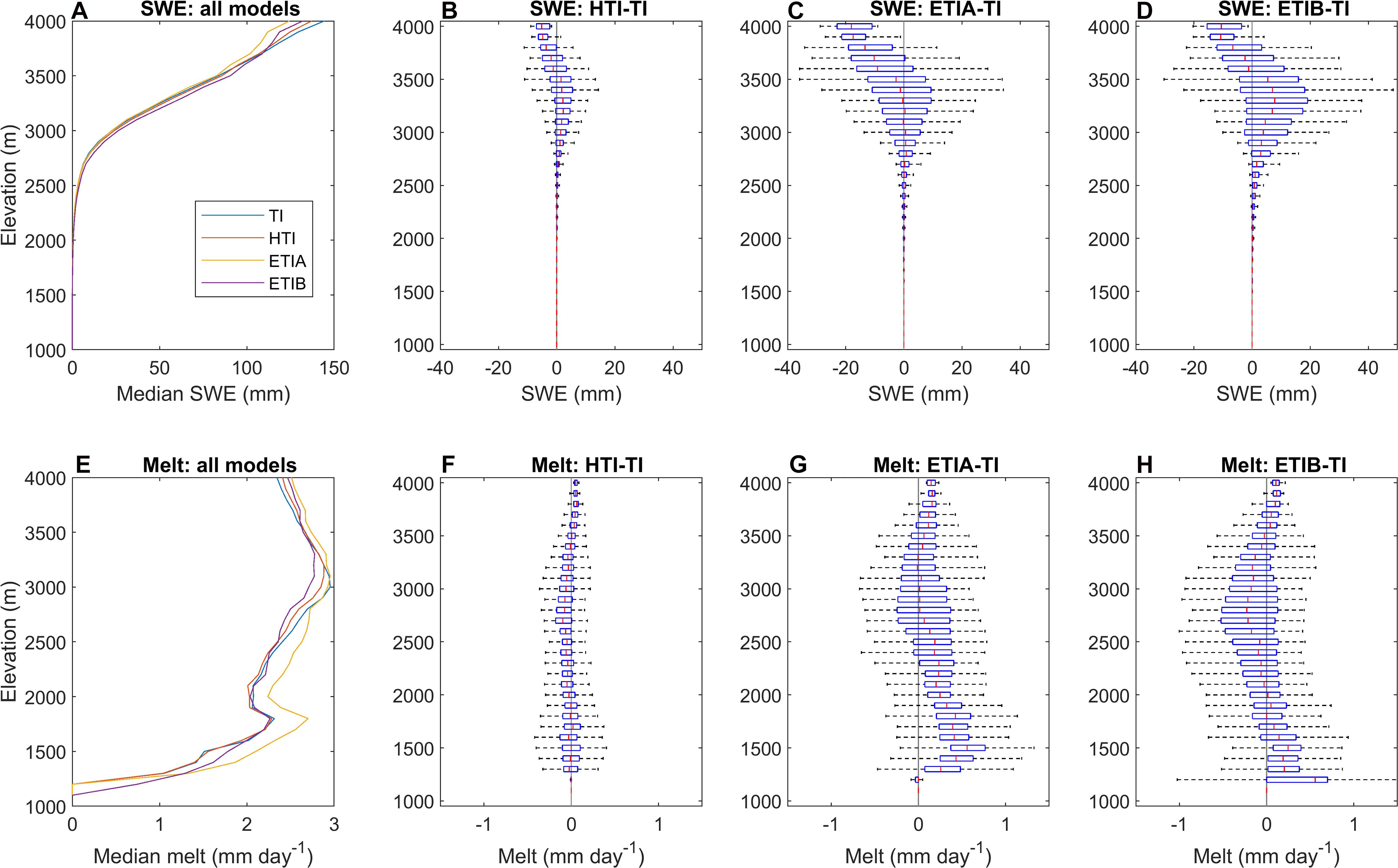
Figure 9. Mean simulated SWE and melt by elevation for days with snow. (A) Median SWE for all models. (B–D) SWE differences between radiative and reference TI model. (E) Median melt rate for all models. (F–H) Melt differences between radiative and TI model.

Effect of Spatial Resolution on SCA Validation

In order to compare the simulated SCA with MODIS, the modeled SCA was aggregated from 100 m to the 500 m resolution of MODIS (Figure 2). This has the potential to suppress significant spatial variability in the finer (100 m) scale simulated SCA. To explore this further, the mean snow cover duration (SCD = mean SCA × 365 days) simulated at the original 100 m resolution was compared to that aggregated at the MODIS 500 m resolution by aspect (Figure 10). The smoothing effect of model aggregation is particularly evident: at the original 100 m model resolution, all radiative models expectedly simulate smaller melt rates and larger SWE on northern slopes, and vice-versa on southern slopes (Figures 10A,B), which results in longer-lasting snow on northern slopes compared to the TI model (Figure 10C). Aggregation of the simulated SCA from 100 m to 500 m results in significant disruption of this pattern (Figure 10D), which can be attributed to changes in the distribution of slopes and aspects following aggregation (Figure 10E).

FIGURE 10

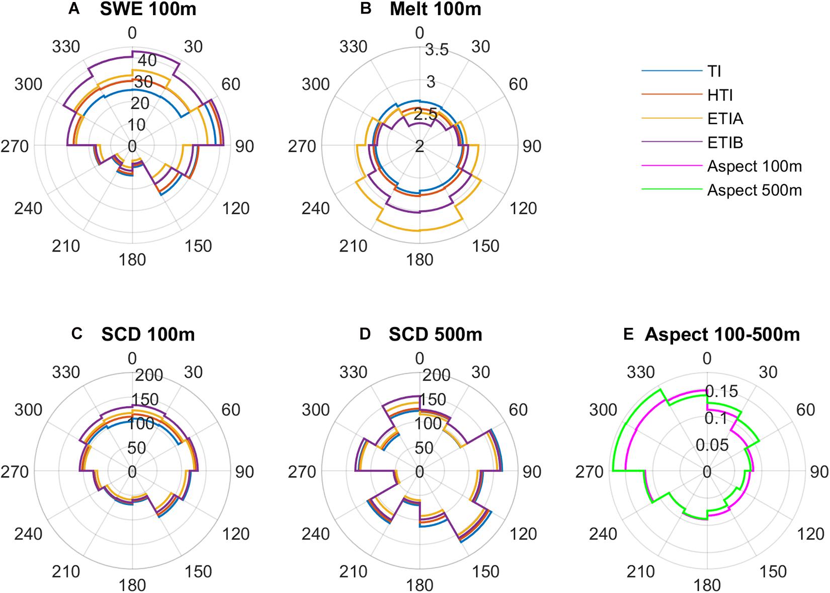
Figure 10. Mean simulated SWE, melt rate, and snow cover duration (SCD) by aspect. (A) Mean SWE (mm). (B) Melt rate (mm d^–1). (C) SCD (days) at 100 m resolution. (D) SCD (days) at 500 m resolution. (E) DEM aspect at 100 and 500 m resolution.

To better constrain the influence of scaling effects on the simulated SCD at 100 m resolution and its relationship with MODIS, the subgrid variability (standard deviation) was calculated for different pixel aggregation scales, from 200 m up to 1000 m (Figure 11A). Both ETI enhanced models clearly show higher subgrid variability than the TI model at scales below ~400 m, due to pronounced topographic-induced variability in solar radiation at those scales. The ETIB model, which includes albedo, shows the highest subgrid variability. The subgrid variability of MODIS (here resampled at 100 m) is expectedly low below its nominal resolution (500 m) and similar to that simulated by the TI and HTI models. At large aggregation scales (>400 m) elevation effects begin to dominate and the TI model displays more subgrid variability than the enhanced models, while the ETIB subgrid variability is most in line with MODIS. The influence of the aggregation scale on model intercomparison is seen in Figure 11B: the subgrid correlation between the enhanced models and the reference TI model decreases at scales below 700 m and show that the enhanced models are most different from TI below 400 m. However, the subgrid correlations between the simulated SCD and MODIS SCD show little differences between models, because MODIS does not sample the spatial variability below 500 m (Figure 11C). Hence, the consideration of global (ETIA) and net (ETIB) solar radiation introduces significant variability in SCD at scales not sampled by MODIS.

FIGURE 11

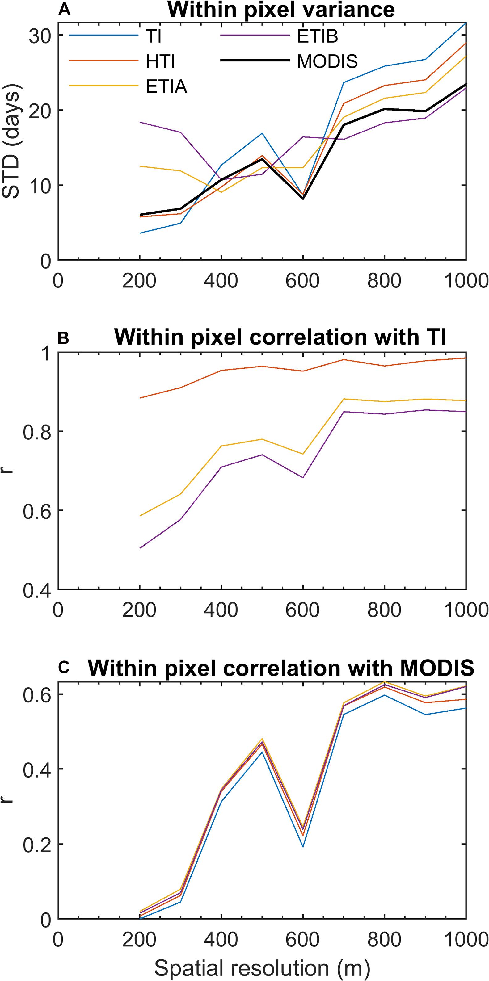
Figure 11. Scale analysis of snow cover duration (SCD, in days). (A) Subgrid (within pixel) variability (standard deviation) of simulated SCD at increasing aggregation scales. (B) Subgrid correlation between SCD simulated by the enhanced models and the reference TI model at increasing aggregation scales. (C) Subgrid correlation between SCD simulated by all models and MODIS SCD (resampled to 100 m resolution) at increasing aggregation scales.

Discussion and Conclusion

Difference in Model Performance

The enhanced radiative models, especially ETIB, showed increased performance relative to the simplest TI model for predicting basin wide SCA over time (Figure 4). In particular, the peak SCA in February was notably better simulated by the ETIB model compared to the other models (Figure 5C). However, overall differences in model performance were small. Our results show that most of the snow cover variability is driven by elevation and that this trend was adequately captured by all four models (Figure 7). Hence the simple TI model could be considered sufficient for melt simulations at the basin scale, due to the strong dependence of temperature and related melt rates on elevation, as found elsewhere (e.g., Vincent, 2002; Hock, 2003; Réveillet et al., 2017). While the enhanced radiative models improved the snow cover simulations as benchmarked by MODIS snow cover maps, their significant extra computational cost implies that the simpler TI would be adequate for operational snow simulations in this basin. This contrasts with previous studies that showed that including solar radiation improves the performance of spatially distributed melt models for predictions of glacier mass balance (Gabbi et al., 2014), snow cover area (Cazorzi and Dalla Fontana, 1996; Follum et al., 2015), and streamflow from snow-fed basins (Brubaker et al., 1996; Follum et al., 2019). On the other hand, the use of a fully distributed (grid-based) model improved the simulations of SCA relative to semi-distributed temperature index models previously applied in this basin (Boudhar et al., 2009).

The increasing false positive error rate (FPR) and decreasing false negative error rate (FNR) with elevation suggest that there may be a persistent elevation bias in the simulated SCA (Figure 8), which is partly alleviated by the radiative models, in particular ETIB. This suggests that increasing global radiation with altitude due to higher atmospheric transmissivity and the consideration of snow albedo result in steeper ablation profiles compared to temperature-only melt calculations with the TI model.

The effect of model parameters uncertainties must also be considered. The remaining elevation trends in the error rates in Figure 8 point to lingering problems with the distribution of precipitation in the basin. The use of a constant non-linear lapse rate for the spatial interpolation of precipitation to the basin is an obvious limitation, common to many snow and hydrological models. Calibrating the maximum difference elevation (△Z_max) to limit the vertical extrapolation of precipitation may have limited the errors associated with this approach, but significant uncertainties remain around the precipitation lapse rate and its limiting range (△Z_max). A sensitivity analysis to an uncertainty of ± 200 m on △Z_max showed that the inter-model differences in simulated SWE and SCA performance relative to MODIS remained similar to those found in Figures 7, 9 (Supplementary Figures 4, 5). Still, better spatially distributed precipitation fields would be needed in the future to improve snow simulations for hydrological model applications in this basin. Outputs from numerical weather models are increasingly used for this purpose, but are still problematic for precipitation (Bellaire et al., 2011; Réveillet et al., 2020). Scaling precipitation inputs by measured snow distributions is another promising approach but requires costly airborne surveys to acquire reliable snow depth maps (Vögeli et al., 2016). Progresses in mapping snow depth from high-resolution stereoscopic satellites images could, however, open new avenues on this front (Marti et al., 2016). Assimilation of snow cover maps within snow models can also help reducing precipitations biases (Margulis et al., 2016; Baba et al., 2018), but this increases computation costs which need to be minimized for operational hydrological applications.

The choice of melt model parameters (Table 3) could also affect the results. Bouamri et al. (2018) showed that enhanced snowmelt models can suffer from parameter equifinality, i.e., several combination of temperature and radiation parameters leading to a similar melt performance. Hence giving more weight to radiation in an enhanced model would increase the spatial heterogeneity of snowmelt rates and increase its difference with the simple TI model, and vice-versa. However, calibrating the models on a longer period tended to reduce the parameter equifinality (Bouamri et al., 2018).

Effect of Spatial Resolution on SCA Validation

Several previous studies found that snow on south-facing slopes receive more solar radiation, generally melts faster and lasts shorter than on north-facing slopes in the Northern Hemisphere (e.g., López-Moreno and Stähli, 2008; Tong et al., 2009; Comola et al., 2015; Baba et al., 2019). This topographic-induced melt variability due to unequal radiation loading on slopes is mainly lost upon aggregation to the coarser MODIS scale. This scaling effect corroborates previous conclusions made by Baba et al. (2019) concerning the influence of DEM resolution on the simulation of snow cover in the Rheraya basin. Using the physically based model SnowModel (Liston and Elder, 2006), they found a significant degradation of model performance when aggregating the model DEM to resolutions of 500 m and beyond, which disrupted the representation of slopes in the basin and affected solar radiation variability. It is also in line with recent finding by Zhang et al. (2021) who found significant scaling effects in MODIS NDSI products, which weakened the ability to estimate fractional and binary snow cover from MODIS NDSI data in the complex topography of the Tibetan Plateau. Steele et al. (2017) also found that the spatial resolution of MODIS NDSI products can obscure fine spatial patterning in snow cover and limit its use over areas of patchy, discontinuous snow.

Comola et al. (2015) also who showed that the effects of solar radiation patterns on the hydrologic response of snow-covered basins are scale dependent, i.e., significant at small scales with predominant aspects, and weak at larger scales where aspects become uncorrelated and orientation differences average out. These authors further found that a calibrated TI model on scales larger than the aspect correlation length are well transferable. Their conclusions find support in our results:

(i) The inclusion of radiation patterns in the large Rheraya catchment has a small influence overall on basin-wide simulated average SWE and SCA compared to the reference TI model.

(ii) The influence of solar radiation on simulated SWE and melt rates is greatly suppressed when aggregating model outputs to the 500 m MODIS resolution, which smooths out radiation effects and brings the radiative models closer to simulations made with a simple temperature-based (TI) model.

Hence our results support the notion that in large basins (i.e., larger than the correlation length of the terrain), topographic-induced variations in solar radiation tend to average out so that mean simulated melt rates, SWE, and SCA do not differ greatly from using temperature alone to predict snowmelt. A more uniform distribution of slope aspects in a basin, such as observed here for Rheraya (Figure 10E), will reinforce this phenomenon. In the context of operational flow forecasting in the High Atlas Range, simple temperature index models could thus provide sufficiently accurate snowmelt estimates. The impact of including solar radiation patterns in snowmelt calculation on streamflow simulations will, however, have to be investigated in a future study.

Our findings call for caution when using medium resolution satellite products such as MODIS to calibrate or validate spatially distributed snow models. The necessary aggregation of finer-scale model outputs to a resolution larger than key processes scales, such as that where interactions between topography and solar radiation are greatest, will suppress valid model information. The increasing availability of publicly available high-resolution snow cover maps imagery (Gascoin et al., 2019) should progressively reduce our dependence on MODIS snow cover products and help crash-testing high-resolution snow models in the future.

Data Availability Statement

The MODIS data used in this study is openly available in the National Snow and Ice Data Center (NSIDC) at (https://nsidc.org/), and the meteorological data are available at LMI-TREMA (https://www.lmi-trema.ma/) or upon demand with the authors.

Author Contributions

HB: data processing, analysis, interpretation, and writing. CK: conceptualization, supervision, analysis, interpretation, and writing. AB: conceptualization, supervision, and interpretation. SG: interpretation and writing. LH: discussion and editing. AC: discussion and editing. All authors contributed to the article and approved the submitted version.

Conflict of Interest

The authors declare that the research was conducted in the absence of any commercial or financial relationships that could be construed as a potential conflict of interest.

Funding

This research was funded by the Natural Sciences and Engineering Council of Canada, grant number RGPIN-2015-03844 and the Canada Research Chair program, grant number 231380 to CK, as well as by a Ph.D. scholarship from the CNRST (Centre National pour la Recherche Scientifique et Technique of Morocco) to HB. AC, AB, and LH are supported by the research program “MorSnow-1”, International Water Research Institute (IWRI), Mohammed VI Polytechnic University (UM6P), Morocco (Accord spécifique n° 39 entre OCP S.A et UM6P).

Acknowledgments

The authors would like to thank the Joint International Laboratory TREMA (http://trema.ucam.ac.ma) for providing meteorological data in the Rheraya basin.

Supplementary Material

The Supplementary Material for this article can be found online at: https://www.frontiersin.org/articles/10.3389/feart.2021.640250/full#supplementary-material

References

Abudu, S., Cui, C.-L., Saydi, M., and King, J. P. (2012). Application of snowmelt runoff model (SRM) in mountainous watersheds: a review. Water Sci. Eng. 5, 123–136.

Google Scholar

Aguilar, C., Herrero, J., and Polo, M. J. (2010). Topographic effects on solar radiation distribution in mountainous watersheds and their influence on reference evapotranspiration estimates at watershed scale. Hydrol. Earth Syst. Sci. 14, 2479–2494. doi: 10.5194/hess-14-2479-2010