The Impact of Applying Individually Perturbed Parametrization Tendency Scheme on the Simulated El Niño-Southern Oscillation in the Community Earth System Model

The ensemble technique is considered to be an effective approach in enhancing the model capacity of intra-seasonal climate change. Since El Niño-Southern Oscillation is one of the critical modes of interannual variability in the tropical Pacific, an appropriate ensemble technique may help minimize model bias in ENSO forecast. This research includes a modified stochastically perturbed parameterization tendencies scheme in the Community Earth System Model to investigate its impact on ENSO prediction. This revised scheme uses independent noise patterns to perturb the tendencies from different physical parameterizations. In the original scheme, only the same noise is employed. The result suggests that the altered approach is in a position to further reduce sea surface temperatures and gain more skill in uncertainty estimation compared to the original one. ENSO’s amplitude is improved especially of its warm phase El Niño, but there is a limited improvement in its spatial structure. The modified scheme also ameliorated the variability of ENSO by increasing the magnitude toward observation. The power spectrum exhibits an increased representation. Besides those findings, we notice that simple ensemble mean may not be able to represent the climate status as it smoothes out some useful signals.

Introduction

El Niño-Southern Oscillation (ENSO) is one primary mode of tropical variability phenomenon in the climate system (Rasmusson and Carpenter, 1982). Its warm phase (El Niño) is associated with the central and eastern equatorial regions with sea surface temperatures (SSTs) above normal. Opposite-signed changes occurred during the cold period (La Niña) (Deser et al., 2017). This naturally occurring fluctuation originates in the tropical Pacific zone. It affects the weather across the globe, including the impact on precipitation strength in the monsoon season and hurricane numbers affecting America (Ropelewski and Halpert, 1996; Bove et al., 1998). Because of ENSO’s crucial role in controlling climate, it has been the focus of intense investigation in recent years (Wang and Fiedler, 2006).

Effective ENSO forecasts could provide a chance for policy planners to take into consideration estimated climate abnormalities that could minimize the economic and cultural damage suffered by this climate event. A variety of studies have shown that coupled atmospheric-ocean general circulation models (CGCMs) have been an important tool for ENSO prediction (Paolino et al., 2012; Levine and Jin, 2015; Wu et al., 2015; Zhang et al., 2015; Kumar et al., 2016; Barnston et al., 2019; Wang et al., 2020). Despite the fact that the model improves during the last few decades, there remain systemic errors and other shortcomings in ENSO simulation even with state-of-the-art climate models (Bauer et al., 2015; Kumar et al., 2016; Vega-Westhoff and Sriver, 2017; Haszpra et al., 2020; Watterson et al., 2020). Despite using the data assimilation technique to initialize the model, fully coupled models still have deficiencies and are marginally better than the mathematical models in the ENSO process and intensity prediction. ENSO’s predictability is still constrained by various errors such as model, initial condition, and stochastic “noise” of the atmosphere (Moore and Kleeman, 1999; Balmaseda and Anderson, 2009). Numerous attempts, such as statistics, statistical dynamics, and ensemble techniques, are widely applied to ENSO predictions to increase predictability (Lau and Nath, 2006; Wang and Fiedler, 2006; Neale et al., 2008; Kirtman and Min, 2009; Zhang et al., 2013; Brown et al., 2015; Levine and Jin, 2015; Wu et al., 2015; Zhang et al., 2015; Atwood et al., 2016; Kumar et al., 2016; Levine et al., 2016; Vega-Westhoff and Sriver, 2017; Maher et al., 2018; Wang et al., 2020). Subsequent studies have suggested that model errors, especially uncertainty that raised from parametrization, generally have more impact than initial conditions, especially in climate prediction models (Stainforth et al., 2005; Christensen et al., 2015a; Christensen et al., 2017a; Yang et al., 2019). Thus, using ensemble approaches to estimate model errors and increase forecasting skills is recommended by the scientific community (Berner et al., 2016).

The European Centre for Medium-Range Weather Forecasts (ECMWF) has employed the stochastic parameterization scheme describing unresolved subgrid (Berner et al., 2009; Palmer et al., 2009; Leutbecher et al., 2017). This new ensemble approach is capable of sampling the instability of unsolved atmospheric processes, and this technique could be modified to monitor the model error representation capability. Including this zero-mean noise term in the general circulation model (GCM) can reduce model biases, increase ensemble spread, and forecast skill. Even in the absence of nonlinearity, this multiplicate noise is still able to shift the mean climate of the model, which is beneficial to model performance (Lin and Neelin, 2000, 2003; Berner et al., 2009; Christensen et al., 2015b; Berner et al., 2015; Berner et al., 2016).

Multiple studies have elucidated the significance of stochastic processes in ENSO forcing (Flügel et al., 2004; Yeh and Kirtman, 2006). The value of stochastic perturbation is recognized in ocean modeling already (Hasselmann, 1976). However, this stochastic approach has not been widely investigated in coupled climate models (Yang et al., 2019). Christensen et al. (2017b) applied the stochastically perturbed parametrization tendency (SPPT) scheme into the Community Climate System Model version 4 (CCSM4) and found that this scheme can reduce excessive ENSO spectrum power. The overestimated ENSO magnitude was also reduced due to improved zonal wind variability. Yang et al. (2019) followed Christensen et al. (2017b) and put both SPPT and stochastic kinetic energy backscatter (SKEB) schemes into the European Community Earth-System Model (EC-Earth), resulting in the improvement of the excessively weak representation of ENSO.

Wu et al. (2019) adjusted SPPT and applied this stochastic scheme to estimate the uncertainty introduced by cumulus parameterization in the Weather Research and Forecasting (WRF) model, finding that this modified approach could substantially reduce precipitation bias. Christensen et al. (2017b) and Wastl et al. (2019) proposed that different parametrization schemes or tendencies terms may have distinctive errors. Those schemes or terms should be perturbed with independent noise patterns. The independent SPPT (iSPPT) can accomplish this idea and results in an increase in model spread as well as model performance.

According to Neale et al. (2008), altering the deep convection parameterization will adjust the performance of ENSO representation in CCSM3. This may ring a bell that each parametrization may play a different role when attempting to simulate ENSO, and various parametrization processes, even in separate tendency terms, may yield different error characteristics. However, Christensen et al. (2017b) and Yang et al. (2019) did not use iSPPT for ENSO prediction. We consider this independent perturbation, especially on convection parameterization, which may be beneficial on ENSO forecasting. According to Wastl et al. (2019), applying different perturbations on different tendency terms can further raise the model performance. We assume that this independent perturbation approach, on both separate parametrization processes and distinct tendency terms, is more reasonable to represent the model error. Therefore, this paper includes a modified version of SPPT scheme into the Community Earth System Model (CESM) and investigates its impact on ENSO prediction as well as model performance. In addition, modified SPPT grouped the tendency terms to make the numerical model more robust and stable.

Model, Methods, Experiments, and Data

CESM 1.2.2 and Configuration

The CESM is a fully coupled global climate model. It was developed and is maintained by the National Center for Atmospheric Research (NCAR). In this research, version 1.2.2 is employed to explore the impact of different stochastic physics. More precisely, the stochastic parameterization scheme is implemented into CAM version 4, the atmosphere component model of CESM. The primary reason to choose CESM is that previous studies have shown that CESM exhibits a certain degree of competence in simulating climate change and annual variability, as well as the inter-decade change in the East Asian climate (Li et al., 2016; Vega-Westhoff and Sriver, 2017; Jiang et al., 2020).

This fully coupled global climate model has several components. The atmosphere component is the Community Atmosphere Model (CAM). In this research, only CAM4 is activated. CAM4 uses a finite-volume dynamic core with a horizontal resolution of 0.9° × 1.25°. The focus of this paper is lower atmospheric and ocean status. Therefore, CAM4 is only running under 26 vertical levels of configuration. Ocean status is provided by the Parallel Ocean Program (POP). The component has approximately 1° horizontal resolution with 60 vertical levels. The sea-ice component usually shares the same resolution with the ocean. This research is no exception; the same 1° horizontal and 60 vertical levels are employed in the sea-ice model Community Ice CodE (CICE) and Community Ice Sheet Model (Glimmer-CISM). CESM also includes the Community Land Model (CLM) and the River Transport Model (RTM), which share the same resolution configuration as the atmosphere component.

The Stochastically Perturbed Parameterization Schemes

The Original SPPT Scheme

The original SPPT scheme is used wildly in the medium-range weather forecast. The European Centre is the first major operational model center to use this approach. Researchers test this method in much smaller scales, such as convective allowing scale (Dorrestijn et al., 2013). Various climate models apply this very scheme to archive better results (Berner et al., 2016; Christensen et al., 2017a). The original SPPT scheme is also referred to as the Buizza–Miller–Palmer (BMP) scheme (Buizza et al., 1999). The BMP scheme was later replaced by a more efficient spectral pattern generator created by Palmer et al. (2009). This SPPT scheme assumes that the method of averaging is not effective and that parameterization uncertainties are representable as multiplicative noise terms. The noise used in the SPPT scheme is a random two-dimensional field, with temporal and spatial correlations; the amputation of each perturbation is limited to within [−2σ, 2σ], where σ denotes one standard deviation; this standard deviation is prescribed before generating perturbation pattern. The perturbed net tendency term (x) at each gridpoint is shown in formula (1):

$x=x_{\text{dyn}}+x_{\text{diffusion}}+\left(1-r\right)\cdot x_{\text{param}},(1)$

where $x_{\text{dyn}}$ represents tendency calculated from model dynamical processes, $x_{\text{diffusion}}$ stands for horizontal diffusion term, and $x_{\text{param}}$ represents the tendencies from parametrization processes. More precisely, $x_{\text{param}}$ denotes various parametrization physics tendencies combined. The SPPT scheme intends to represent the effects of subgrid-scale fluctuations. Therefore, the model’s dynamic tendency is not necessary to touch. Zhijie et al. (2011) also showed that a perturbation on dynamic tendency will not yield the desired outcome.

The detailed information about how to generate a random field $r$ is described in Berner et al. (2015). Nevertheless, what is different in this research is that we limit $r$ in the range of [−1,1] to avoid reverting the sign of tendency term, which also helps to avoid numerical instability. According to Christensen et al. (2017a), the suitable parameters for the global coupled climate model are horizontal decorrelation 500 km and temporal decorrelation of 6 h. The same setting is also applied in this research for inter-comparison purposes.

Most studies suggest that the near-surface perturbation may be too strong due to relatively large tendencies in the stratosphere (Bouttier et al., 2012; Berner et al., 2015; Jankov et al., 2019; Lock et al., 2019; Wastl et al., 2019). Therefore, we slightly deviated from Christensen et al. (2017a) and smoothly reduced the perturbation to zero at the surface and in the stratosphere for more stable model runs.

The Modified SPPT Scheme

As stated above, Christensen et al. (2017b) suggest that different parameterizations should be independently perturbed due to different error characteristics or properties. Wastl et al. (2019) also recommended such a strategy, but took one step further, using a different pattern to perturb various tendency terms. Interestingly, this approach is the original BMP scheme, which is the prototype of the SPPT scheme, we are trying to use, but quickly dropped due to instability reasons. There is no sufficient research for a decisive conclusion on whether the tendency terms should be perturbed independently or not. But for different parameterizations, this independent perturbation should be applied.

According to those researches, we modified the original SPPT scheme used in Christensen et al. (2017b) and let the altered scheme have the following ability: 1) each parametrization process, especially deep convection, can be perturbed independently; 2) tendency terms can be perturbed by two groups, wind tendency terms (U and V) and temperature and moist tendency terms (T and Q). This is unlike the Wastl et al. (2019) approach, four tendency terms (U, V, T, and Q) are perturbed by four independent noise pattern. The purpose of deviating from Wastl et al. (2019) is that we observe numerical instabilities during integration while using all different patterns on those four tendency terms.

In order to compare with the original scheme, we used the same parameters to generate perturbation in this modified scheme, which is horizontal decorrelation 500 km and temporal decorrelation of 6 h. The gridpoint variance is set to 0.5 because this is an empirical value.

Figure 1 shows the perturbation pattern snapshots in two continuous timesteps.

FIGURE 1

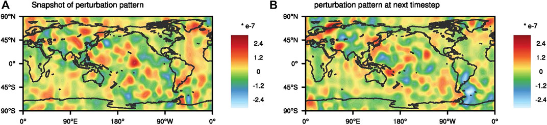
FIGURE 1. Snapshots of perturbation pattern used in this research. These two snapshots are taken from two continuous timesteps of the model.

Experiments Setup

To show the efficacy of the altered SPPT scheme and compare it to the original scheme, three sets of experiments are performed. These three sets are control (CTRL) experiments without stochastic physics, SPPT experiments employing the original stochastic scheme, and modified SPPT (ModSPPT) experiments.

Control Experiment

The control experiment aims to demonstrate the original performance of the coupled climate model and evaluate how accurate the ensemble system is when simulating the recent past. The historical integrations cover the period of 1850–2000, with the forcing from the fifth Coupled Model Intercomparison Project (Taylor et al., 2012). The period from 1850 to 1870 is used as a spin-up run in order to have a more favorable ocean state to run with the atmosphere model. The control experiment includes four members. The first member uses standard forcing without any ensemble technique. Member 2 is applying the same forcing but started with two days of the lagged ocean state. The configurations of members 3 and 4 are the same as those of member 2, but the ocean state is lagged for three and four days, respectively. Figure 2 demonstrates the experiment setup and configuration. This control experiment is labeled as CTRL.

The Experiment Using the Original SPPT Scheme

The SPPT experiment also involves four members, and those members share the same settings as CTRL. But in this experiment, the four total tendency terms (U, V, T, Q, as described in “The Original SPPT Scheme” section in the CAM4 model) are perturbed using the same noise pattern created by the spectral pattern generator. “The Original SPPT Scheme” section includes the specifics about the design of this scheme. The experiment using the original SPPT method is marked as SPPT.

The Experiment Using the Modified SPPT Scheme

As discussed above, different parameterizations should be perturbed separately since they have different error profiles. Therefore, in this experiment, radiation, convection, boundary layer processes, and other parameterizations are perturbed using different noise patterns. Wind tendency terms (U and V) in the same parameterization are perturbed by one noise pattern, and temperature and moist tendency terms (T and Q) in the same physics are perturbed by another noise pattern. The experiment using the original SPPT method is marked as ModSPPT.

Observations and Reanalysis Data

The observations and reanalysis data of sea surface temperature (SST) used in this paper for comparison are the Hadley Centre Global Sea Ice and Sea Surface Temperature (HadISST) version 1 (Rayner et al., 2003).

This paper makes use of the Climate Variability Diagnostics Package (CVDP) of the Community Earth System Model working group (Phillips et al., 2014) to compute various indices. Some figures in this manuscript were also using code from this package.

Results

Ensemble Performance

Since this study focuses on the ensemble method employed in a coupled climate model, the first question we want to address is how different ensemble approaches behave. Moreover, SST offers critical information on the global climate system, notably useful for detecting the El Niño and La Niña periods. Therefore, we concentrate on the model simulation capacity of SST. The root-mean-square error (RMSE) and ensemble spread were used as evaluation criteria.

Figure 3 displays global SST RMSE between model runs and HadISST. The RMSE is calculated for all four ensemble members; then averaged RMSE is displayed in this plot. Error bars show the standard deviation across different ensemble members. This plot suggests that both different stochastic physics schemes can reduce SST RMSE at least 15%, and modified SPPT can further reduce SST bias. The CTRL experiment has a relatively large bias in January, February, and March, which will result in a significant impact on ENSO forecast and simulation. But applying SPPT and ModSPPT scheme, this RMSE is decreased by 0.384 and 0.39 in January, 0.465 and 0.468 in February, and 0.462 and 0.469 in March. These RMSE reductions, despite small but nonzero differences in SPPT and ModSPPT scheme, imply that perturbing parameterization physics and tendencies with independent noise patterns will increase the performance of the ensemble system, at least in SST simulation.

FIGURE 2

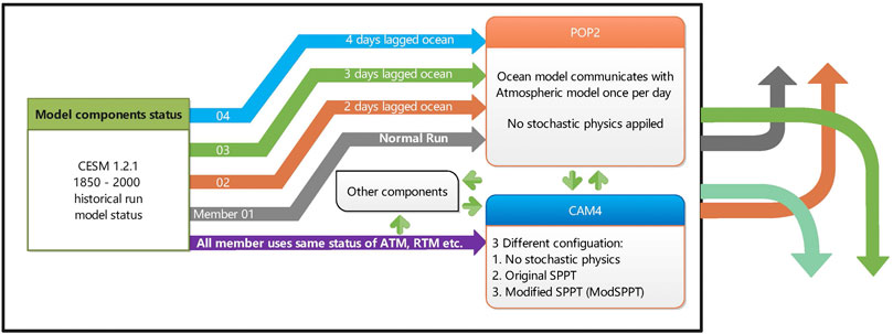
FIGURE 2. The diagram of the ensemble experiment setup.

FIGURE 3

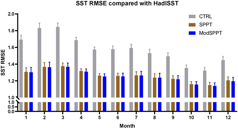
FIGURE 3. Ensemble mean RMSE of global SST in different months. The RMSE is calculated between the observations and model simulations.

Ensemble simulations usually allow measuring uncertainty among the systems by calculating the variance of ensemble members to quantify the spread within the ensemble. Although increased ensemble spread does not necessarily mean the best result, this score is an important criterion to identify the performance of the ensemble system. Another diagnostic that is often used to evaluate the ensemble system is the comparison of the standard deviation to the RMSE of the ensemble mean (RMSE/STD) ratio. Figure 4 displays both the spread and RMSE/STD to identify the skill of different ensemble approaches. The ModSPPT has a relatively large spread at practically all months, except February, March, and April, which have almost the same spread as the original SPPT scheme. SPPT, on the other hand, also increases model spread but not as much as ModSPPT does. This suggests that ModSPPT has more capability to estimate model uncertainty. RMSE/STD provides a more reasonable comparison of these two approaches. This ratio led to the same conclusion that ModSPPT has better performance in coupled climate ensemble system. The CTRL experiment fails behind SPPT and ModSPPT due to large RMSE in SST simulation.

FIGURE 4

FIGURE 4. The spread of different sets of experiments and RMSE/spread ratio. Dotted lines indicate the spread of each experiment; solid lines show the ratio of RMSE dividing by ensemble spread. Blue, brown, and gray exhibit the result of ModSPPT, SPPT, and CTRL, respectively.

Those multiple comparisons prove that the assumptions we proposed are beneficial for the coupled climate ensemble system. We also observe model outputs 6–9 “QNEG” or “QNEG” violation warnings every timestep during SPPT runs but only 3–5 warnings in CTRL and ModSPPT runs. Although this is within the normal range, this may suggest that ModSPPT perturbation is more favorable for CESM 1.2.2, and SPPT may need more turning. Despite this, stochastic physics can still increase model performance, especially the ModSPPT scheme, perturbing parameterization physics and variables with independent noise.

Impact on ENSO Simulation

The ENSO Spatial Composite

Many researchers suggest that most models have deficiencies that will cause systematic errors in both amplitude and temporal variability when simulating ENSO events (Lau and Nath, 2006; Kirtman and Min, 2009; Wu et al., 2015; Kumar et al., 2016; Wang et al., 2020; Watterson et al., 2020). Although the coupled climate model has improved over time, those deficiencies could be equally present in the CESM 1.2.2 model. The composite of El Niño and La Niña events is usually used to evaluate model performance. In this research, the definition of ENSO is based on a time series of SST in the box of 170°W–120°W, 5°S–5°N. Seasonal average SST in boreal winter (DJF; December, January, and February) is used to classify if a year is El Niño or La Niña. If the SST average exceeds one standard deviation of the monthly mean in the corresponding experiment output, it is called El Niño this year. Below one standard deviation will be considered as La Niña. Typically, only the ensemble mean is used for classification and evaluation. Since the first member of the CTRL experiment has the same configuration as the 1850–2000 historical run, it can therefore be treated as a reference to the deterministic forecast, so we also include the first member of three different sets of experiments for assessment purpose. Besides that, there is also a study on the original SPPT results of the CCSM 4 model with just one member (Christensen et al., 2017a).

Figures 5 and 6 show spatial composites of El Niño and La Niña in different ensemble approaches. The results are produced from the averaging model outputs obtained from all the years that have been defined as El Niño or La Niña by Niño-3.4 time series. The colors indicate the average SST anomaly for corresponding events. Over the land, SST anomaly is replaced with surface air temperature anomaly.

FIGURE 5

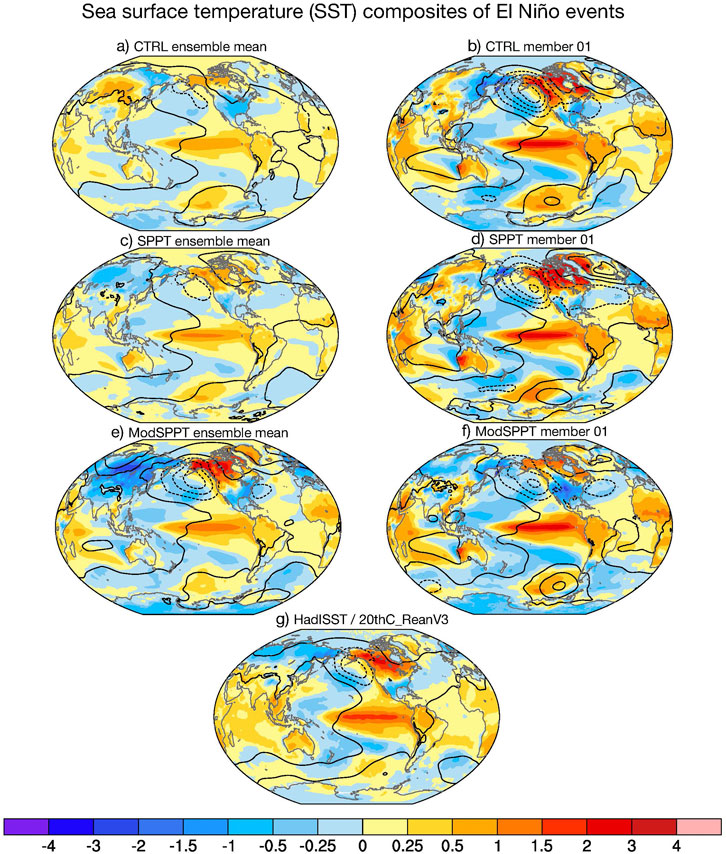
FIGURE 5. The spatial composite of El Niño for (A) ensemble mean CTRL, (B) first member of CTRL, (C) ensemble mean SPPT, (D) first member of SPPT, (E) ensemble mean ModSPPT, (F) first member of ModSPPT, and (G) observations. The shaded area repersent the sea air temperature anomaly over the ocean, and surface air temperature anomaly over land.

FIGURE 6

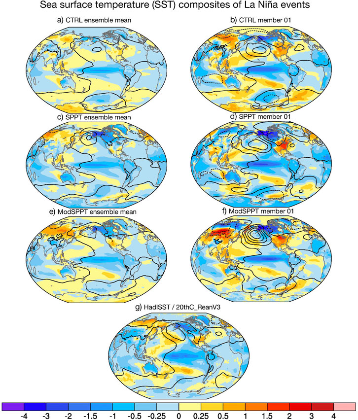
FIGURE 6. Same as Figure 5 but of La Niña.

The spatial structure of El Niño anomaly is well simulated by the CTRL experiment, as displayed in Figure 5, as well as two different stochastic physics schemes. The width and extent of warm tongue suggested by HadISST are reasonably simulated in all three sets of experiments, including both ensemble mean and the first member of experiments. However, the CTRL run shows a much weaker anomaly in the ensemble mean, whereas the original SPPT scheme can correct this by increasing the amplitude of El Niño. This result is consistent with that of Yang et al. (2019), who used SPPT combined with another stochastic physics. Even though ModSPPT is able to further increase the skill of the model, in particular, the Central Eastern Pacific Ocean with the highest magnitude of El Niño is comparable to that of HadISST. But, model results for the first member of the ensemble are quite different from the ensemble average. Member 1 of the CTRL experiment has a stronger magnitude of El Niño than observation. This indicates that CESM 1850–2000 historical run has a warm bias of El Niño simulation and is consistent with previous studies (Kirtman and Min, 2009; Berner et al., 2016; Christensen et al., 2017a). Employing only stochastic physics in the deterministic forecast, as Christensen et al. (2017a) did in their research, can also increase the model skill by reducing this bias in El Niño simulation. ModSPPT, on the other hand, is even more effective in bringing model simulation close to HadISST. This modified SPPT scheme yielded the best results in this comparison.

La Niña anomaly is also captured by these three sets of experiments but not as well as El Niño. Figure 6 suggests that, in La Niña events, this anomaly structure is not extending far enough as HadISST does. These three experiments face the same dilemma. For the magnitude, the ensemble mean of CTRL experiment has not enough cold anomaly at the equator, whereas SPPT can increase this anomaly by about 0.5°. ModSPPT cannot improve La Niña anomalies compared to SPPT; however, this modified scheme is still yielding a better result than CTRL. This comparison finding also holds for the first member of different experiments, except that the bias is in another direction (too cold).

We use two different scores to quantify the performance of the model. The pattern correlation (PC) generally shows how the model simulates the ENSO structure, and root-mean-square (RMS) differences show how far the model deviates from observations, with that score being displayed in Figure 7. In this plot, the red color indicates a better result. The TAS is used here instead of SST because we also want to include temperature over land. The PC of ENSO TAS in DJF is displayed. We found that stochastic physics can increase the forecast skill of ENSO spatial structure. However, PC shows no significant difference between SPPT and ModSPPT, indicating that ModSPPT is unable to gain benefit while the model trying to simulate ENSO structure. However, the RMS difference has been reduced from 0.53 to 0.49, implying that the forecast skill of ENSO magnitude has been increased when modifying the original SPPT scheme.

FIGURE 7

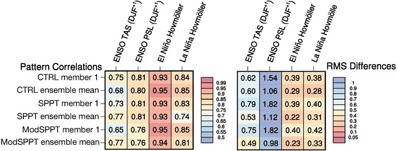
FIGURE 7. Pattern correlation scores and RMSD scores. Red indicates the desired result, which shows better performance. Blue suggests the opposite conclusion.

Figure 8 is the El Niño and La Niña composite Hovmöller diagrams of HadISST and ensemble mean status of different sets of experiments. This plot suggests that numeral simulation can capture the main pattern of El Niño and La Niña, as shown in Figures 5 and 6. SPPT has closer amplitude to observation, whereas ModSPPT corrects the pattern. The quantified result proves the La Niña Hovmöller pattern, and the SPPT scheme is not well simulated in previous research (Christensen et al., 2017a; Yang et al., 2019) improved by 0.07 in PC score. SPPT scheme can improve the performance in El Niño Hovmöller pattern, but ModSPPT is still able to gain that increment by 0.01 more.

FIGURE 8

FIGURE 8. Hovmöller diagrams of El Niño composites (A)–(D) and La Niña composites (E)–(H) for HadISST, ensemble mean CTRL, ensemble mean SPPT, and ensemble mean SPPT. SSTs are averaged between 5°S and 5°N.

The result of the El Niño and La Niña composites indicates that the application of stochastic physics to a coupled climate model is capable of improving the amplitude of ENSO in ensemble simulation, but less improvement in spatial structure. By changing the original SPPT scheme, ModSPPT could enable further enhancement of ENSO prediction. Applying those schemes in deterministic simulation, not a recommended approach but a practical one, still yields a favorable result when it comes to ENSO amplitude prediction.

The Temporal Variability of ENSO

Since fully coupled climate model simulation is used extensively in the ENSO variability investigation, in particular on decadal and longer time frames, therefore, whether ModSPPT is able to gain the skill of simulating ENSO in temporal variability is another question we want to answer.

The variability of ENSO can be diagnosed using the time series of Niño-3.4 annual cycle. Figure 9 shows ENSO by calculating the standard deviation of the monthly means in different experiments as well as HadISST. This is different from Figure 4, which is the ensemble mean of monthly means. Another difference is that Figure 9 only includes Niño-3.4, but Figure 4 demonstrates the global performance of ensemble approaches. From this plot, we can quickly diagnose that ModSPPT has the strongest variability compared to other ensemble methods in almost all 12 months. The increment of this benefit is more than 0.075, which is almost 15% of the CTRL ensemble mean. But all three sets of experiments show variability levels below HadISST, indicating that all ensemble systems underestimate the ENSO variability.

FIGURE 9

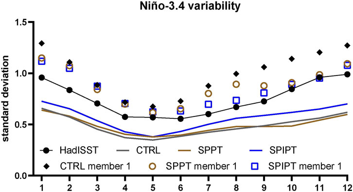
FIGURE 9. The monthly variability of Niño 3.4. Solid lines show the mean of the annual cycle in Niño-3.4 variability. This value is calculated by the standard deviation of the monthly means of the Niño-3.4 time series. Marks show the same value but for the first member only. Blue, brown, and gray show the result of ModSPPT, SPPT, and CTRL, respectively.

Various studies reporting applying ensemble mean without any weight may result in weaker ENSO variability (Atwood et al., 2016; Vega-Westhoff and Sriver, 2017). Only including one member will indeed get a stronger variability because the ensemble means usually smooth the result especially where the negative and positive change occurred in different members. Therefore, Figure 9 also included the first member of each set of experiments. This first member comparison suggests that ModSPPT is still able to bring the original SPPT scheme close to observation, whereas SPPT already weakens the overestimated variability in the CTRL experiment. The result from the first member, which has the same configuration as the deterministic historical run, proves that this modified SPPT scheme has better results as the ensemble means suggested.

The power spectrum is demonstrated in Figure 10. The CTRL has flattened and weaker response and missing 6–7 years oscillations. The 3–4 years oscillations are also significantly reduced. This is not similar to what previous researchers have found where CMIP5 coupled models may have narrow and sharp results. The deviation from previous researchers may also be due to the averaged ensemble result, which is smoothed too much. The SPPT scheme can preserve a 3-year signal but not as strong as HadISST. But ModSPPT is able to get a stronger signal on 2–3 years’ oscillations while having a 5-year signal. The effect of stochastic physics on ENSO is consistent with what’s seen in the CCSM, where warmer SSTs are correlated with strong El Niño events with a sharp ENSO power spectrum. However, the root of the problem requires further analysis such as using the delayed oscillator model.

FIGURE 10

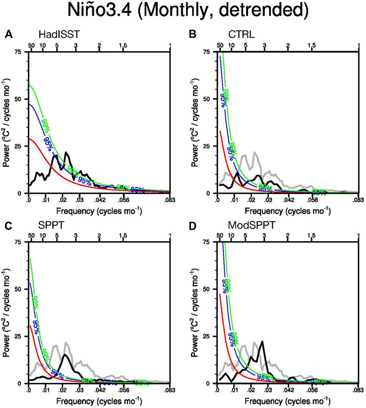
FIGURE 10. The power spectrum of the Niño 3.4 time series. The top x-axis suggests the period in years, and the bottom x-axis is the frequency in cycles per month. Blue and green lines are the 95 and 99% confidence bounds of the best-fit auto-regressive spectrum. This best-fit spectrum is shown as red lines.

The performance of the temporal variability of ENSO is boosted by introducing this modified SPPT scheme. It can increase underestimated Niño-3.4 variability and reduce the same variability when it comes to deterministic run. Results confirm that ModSPPT has better performance than the original scheme. We can also learn from this intercomparison that ensemble mean is not a satisfactory summary statistic since the average of members could be almost zero when there is more significant variance in fact.

Discussion

This study demonstrates the performance of a modified SPPT scheme on ENSO simulation and prediction using CESM 1.2.2. Three sets of four-member historical ensemble experiments, including time-lagged CTRL, original SPPT scheme, and ModSPPT scheme, are analyzed and compared with observation. The main findings of this work are summarized as follows.

1)Applying independent noise patterns to different parameterization physics and different tendency terms is beneficial to model performance. The modified scheme is able to reduce global SST RMSE by 20.5% and increase the model spread by 21.6% compared to the CTRL experiment, that is, 0.4 and 6.2% performance boosts, respectively, compared to the original scheme. This comparison suggests that independent perturbation approaches are advantageous to CESM, similar to those performed in the convective-allowing scale model. But unlike such a scale, if all tendency terms are perturbed with the independent pattern, it will cause numerical model instability in CESM. Therefore, grouping the tendency terms and then applying the different patterns to that group is a more reasonable approach.

2)The stochastic physics can improve ENSO’s amplitude, but this modified SPPT scheme can further improve the amplitude of ENSO. Although there is less improvement in spatial structure, the ModSPPT scheme has the ability to boost the pattern correlation score of La Niña Hovmöller by 0.07 compared to the original scheme. This is primarily due to the increase in the ocean’s mean status in the tropical Pacific, where the major model has deficiencies. The variability also demonstrates amplitude increment for interannual timescales compared to the original scheme.

3)Both the first member of the ensemble system and ensemble mean of the modified scheme can show improvement but in a different manner. Ensemble means generally show underestimating amplitude and not enough ENSO variability, while the first member usually overestimates them. A simple average without any weighting of ensemble member status will result in ignoring the useful signals. This may call for proper weights, as Sun et al. (2017) proposed, to be determined before summarizing such a collection of projections.

Data Availability Statement

The raw data supporting the conclusions of this article will be made available by the authors, without undue reservation.

Author Contributions

TW designed the experiment and the computational framework and analysed the data SZ verified the numerical results. TW wrote the manuscript with support from SZ. Both KZ and HM contributed to the final version of the manuscript.

Funding

This work was sponsored by the National Key Research and Development Program of China (2016YFA0600402), National Key Research and Development Program of China (2018YFC1507604) and the National Natural Science Foundation of China (41975124).

Conflict of Interest

The authors declare that the research was conducted in the absence of any commercial or financial relationships that could be construed as a potential conflict of interest.

References

Atwood, A. R., Battisti, D. S., Wittenberg, A. T., Roberts, W. H. G., and Vimont, D. J. (2016). Characterizing unforced multi-decadal variability of ENSO: a case study with the GFDL CM2.1 coupled GCM. Clim. Dynam. 49 (7–8), 2845–2862. doi:10.1007/s00382-016-3477-9

CrossRef Full Text | Google Scholar

Balmaseda, M., and Anderson, D. (2009). Impact of initialization strategies and observations on seasonal forecast skill. Geophys. Res. Lett. 36 (1), 133. doi:10.1029/2008gl035561

CrossRef Full Text | Google Scholar

Barnston, A. G., Tippett, M. K., Ranganathan, M., and L, ’ Heureux, M. L. (2019). Deterministic skill of ENSO predictions from the North American Multimodel ensemble. Clim. Dynam. 53 (12), 7215–7234. doi:10.1007/s00382-017-3603-3

CrossRef Full Text | Google Scholar

Bauer, P., Thorpe, A., and Brunet, G. (2015). The quiet revolution of numerical weather prediction. Nature. 525 (7567), 47–55. doi:10.1038/nature14956 |

PubMed Abstract | CrossRef Full Text | Google Scholar

Berner, J., Achatz, U., BattÉ, L., Bengtsson, L., De La CÁMara, A., Christensen, H. M., et al. (2016). Stochastic parameterization: towards a new view of weather and climate models. Bull. Am. Meteorol. Soc. 98, 565–588. doi:10.1175/bams-d-15-00268.1

CrossRef Full Text | Google Scholar

Berner, J., Fossell, K. R., Ha, S. Y., Hacker, J. P., and Snyder, C. (2015). Increasing the skill of probabilistic forecasts: understanding performance improvements from model-error representations. Mon. Weather Rev. 143 (4), 1295–1320. doi:10.1175/mwr-d-14-00091.1

CrossRef Full Text | Google Scholar

Berner, J., Shutts, G. J., Leutbecher, M., and Palmer, T. N. (2009). A spectral stochastic kinetic Energy backscatter scheme and its impact on flow-dependent predictability in the ECMWF ensemble prediction system. J. Atmos. Sci. 66 (3), 603–626. doi:10.1175/2008jas2677.1

CrossRef Full Text | Google Scholar

Bouttier, F., Vie, B., Nuissier, O., and Raynaud, L. (2012). Impact of stochastic physics in a convection-permitting ensemble. Mon. Weather Rev. 140 (11), 3706–3721. doi:10.1175/mwr-d-12-00031.1

CrossRef Full Text | Google Scholar

Bove, M. C., Elsner, J. B., Landsea, C. W., Niu, X., and O’Brien, J. J. (1998). Effect of El Niño on U.S. Landfalling hurricanes, revisited. Bull. Am. Meteorol. Soc. 79. 2477–2482. doi:10.1175/1520-0477(1998)079<2477

CrossRef Full Text | Google Scholar

Brown, J. R., Hope, P., Gergis, J., and Henley, B. J. (2015). ENSO teleconnections with Australian rainfall in coupled model simulations of the last millennium. Clim. Dynam. 47 (1–2), 79–93. doi:10.1007/s00382-015-2824-6

CrossRef Full Text | Google Scholar

Buizza, R., Miller, M., and Palmer, T. N. (1999). Stochastic representation of model uncertainties in the ECMWF ensemble prediction system. Q. J. R. Meteorol. Soc. 125 (560), 2887–2908. doi:10.1256/smsqj.56005

CrossRef Full Text | Google Scholar

Christensen, H. M., Berner, J., Coleman, D. R. B., and Palmer, T. N. (2017a). Stochastic parameterization and El Niño–Southern oscillation. J. Clim. 30 (1), 17–38. doi:10.1175/jcli-d-16-0122.1

CrossRef Full Text | Google Scholar

Christensen, H. M., Lock, S. J., Moroz, I. M., and Palmer, T. N. (2017b). Introducing independent patterns into the stochastically perturbed parametrization tendencies (SPPT) scheme. Q. J. R. Meteorol. Soc. 143 (706), 2168–2181. doi:10.1002/qj.3075

CrossRef Full Text | Google Scholar

Christensen, H. M., Moroz, I. M., and Palmer, T. N. (2015a). Simulating weather regimes: impact of stochastic and perturbed parameter schemes in a simple atmospheric model. Clim. Dynam. 44 (7–8), 2195–2214. doi:10.1007/s00382-014-2239-9

CrossRef Full Text | Google Scholar

Christensen, H. M., Moroz, I. M., and Palmer, T. N. (2015b). Stochastic and perturbed parameter representations of model uncertainty in convection parameterization*. J. Atmos. Sci. 72 (6), 2525–2544. doi:10.1175/jas-d-14-0250.1

CrossRef Full Text | Google Scholar

Deser, C., Simpson, I. R., McKinnon, K. A., and Phillips, A. S. (2017). The Northern Hemisphere extratropical atmospheric circulation response to ENSO: how well do we know it and how do we evaluate models accordingly?. J. Clim. 30 (13), 5059–5082. doi:10.1175/jcli-d-16-0844.1

CrossRef Full Text | Google Scholar

Dorrestijn, J., Crommelin, D. T., Siebesma, A. P., and Jonker, H. J. J. (2013). Stochastic parameterization of shallow cumulus convection estimated from high-resolution model data. Theor. Comput. Fluid Dynam. 27 (1–2), 133–148. doi:10.1007/s00162-012-0281-y

CrossRef Full Text | Google Scholar

Flügel, M., Chang, P., and Penland, C. (2004). The role of stochastic forcing in Modulating ENSO predictability. J. Clim. 17, 3125–3140. doi:10.1175/1520-0442(2004)017<3125:TROSFI>2.0

CrossRef Full Text | Google Scholar

Hasselmann, K. (1976). Stochastic climate models Part I. Theory Tellus. 28 (6), 473–485. doi:10.1111/j.2153-3490.1976.tb00696.x

CrossRef Full Text | Google Scholar

Haszpra, T., Herein, M., and Bódai, T. (2020). Investigating ENSO and its teleconnections under climate change in an ensemble view—a new perspective. Earth System Dynamics. 11 (1), 267–280. doi:10.5194/esd-11-267-2020

CrossRef Full Text | Google Scholar

Jankov, I., Beck, J., Wolff, J., Harrold, M., Olson, J. B., Smirnova, T., et al. (2019). Stochastically Perturbed Parameterizations in an HRRR-Based Ensemble. 147 (1), 153–173. doi:10.1175/mwr-d-18-0092.1

CrossRef Full Text

Jiang, D., Si, D., and Lang, X. (2020). Evaluation of East Asian summer climate prediction from the CESM large-ensemble initialized decadal prediction Project. Journal of Meteorological Research. 34 (2), 252–263. doi:10.1007/s13351-020-9151-5

CrossRef Full Text | Google Scholar

Kirtman, B. P., and Min, D. (2009). Multimodel ensemble ENSO prediction with CCSM and CFS. Mon. Weather Rev. 137 (9), 2908–2930. doi:10.1175/2009MWR2672.1

CrossRef Full Text | Google Scholar

Kumar, A., Hu, Z.-Z., Jha, B., and Peng, P. (2016). Estimating ENSO predictability based on multi-model hindcasts. Clim. Dynam. 48 (1–2), 39–51. doi:10.1007/s00382-016-3060-4

CrossRef Full Text | Google Scholar

Lau, N. C., and Nath, M. J. (2006). ENSO modulation of the interannual and intraseasonal variability of the East Asian monsoon - a model study. J. Clim. 19 (18), 4508–4530. doi:10.1175/jcli3878.1

CrossRef Full Text | Google Scholar

Leutbecher, M., Lock, S.-J., Ollinaho, P., Lang, S. T. K., Balsamo, G., Bechtold, P., et al. (2017). Stochastic representations of model uncertainties at ECMWF: state of the art and future vision. Q. J. R. Meteorol. Soc. 143 (707), 2315–2339. doi:10.1002/qj.3094

CrossRef Full Text | Google Scholar

Levine, A. F. Z., and Jin, F. F. (2015). A simple approach to quantifying the noise–ENSO interaction. Part I: deducing the state-dependency of the windstress forcing using monthly mean data. Clim. Dynam. 48 (1–2), 1–18. doi:10.1007/s00382-015-2748-1

CrossRef Full Text | Google Scholar

Levine, A. F. Z., Jin, F. F., and Stuecker, M. F. (2016). A simple approach to quantifying the noise–ENSO interaction. Part II: the role of coupling between the warm pool and equatorial zonal wind anomalies. Clim. Dynam. 48 (1–2), 19–37. doi:10.1007/s00382-016-3268-3

CrossRef Full Text | Google Scholar

Li, X., Tang, Y., Zhou, L., Chen, D., Yao, Z., and Islam, S. U. (2016). Assessment of Madden–Julian oscillation simulations with various configurations of CESM. Clim. Dynam. 47 (7), 2667–2690. doi:10.1007/s00382-016-2991-0

CrossRef Full Text | Google Scholar

Lin, J. W.-B., and Neelin, J. D. (2000). Influence of a stochastic moist convective parameterization on tropical climate variability. Geophys. Res. Lett. 27 (22), 3691–3694. doi:10.1029/2000gl011964

CrossRef Full Text | Google Scholar

Lin, J. W.-B., and Neelin, J. D. (2003). Toward stochastic deep convective parameterization in general circulation models. Geophys. Res. Lett. 30 (4). doi:10.1029/2002gl016203

CrossRef Full Text | Google Scholar

Lock, S. J., Lang, S. T. K., Leutbecher, M., Hogan, R. J., and Vitart, F. (2019). Treatment of model uncertainty from radiation by the Stochastically Perturbed Parametrization Tendencies (SPPT) scheme and associated revisions in the ECMWF ensembles. Q. J. R. Meteorol. Soc. 145 (S1), 75–89. doi:10.1002/qj.3570

CrossRef Full Text | Google Scholar

Maher, N., Matei, D., Milinski, S., and Marotzke, J. (2018). ENSO change in climate projections: forced response or internal variability?. Geophys. Res. Lett. 45 (20). doi:10.1029/2018gl079764

CrossRef Full Text | Google Scholar

Moore, A. M., and Kleeman, R. (1999). Stochastic forcing of ENSO by the intraseasonal oscillation. J. Clim. 12, 1199–1220. doi:10.1175/1520-0442(1999)012<1199:SFOEBT>2.0

CrossRef Full Text | Google Scholar

Neale, R. B., Richter, J. H., and Jochum, M. (2008). The impact of convection on ENSO: from a delayed oscillator to a series of events. J. Clim. 21 (22), 5904–5924. doi:10.1175/2008JCLI2244.1

CrossRef Full Text | Google Scholar

Palmer, T. N., Buizza, R., Doblas-Reyes, F., Jung, T., M.L., , Shutts, G. J., et al. (2009). Stochastic parametrization and model uncertainty. ECWMF Tech. 598 (1), 1–44. doi:10.1007/978-3-658-15639-8_4

CrossRef Full Text | Google Scholar

Paolino, D. A., Kinter, J. L., Kirtman, B. P., Min, D. H., and Straus, D. M. (2012). The impact of land surface and atmospheric initialization on seasonal forecasts with CCSM. J. Clim. 25 (3), 1007–1021. doi:10.1175/2011jcli3934.1

CrossRef Full Text | Google Scholar

Phillips, A. S., Deser, C., and Fasullo, J. (2014). Evaluating modes of variability in climate models. Eos Trans. Am. Geophys. Union. 95 (49), 453–455. doi:10.1002/2014eo490002

CrossRef Full Text | Google Scholar

Rasmusson, E. M., and Carpenter, T. H. (1982). Variations in tropical sea surface temperature and surface wind fields associated with the Southern oscillation/el Niño. Mon. Weather Rev. 110, 354–384. doi:10.1175/1520-0493(1982)110<0354:VITSST>2.0

CrossRef Full Text | Google Scholar

Rayner, N. A., Parker, D. E., Horton, E. B., Folland, C. K., Alexander, L. V., Rowell, D. P., et al. (2003). Global analyses of sea surface temperature, sea ice, and night marine air temperature since the late nineteenth century. J. Geophys. Res.: Atmosphere. 108 (D14), 111–191. doi:10.1029/2002jd002670

CrossRef Full Text | Google Scholar

Ropelewski, C. F., and Halpert, M. S. (1996). Quantifying Southern oscillation-precipitation relationships. J. Clim. 9, 1043–1059. doi:10.1175/1520-0442(1996)009<1043:QSOPR>2.0

CrossRef Full Text | Google Scholar

Stainforth, D. A., Aina, T., Christensen, C., Collins, M., Faull, N., Frame, D. J., et al. (2005). Uncertainty in predictions of the climate response to rising levels of greenhouse gases. Nature. 433 (7024), 403–406. doi:10.1038/nature03301

PubMed Abstract | CrossRef Full Text | Google Scholar

Sun, X., Yin, J., and Zhao, Y. (2017). Using the inverse of expected error variance to determine weights of individual ensemble members: application to temperature prediction. J. Meteorol. Res. 31 (3), 502–513. doi:10.1007/s13351-017-6047-0

CrossRef Full Text | Google Scholar

Taylor, K. E., Stouffer, R. J., and Meehl, G. A. (2012). An overview of CMIP5 and the experiment design. Bull. Am. Meteorol. Soc. 93 (4), 485–498. doi:10.1175/BAMS-D-11-00094.1

CrossRef Full Text | Google Scholar

Vega-Westhoff, B., and Sriver, R. L. (2017). Analysis of ENSO’s response to unforced variability and anthropogenic forcing using CESM. Sci. Rep. 7 (1), 124–137. doi:10.1038/s41598-017-18459-8 |

PubMed Abstract | CrossRef Full Text | Google Scholar

Wang, C., and Fiedler, P. C. (2006). ENSO variability and the eastern tropical Pacific: a review. Prog. Oceanogr. 69 (2–4), 239–266. doi:10.1016/j.pocean.2006.03.004

CrossRef Full Text | Google Scholar

Wang, L., Ren, H.-L., Zhu, J., and Huang, B. (2020). Improving prediction of two ENSO types using a multi-model ensemble based on stepwise pattern projection model. Clim. Dynam. 54 (7–8), 3229–3243. doi:10.1007/s00382-020-05160-2

CrossRef Full Text | Google Scholar

Wastl, C., Wang, Y., Atencia, A., and Wittmann, C. (2019). Independent perturbations for physics parametrization tendencies in a convection-permitting ensemble (pSPPT). Geosci. Model Dev. (GMD) 12 (1), 261–273. doi:10.5194/gmd-12-261-2019

CrossRef Full Text | Google Scholar

Watterson, I. G., Risbey, J. S., Moore, T. S., Matear, R. J., Kitsios, V., Sandery, P. A., et al. (2020). Enhanced ENSO prediction via augmentation of Multimodel ensembles with initial thermocline perturbations. J. Clim. 33 (6), 2281–2293. doi:10.1175/jcli-d-19-0444.1

CrossRef Full Text | Google Scholar

Wu, T., Min, J., and Wu, S. (2019). A comparison of the rainfall forecasting skills of the WRF ensemble forecasting system using SPCPT and other cumulus parameterization error representation schemes. Atmos. Res. 218, 160–175. doi:10.1016/j.atmosres.2018.11.016

CrossRef Full Text | Google Scholar

Wu, X., Han, G., Zhang, S., and Liu, Z. (2015). A study of the impact of parameter optimization on ENSO predictability with an intermediate coupled model. Clim. Dynam. 46 (3–4), 711–727. doi:10.1007/s00382-015-2608-z

CrossRef Full Text | Google Scholar

Yang, C., Christensen, H. M., Corti, S., von Hardenberg, J., and Davini, P. (2019). The impact of stochastic physics on the El Niño Southern Oscillation in the EC-Earth coupled model. Clim. Dynam. 53 (5–6), 2843–2859. doi:10.1007/s00382-019-04660-0

CrossRef Full Text | Google Scholar

Yeh, S.-W., and Kirtman, B. P. (2006). Origin of decadal El Niño–Southern Oscillation–like variability in a coupled general circulation model. J. Geophys. Res.: Oceans. 111 (C1), 133–139. doi:10.1029/2005JC002985

CrossRef Full Text | Google Scholar

Zhang, D., Blender, R., and Fraedrich, K. (2013). Volcanoes and ENSO in millennium simulations: global impacts and regional reconstructions in East Asia. Theor. Appl. Climatol. 111 (3–4), 437–454. doi:10.1007/s00704-012-0670-6

CrossRef Full Text | Google Scholar

Zhang, H., Dong, G., Moise, A., Colman, R., Hanson, L., and Ye, H. (2015). Uncertainty in CMIP5 model-projected changes in the onset/retreat of the Australian summer monsoon. Clim. Dynam. 46 (7), 2371–2389. doi:10.1007/s00382-015-2707-x

CrossRef Full Text | Google Scholar

Zhijie, R., Jing, C., and Hua, T. (2011). Research on T213 ensemble prediction system stochastic physics perturbation. Meteorol. Mon. 37 (9), 1049–1059. doi:10.15372/sjnm20190103

CrossRef Full Text | Google Scholar