Onsite Early Prediction of PGA Using CNN With Multi-Scale and Multi-Domain P-Waves as Input

Although convolutional neural networks (CNN) have been applied successfully to many fields, the onsite earthquake early warning by CNN remains unexplored. This study aims to predict the peak ground acceleration (PGA) of the incoming seismic waves using CNN, which is achieved by analyzing the first 3 s of P-wave data collected from a single site. Because the amplitude of P-wave data of large and small earthquakes can differ, the multi-scale input of P-wave data is proposed in this study in order to let the CNN observe the input data in different scales. Both the time and frequency domains of the P-wave data are combined into multi-domain input, and therefore the CNN can observe the data from different aspects. Since only the maximum absolute acceleration value of the time history of seismic waves is the target output of the CNN, the absolute value of the P-wave time history data is used instead of the raw value. The proposed arrangement of the input data shows its superiority to the one directly inputting the raw P-wave data into the CNN. Moreover, the predicted PGA accuracy using the proposed CNN approach is higher than the one using the support vector regression approach that employed the extracted P-wave features as its input. The proposed CNN approach also shows that the accuracy of the predicted PGA and the alert performances are acceptable based on data from two independent and damaging earthquakes.

Introduction

Earthquake early warning (EEW) approach aims to issue alerts for impending intense ground shaking events. The alerts will be issued when faster and smaller P-waves are detected after an earthquake has occurred. Public earthquake early alerts during several recent large earthquakes have been provided successfully (Fujinawa and Noda, 2013; Cuéllar et al., 2014; Yamada et al., 2014; Hsu et al., 2016, 2018, 2021; Kodera et al., 2016; Allen and Melgar, 2019; Wu et al., 2019). The algorithms of EEW techniques can be classified into regional and onsite warning ones based on their concept required to estimate an earthquake’s parameters. Compared to regions that are located farther away, the regions surrounding the epicenter suffer much higher seismic intensity. However, existing regional warning techniques involve the collection of data from several seismic stations and some computational time is needed to acquire source parameters, such that there is sometimes little to no lead time before a destructive wave hits. On the other hand, an onsite warning system may provide a longer lead time for regions surrounding an epicenter because it only requires the data of the target site for predicting the intensity of the impending seismic waves.

Most of the onsite EEW techniques issue alerts based on simple parameters extracted from the initial P waves observed at a seismic station. For instance, Kanamori (2005) estimated the magnitude using a predominant frequency of P wave. Odaka et al. (2003) proposed using fitting parameter of the waveform envelope and the P-wave amplitude to estimate the magnitude and epicentral distance. Wu and Kanamori (2005) obtained for a relationship between the peak displacement amplitude of the P wave (Pd) and the peak ground velocity (PGV). They proposed issuing an alert based on the value of Pd. Zollo et al. (2010) proposed using the thresholds of both the Pd and the predominant period of seismic waves to issue alerts. Nakamura et al. (2011) used the inner product of acceleration and velocity to predict the PGV. All these algorithms tried to establish simple empirical functions between the extracted P-wave parameters and interested source parameters and seismic intensity.

Because only one to two P-wave parameters could be dealt with when establishing the empirical functions and only simple empirical functions could be established based on observation, artificial intelligence became a powerful alternative approach for establishing the complex relationship between more P-wave parameters and the source parameters or seismic intensity. Böse et al. (2012) proposed using fully connected artificial neural networks to estimate the PGA, epicenter distance, and magnitude using the acceleration, velocity, and displacement of the three-component waveforms. Hsu et al. (2013) proposed to estimate the peak ground acceleration (PGA) of an incoming earthquake by relying on a support vector regression (SVR) approach. Six P-wave features—the peak displacement, peak velocity, peak acceleration, cumulative absolute velocity, effective predominant period, and the integral of the squared velocity—extracted from of the first few seconds after trigger of the vertical acceleration component were used to predict the PGA of the target site. The regression model to predict the PGA according to these P-wave features was established based on the SVR approach. The algorithm they developed has been implemented successfully to issue alerts during several large earthquakes (Hsu et al., 2016, 2018, 2021). Furthermore, site effects on the PGA have been accommodated by including the horizontal-to-vertical spectral ratio into the input of an artificial neural network prediction model (Hsu et al., 2020). These approaches, however, require the extraction of the P-wave parameters in advance before being input into the neural networks or support vector regression models. In these approaches, only some important P-wave parameters (instead of the original and complex acceleration time history) are used so other important P-wave-related information may be ignored.

Deep convolutional neural networks (CNN) are capable of extracting features from raw data (LeCun et al., 2015). Recently, CNN has been applied successfully to many fields, including face identification (Sajjad et al., 2018), speech recognition (Abdel-Hamid et al., 2014), playing “Go” (Silver et al., 2016), and crack detection (Xu et al., 2019). In other research, Wu and Jahanshahi (2019), Wu et al. (2019) showed the ability of CNN to estimate structural dynamic responses accurately and identify the structurally dominant frequency of the acceleration signal. Yu et al. (2018) showed the proposed CNN method had outstanding identification accuracy for structural damage of a benchmark building than other commonly used machine learning methods. Shrestha and Dang (2020) customized a CNN framework for real-time auto classification of bridge vibration data. As for earthquakes, Mousavi et al. (2019) applied the CNN and recurrent units to earthquake signal detection. Perol et al. (2018) tried to detect the earthquakes’ occurrences and classify the locations of the epicenters within seven predefined regions using three-component seismic waveforms recorded on a seismic station using CNN. Jozinovic et al. (2020) tried to estimate the intensity measurements of ground-shaking earthquake events within Central Italy by simultaneously using the seismic waveform data of 39 stations located close to epicenters with the input of the CNN.

In this study, we propose to implement CNN for onsite EEW. The original measured P-wave data at a single station were inputted into the CNN for predicting the PGA of the coming earthquake without a loss of any information in the seismic waveforms. To the authors’ best knowledge, our attempt is the first in the literature to perform onsite EEW using CNN, i.e., to predict the coming seismic intensity at one site using the measured data at the same site. However, because the amplitude of the P-wave data of large earthquakes and small earthquakes can be very different, the multi-scale inputs of the P-wave data are proposed in this study in order to let the CNN observe the input data in different scales. Note that the multi-scale input proposed in this study is different from the down-sampling approach that reduces the dimension along the time-series direction (Cui et al., 2016). The multi-scale proposed in this study scales the input along the amplitude direction. Moreover, both the time and frequency domains of the P-wave data are combined into multi-domain input, hence the CNN can observe the data in different aspects.

In the Methodology section of this paper, a brief description of the CNN is summarized because it has been applied to many fields and the basic details have been well-documented in many studies in the literature. Instead, we focused on describing how we designed both the input data and the architecture of the CNN. The earthquake data and the process of training and validation are also described in this section. Next, in Results and Discussions, the effect of input is studied first, followed by a discussion of the performance of the earthquake data using the proposed CNN. Finally, the Concluding Remarks summarizes this study’s results and implications for the future.

Materials and Methods

Brief Description of CNN

Convolutional neural networks has a great capability to extract features from raw data and has been successfully employed to solve many real-world problems. A typical CNN usually consists of convolution, pooling, activation, and fully connected layers. The convolution layer extracts features from the input data using different kernels, thus enabling a large number of features to be obtained. During the convolution, users can design specific stride sizes to scan through the input data and then obtain feature maps with different weights.

The pooling layer subsamples the feature maps and extracts the dominant information in these maps, and by doing this reduces the dimensionality of the feature maps and keeps their essential information at the same time. As the CNN can be deeper, multiple convolution and pooling layers can be stacked together to solve more complex problems. Finally, fully connected layers with activation functions are used to classify or do regressions using the flattened feature maps.

Input Data of the CNN

In order to perform onsite EEW, the initial ground motion observed at a site was used to predict the peak value of the incoming ground motion. In this study, after the first 3 s post-triggering, the observed acceleration time history was used for predicting the PGA, the maximum absolute value of the entire acceleration time history in three components. Note that the differences between the amplitudes of the P-wave data of large and small earthquakes can be very large. The amplitude of input data with relatively small values may have fewer effects on the loss function when training the CNN compared to the one with larger values. In order to obtain better regression results for data with different amplitudes, for example, predicting the PGA more accurately for earthquakes with different intensities, we had tried to use logarithm values of the acceleration time history as the input of the CNN, but because the time history does not follow the lognormal distribution, the prediction results were quite bad. As a result, we propose to use the multi-scale inputs of P-wave data for observing the data in different scales when performing feature extraction using the CNN.

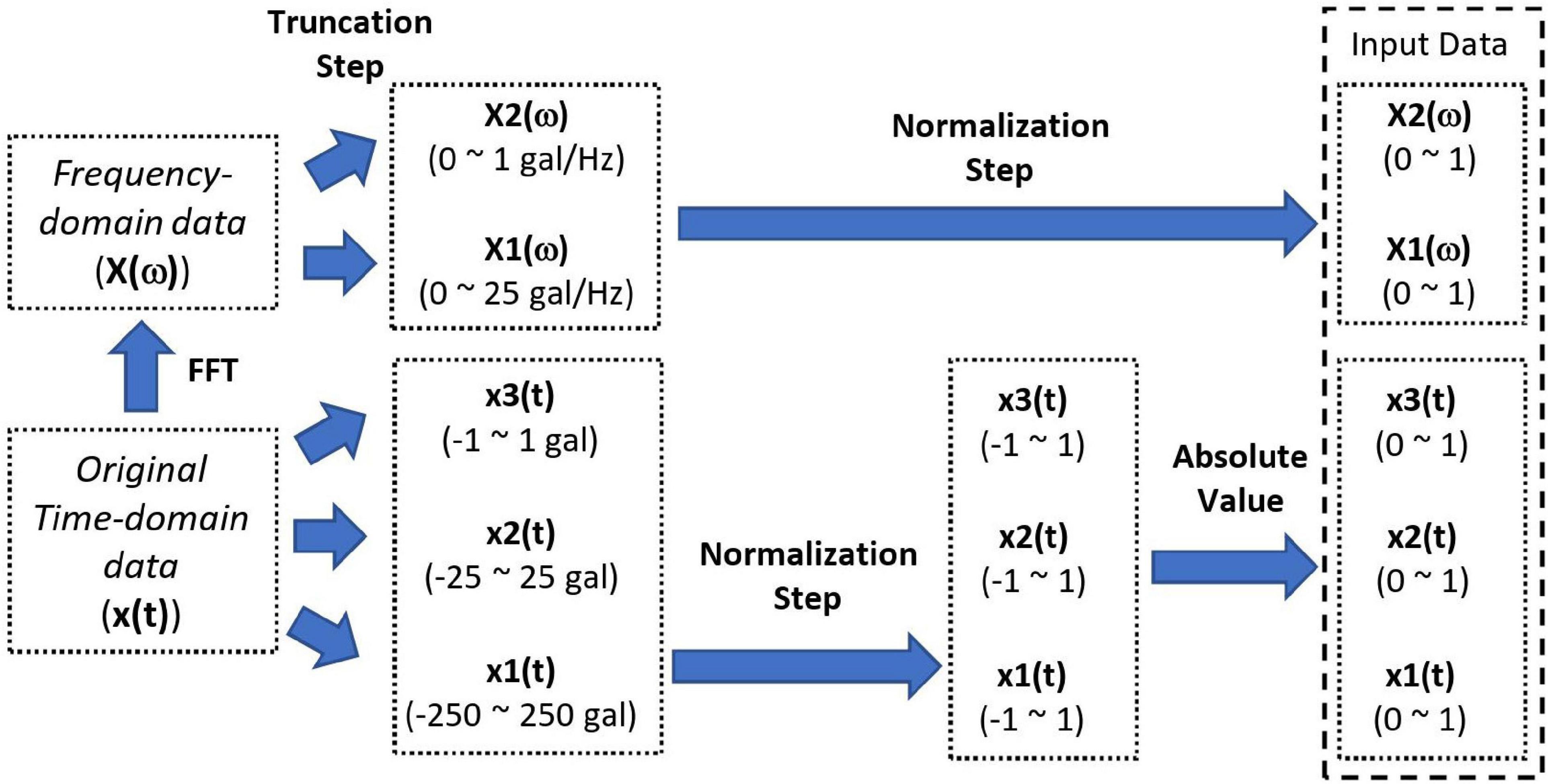
For the first 3 s of the P-wave data in this study, the maximum amplitude of most of the data (99.9%) was below 250 gal (cm/s²). This indicates that one of the scales of time history data could be chosen as ± 250 gal. That is, the original time history data with values larger than 250 gal and smaller than −250 gal were truncated and set to 250 and −250 gal, respectively (Truncation Step). Then the truncated data were rescaled to have values between −1 and 1 (Normalization Step). Four more scales with ranges of ±2.5, ±8, ±25, and ±80 gal were also considered to extract the features of time history data with different amplitudes. These range of scales is referred to the seismic intensity scale of the Central Weather Bureau (CWB), Taiwan. The discussion of determining the scales of time history data are provided in section 3.1 Effect of Input.

It is well-known in the geoscience research community that the seismic ground motions caused by a longer fault-rupture process may contain signals with longer periods (Satriano et al., 2011). This identifies the frequency content of the P-wave as very important. However, because it is not easy to identify the frequency content clearly by observing the complex and chaotic ground acceleration time history directly, the frequency domain of the P-wave data was also included in the input into the CNN. As a result, both the time and frequency domains of the P-wave data are combined as multi-domain input so that the CNN can observe the data in different aspects.

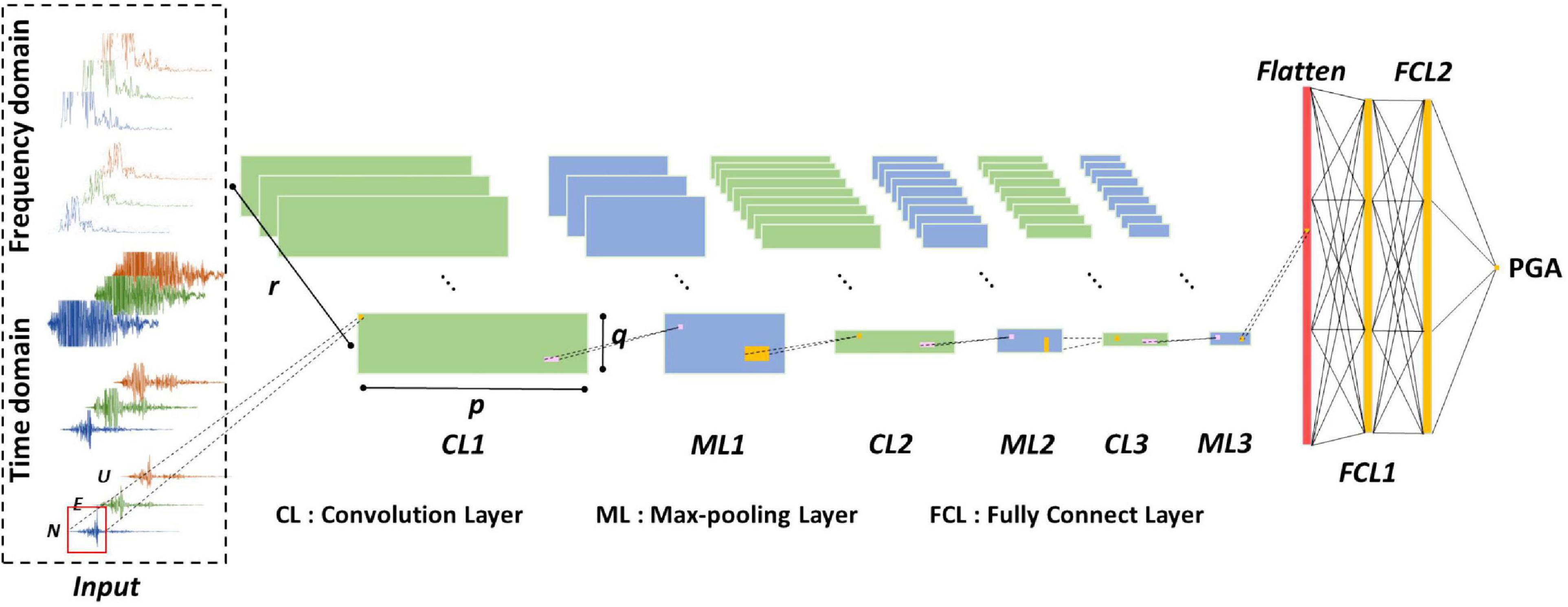
Similar to the time history of the P-wave data, three different scales of the Fourier spectrogram, i.e., 1, 20, and 40 gal/Hz, were also considered in order to observe the frequency content more clearly in different scales using the CNN. The Fourier spectrogram is the amplitude obtained by using fast Fourier transformation of the first 3 s of P-wave data. Take the scale 20 gal/Hz as an example, the original Fourier spectrogram with values larger than 20 gal/Hz was truncated and set to 20 gal/Hz (Truncation Step). Then the truncated data were rescaled to have values between −1 and 1 (Normalization Step). For 3 s of three components’ time history with a 200 Hz sampling rate, the size of each scale of P-wave time history data was 600 × 3. However, because most of the energy of the P-wave data is located within a frequency range between 0 and 50 Hz, only the spectrogram of this range was used (150 points in length). In order to have the same dimensions for both the time and frequency domain data, 600 points, the spectrogram was linearly interpolated. Finally, there were five multi-scale and multi-domain P-wave data as the input of the CNN, as shown in Figure 1, and the dimensions of the input data were 600 × 3 × 5.

FIGURE 1

Figure 1. The proposed CNN architecture in this study.

Architecture of the CNN

It is well known that intensive periodicity may exist in the time-domain vibration signals and the signals at different time points could be deeply related to each other in a large range. Hence, it may be difficult to find valuable information about periodic data and the relationship behind the time history signals by using kernels with short lengths along the time dimension. As for the data in the frequency domain, the relationship between higher and lower frequencies can be extracted using kernels with longer lengths along the frequency dimension. For instance, Yu et al. (2018) successfully identified structural damage using a 1,000 × 1 kernel size for extracting features from frequency spectra along the frequency dimension. In this study, 16 1-D kernels 150 × 1 in size in the first layer were implemented to extract the features of the data for both the time and frequency domains. Then a max pooling layer with 1-D kernels with a size of 3 × 1 and a stride of 3 × 1 was used to extract the maximum value of the features along the time-series direction. Figure 1 shows the architecture of the proposed CNN. The max pooling could greatly improve the statistical efficiency and computational speed of the neural network. The schematic diagrams of the operation of convolution and pooling, as well as the resulting sizes of the feature maps, are shown in Figure 2.

FIGURE 2

Figure 2. The schematic diagram of the operation of convolution and pooling, as well as the resulted size of the feature maps.

After the feature maps were extracted from the time history data and frequency spectra, we treated these feature maps more like 2-D images. Therefore, the second convolution layer with 32 2-D kernels that were 5 × 3 in size and a pooling layer with kernels of 3 × 1 in size were employed to extract more condensed features. And the third convolution layer with 32 kernels 1 × 3 in size and a pooling layer with kernels 3 × 1 in size were employed again to further extract more condensed features.

Finally, after the features were flattened, two fully connected layers of 128 neurons that served as feature-selection layers were utilized to transform the feature maps into the output PGA value, so as most unnecessary or redundant features will be cast aside in the fully connected layers. The details of the sizes of the convolution and pooling operations, as well as the resulted sizes of the feature maps, are summarized in Table 1. The rectified linear unit (ReLU) activation function was employed in this study (Nair and Hinton, 2010), and the dropout operation was applied to avoid over-diffing problems (Srivastava et al., 2014).

TABLE 1

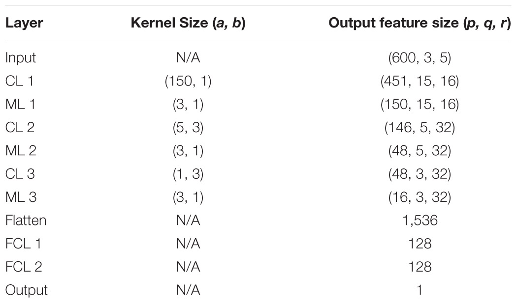
Table 1. The detail of the size of the convolution and pooling operations, as well as the resulting sizes of the feature maps of the proposed CNN.

Earthquake Data

The earthquake data provided by the Taiwan Strong Motion Instrument Program (TSMIP) were employed in this study. High-quality strong ground motions caused by earthquakes around Taiwan were collected by the TSMIP network, which is operated by the CWB. In total, data on 10,000 earthquakes (denoted as T-data) were selected from the TSMIP data covering the period from July 29, 1992, to December 31, 2006. All the earthquake data with PGAs larger than 250 cm/s² (gal) and less than 2.5 gal in the TSMIP data were selected because they are quite rare. As for the earthquake data with PGAs between 2.5 and 250 gal, data on more than 2,000 earthquakes were selected. The number of T-data within different ranges of PGA when performing training, validating and testing for the CNN is summarized in Table 2. For instance, the number of all the data with PGAs larger than 400 gal in the TSMIP data was only 78, and 50, 12, and 16 of these data were used for training, validation, and testing, respectively. The number of events within different ranges of PGA is also summarized in the same table. There were 2,279 earthquake events in the T-data, and the magnitude (Mw) range is 1.66∼7.6. Besides the Chi-Chi earthquake event with a magnitude 7.6, there were also some large earthquake events in the T-data and the number of earthquake events with a magnitude not smaller than 6.5 was 17. The frequency of the magnitude for training, validation, and testing datasets is illustrated in Supplementary Figure 1. The magnitude vs. hypocentral distance of the T-data is shown in Supplementary Figure 2. The Short-Term-Average through Long-Term-Average algorithm was employed herein to pick the arrival time of P-wave automatically, and the T-data were used to train, validate, and test the CNN.

TABLE 2

Table 2. The 10,000 TSMIP earthquake data used for training, validating, and testing for the CNN.

In addition, two earthquake datasets recorded during the 2016 Meinong earthquake event (Mw = 6.53) and 2018 Hualien Earthquake event (Mw = 6.2) in Taiwan were adopted herein to understand the capability of the proposed CNN approach for PGA prediction. The Meinong earthquake event resulted in 117 deaths and damaged to 253 buildings (six totally collapsed). The Hualien earthquake event caused 17 fatalities and caused serious damage to 179 buildings (four totally collapsed). Another typical earthquake dataset recorded during a relatively small earthquake event with magnitude 5.3 Mw occurred in 2016 (denoted as M5.3 earthquake) was also adopted to see how the performance of the proposed CNN approach varies with magnitude. The M5.3 earthquake was selected because of its number of the recorded earthquake data were relatively large among the earthquake events with a magnitude between 5.0 and 5.5.

Training and Validation

The goal of the CNN was to predict the PGAs as accurately as possible for small and large earthquakes. However, the differences between these PGAs were quite enormous. To be more specific, the PGAs of large earthquakes could be almost 1,000 times those of the small ones. When the root mean squared errors was used to estimate the loss of the CNN, only the PGAs of larger earthquakes were predicted with high accuracy because the error of these earthquakes contributed to the root mean squared errors much more than did the small earthquakes. In this study, the root mean squared logarithmic errors (RMSLE) was employed to estimate the loss of the CNN, denoted as E, as defined in Equation (1).

$$E=\sqrt{\frac{1}{N}\sum _{j=1}^N{\left(log(y_j^p+1)-log(y_j^r+1)\right)}^2}(1)$$

where $y_j^r$ and $y_j^p$ were the real and predicted PGA of the j^th earthquake, respectively. N is the total number of earthquakes.

The T-data of each PGA range in Table 2 was randomly split into training (64%), validation (16%), and test (20%) sets. We trained the network on one NVIDIA RTX 2080 GPU. We updated the CNN parameters using the Adam optimizer with β₁ = 0.9, β₂ = 0.999, and decay = 0, and learning rate = 0.001 (Kingma and Ba, 2015). During the train process, the CNN was updated by evaluating and reducing the loss on a batch-by-batch basis with batch size = 32. When the loss of the validation dataset was larger than the one of the training dataset for five epochs successively, the training process was stopped. Supplementary Figure 3 illustrates the typical training process of the CNN.

Results

Effect of Input

In this section, we studied the effects of the input on the PGA predictions using CNN. First, the effects of adding one more scale of P-wave time history data or spectrogram were studied as an initial study to understand if adding one different measure of the input help the PGA prediction or not. The means of the RMSLE of 15 repeated trials of the 2,000 test data of these cases are summarized in Supplementary Table 1. The results of using only a single scale of the P-wave time history, i.e., scale of 250 gal, are also listed in the same table for comparison. The results show that adding one more scale of P-wave time history data or spectrogram reduced the RMSLE values quite a lot, especially when one scale of the spectrogram was included.

Next, the effects of combinations of three different scales of P-wave time history data were studied. These results were also compared to the ones using only a single scale of the P-wave time history data (Case TH1). These are the five scales of P-wave time history data that were considered: 2.5, 8, 25, 80, and 250 gal. In total, one single-scale (Case TH1) and 10 different combinations of these five scales (Case TH2 to TH11) were studied, as listed in Table 3. The box plots of the RMSLE of 15 repeated trials of the 2,000 test data are plotted in Figure 3. Apparently, all the combinations of three different scales of P-wave time history data outperformed the single-scale one. Among the combinations of the three different scales of P-wave time history data, the RMSLE of Case TH5 to TH8 is relatively smaller than the others, as can also be observed from the mean of the RMSLE as listed in Table 3. Nevertheless, these results indicate that combining different scales of P-wave time history data helped the CNN extract more informative features and achieve a better PGA prediction.

TABLE 3

Table 3. The details of the combinations and the RMSLE of cases TH1 to TH11.

FIGURE 3

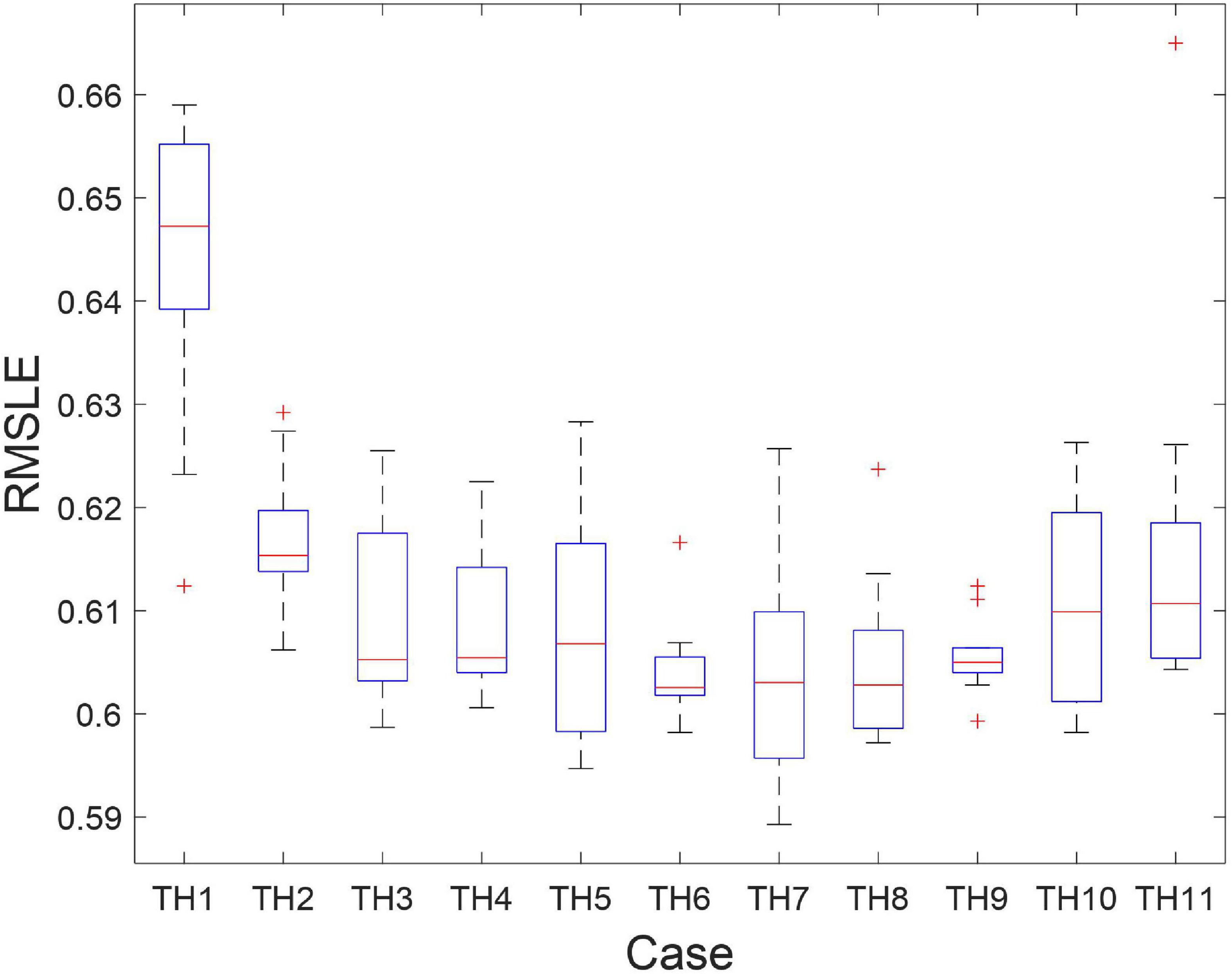
Figure 3. The box plots of the RMSLE of the Cases TH1 to TH11 (using raw values of time history data).

Since only the maximum absolute acceleration value of the entire time history of seismic waves is the target output of the CNN, it is possible the signs of the P-wave time history are not so informative, but the amplitude may already provide the necessary information. Therefore, for the input data of CNN, we tried to replace the raw P-wave time history data of the studied combinations with the absolute ones. The box plots of the RMSLE of 15 repeated trials of the 2,000 test data of these combinations using absolute values are plotted in Figure 4. Again, all of the combinations of the three different scales of P-wave time history data outperformed the single-scale one. Based on these results, taking the absolute value of P-wave time history data seems to help the CNN predict the PGA more accurately because the errors are lower in general, and the mean of the RMSLE of all the 11 cases using absolute values are 0.02∼0.03 smaller than the ones using raw values, as listed in Table 3. Besides, the mean of the RMSLE of Case TH6 (the combinations of 2.5++25+250 scales) was the smallest one. Since both the mean and the box plot of the RMSLE of Case TH6 outperforms the others, the combination of 2.5 + 25 + 250 scales using absolute values was selected.

FIGURE 4

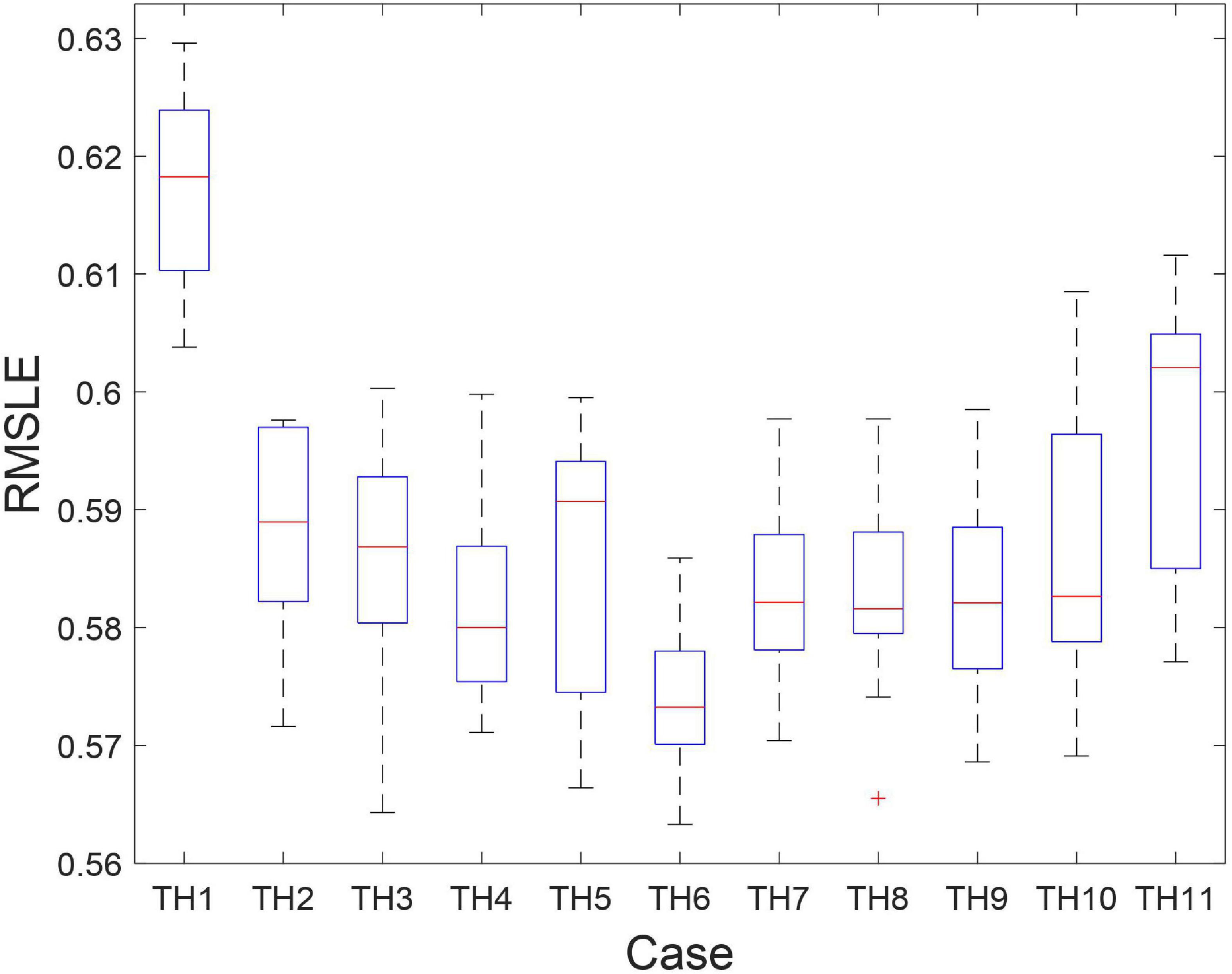
Figure 4. The box plots of the RMSLE of the Cases TH1 to TH11 (using absolute values of time history data).

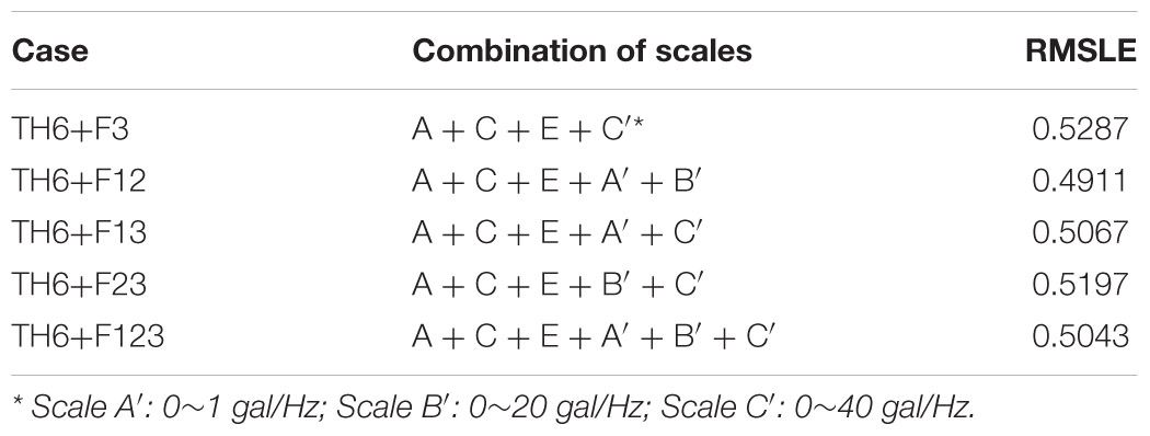
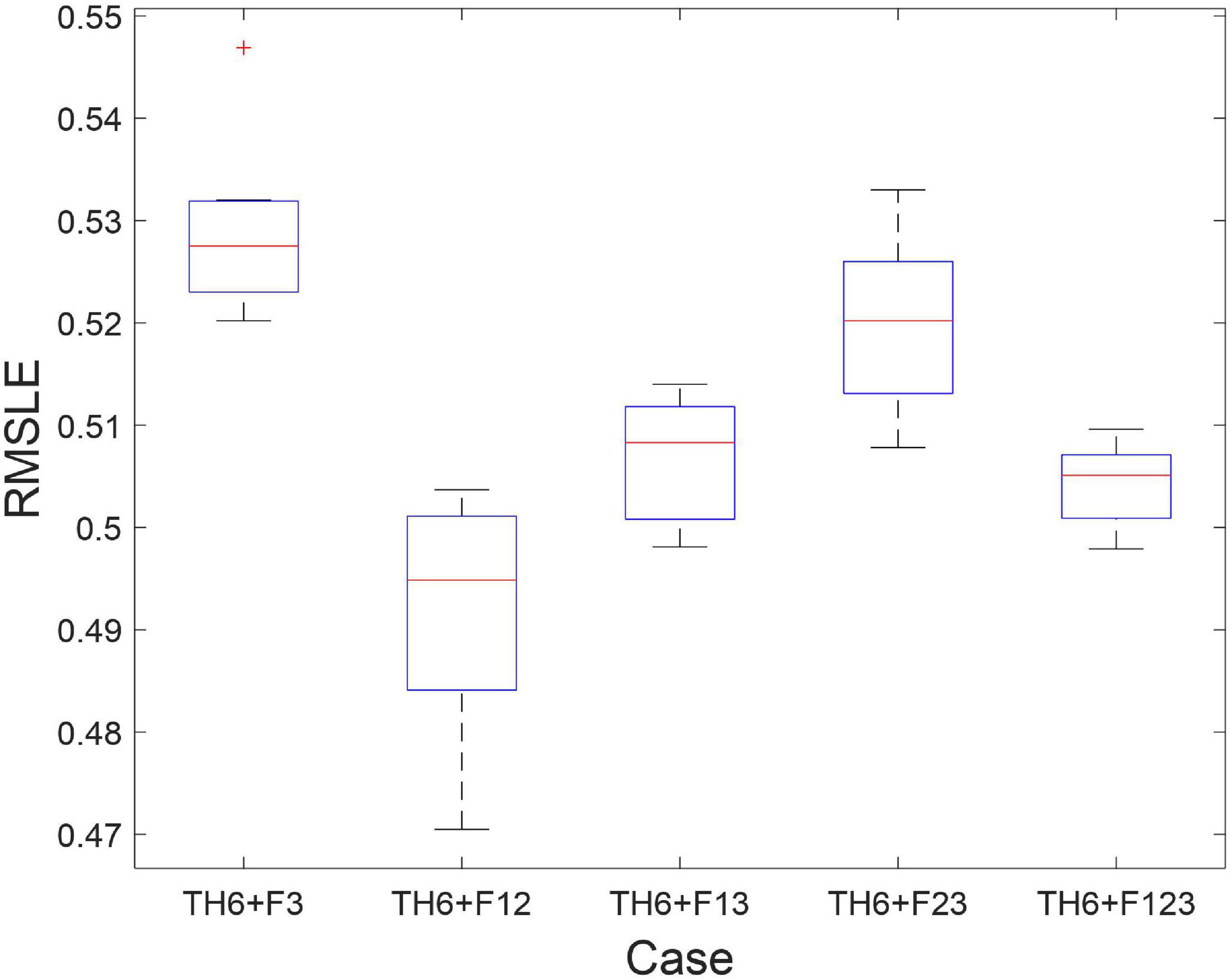
Next, the effects of including a spectrogram on the PGA prediction using CNN were studied. Because the range of the spectrogram amplitude of small and large earthquakes was not as large as the range of the time histories’ amplitudes, only three scales of the spectrogram were considered herein: 0∼1, 0∼20, and 0∼40 gal/Hz. In total, five combinations of the best studied combinations of three different scales of P-wave time history data (Case TH6), and the three scales of the spectrogram were studied as listed in Table 4: cases TH6+F3, TH6+F12, TH6+F13, TH6+F23, and TH6+F123. The box plots of the RMSLE of 15 repeated trials of the 2,000 test data are plotted in Figure 5. It is evident that including the spectrogram can achieve much smaller RMSLE values than the one without any spectrogram. These results indicate that combining the frequency domain with the time domain P-wave data helped the CNN understand more deeply the P-wave data for PGA prediction. Among the five cases, case TH6+F12, which includes the smallest two scales of the spectrogram, has the smallest RMSLE value, as can also be observed in Table 4, hence it should be employed in future studies. Finally, the procedures to obtain the multi-domain and multi-scale input for the CNN as described previously are summarized in Figure 6.

TABLE 4

Table 4. The details and RMSLE of the combinations of cases TH6+F3 to TH6+F123.

FIGURE 5

Figure 5. The box plots of the RMSLE of the Cases TH6+F3 to TH6+F123.

FIGURE 6

Figure 6. The summarized procedures to obtain the multi-domain and multi-scale input for the CNN.

Results of the T-Data

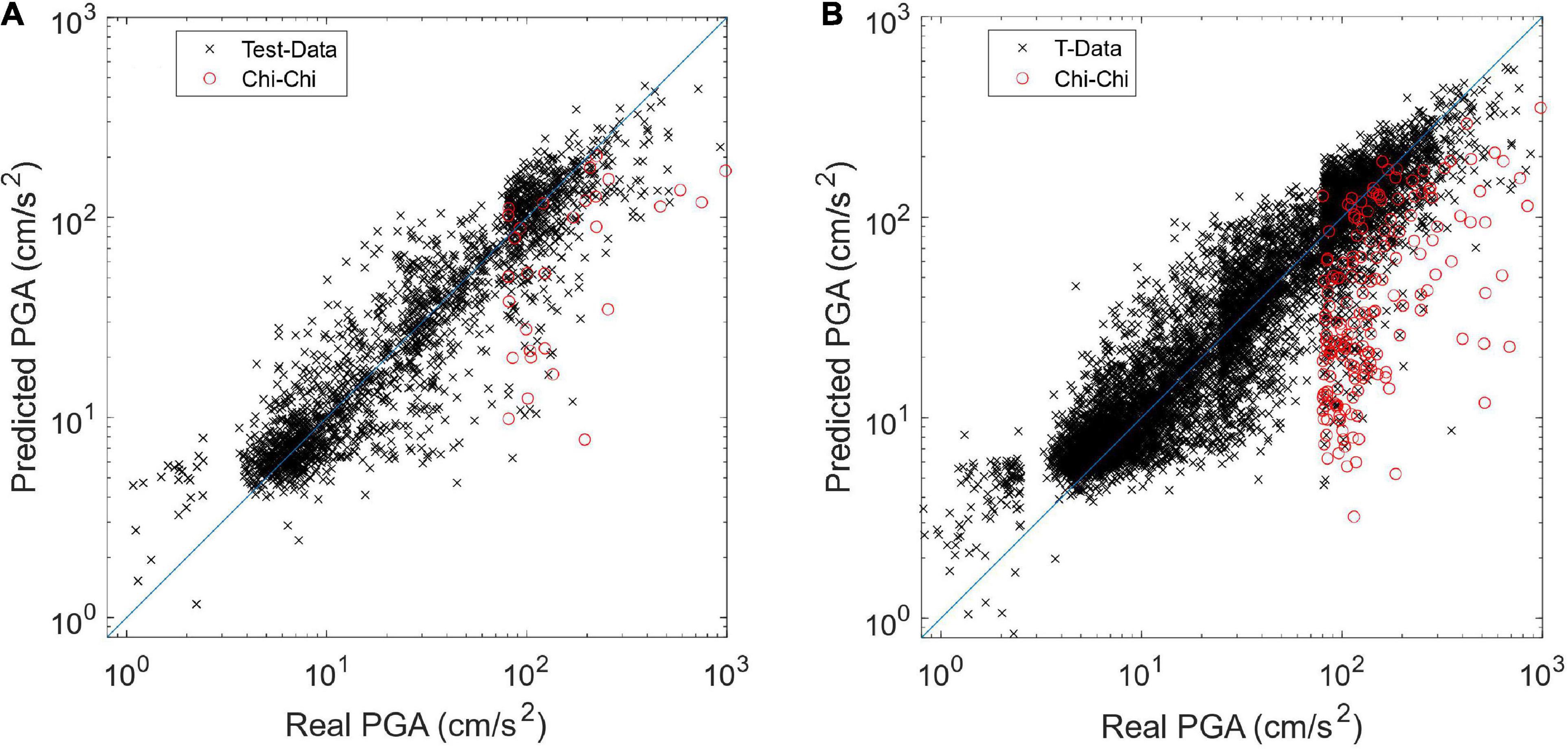
Based on the results of the input study, we took case TH6+F12, which has three scales of the absolute value of the P-wave time history data and two scales of the Fourier spectrograms of the original value of the P-wave data, as the final input of the CNN used in this study. The predicted PGA distribution of the 2,000 test data is illustrated in Figure 7A. Besides, the predicted PGA distribution of all 10,000 T-data is illustrated in Figure 7B. Apparently, the PGA distributions of the test data and all the T-data are quite similar. The RMSLE of all the T-data was still quite small at 0.454, which indicates that overfitting had not occurred. For easier comparison to other approaches, the standard variation (σ) of the errors between the predicted and real PGAs in natural logarithmic scale of all the T-data was also calculated, and its value was 0.512.

FIGURE 7

Figure 7. The predicted PGA distribution of (A) the 2,000 test data and (B) all the 10,000 T-data.

The PGA distribution using the best combination, case TH6+F12, can be found in Figure 7. Despite most of the predicted PGAs being quite close to the real PGAs, there are still some earthquakes with larger real PGAs that are apparently underestimated (e.g., a PGA greater than 80 gal). These earthquakes actually belong to the Chi-Chi earthquake event on September 21, 1999, as marked in Figure 7 and separately illustrated in Figure 8A. This is mainly because only the first few seconds of P-wave data is employed to predict PGA, but the Chi-Chi earthquake event had at least two asperities, which makes the slip propagation process quite long and complex (Ma et al., 2001). More specifically, the Chi-Chi earthquake intensity was predominantly contributed by the major asperity rupture 13 s after another minor one, making the PGA prediction based on the first few seconds of the P-wave harder. Hsu et al. (2013) has illustrated the PGA can be predicted much closer to the real PGA if the information of the longer P-wave data is used. More details about the discussion the PGA prediction of the Chi-Chi earthquake event using the SVR approach are in Hsu et al. (2013). Herein, the PGA prediction results using the SVR approach with the same first 3 s of time history after the triggering of the Chi-Chi earthquake are illustrated in Figure 8B for comparison. The RMSLE of the Chi-Chi earthquake using the proposed CNN and the SVR approaches was 1.419 and 1.867, respectively. Evidently, the proposed CNN approach can predict the PGAs of these earthquakes more accurately than the SVR approach.

FIGURE 8

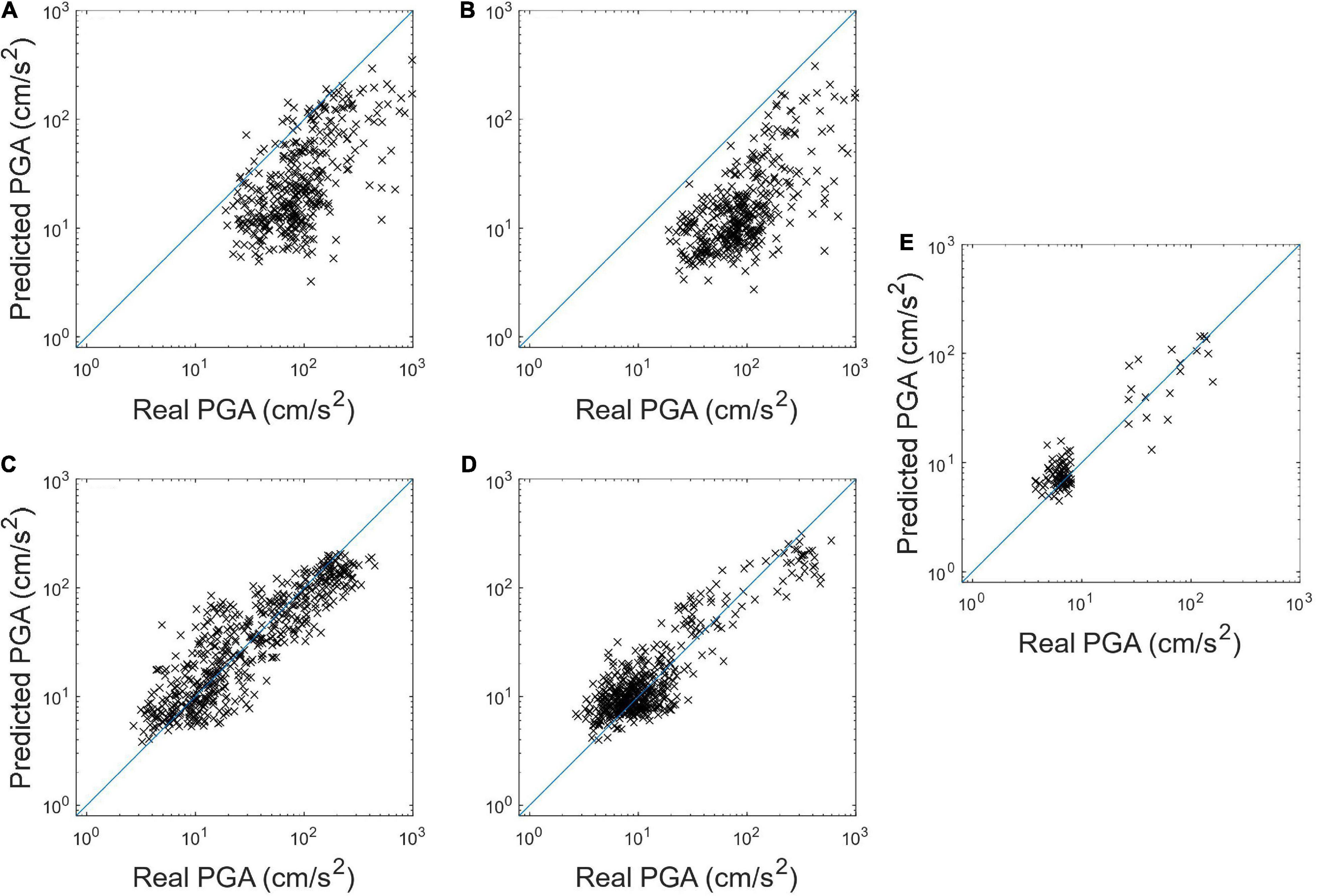
Figure 8. The predicted PGA distribution of the Chi-Chi earthquake event using (A) the proposed CNN approach and (B) the SVR approach in Hsu et al. (2013). The predicted PGA distribution of (C) the Meinong earthquakes, (D) the Hualien earthquakes, and (E) the M5.3 earthquake using the proposed CNN approach.

Results of the Test Earthquakes

In addition to the T-data, we tested the performance of the proposed CNN approach using the independent 2016 Meinong earthquake event and the 2018 Hualien earthquake event. The predicted PGA distribution of these two earthquake events are illustrated in Figures 8C,D. The RMSLE of the Meinong and Hualien earthquake events are 0.561 and 0.476, respectively. It seems the proposed CNN can, in general, predict the PGAs of separate damaging earthquake events with anticipated accuracy. Besides, in order to understand the performance of PGA prediction using the CNN approach during a typical earthquake event with a smaller magnitude (between 5 and 5.5), the predicted PGA distribution during the M5.3 earthquake is illustrated in Figure 8E. The RMSLE of the PGA prediction results of the M5.3 event is only 0.378. It seems the proposed CNN approach can predict the PGAs of the typical earthquake event with a smaller magnitude quite well. For easier comparison to other approaches, the standard variation (σ) of the errors between the predicted and real PGAs in natural logarithmic scale of these three test earthquake events and the Chi-Chi earthquake event was also listed in Table 5.

TABLE 5

Table 5. The summary of the metrics of the proposed CNN.

To further understand the potential alert performance using the proposed CNN of these two earthquake events, the confusion matrix was employed herein. The threshold was set to 25 gal, which is identical to the one used in the onsite EEW algorithm of the EEW System of the National Center for Research on Earthquake Engineering, Taiwan (NEEWS) during these two earthquake events (Hsu et al., 2016, 2018). In order to focus on the discussion of the accuracy of the predicted PGAs, the lead-time of all the earthquakes was assumed as valid. As a result, as summarized in the confusion matrix of Figure 9A, if both the predicted PGA and the real PGA are ≥25 gal, we considered this result a true positive (“TP”). Conversely, if the predicted PGA is ≥25 gal, but the real PGA never reached the threshold, we considered this result a false positive (“FP”). If both the predicted PGA and the real PGA are <25 gal, we considered this result a true negative (“TN”). If the final ground motion amplitude reached the threshold, but the predicted PGA did not, then we considered this result a false negative (“FN”). The performance metrics based on the confusion matrix, such as F1-score, precision, and recall are shown in Table 5.

FIGURE 9

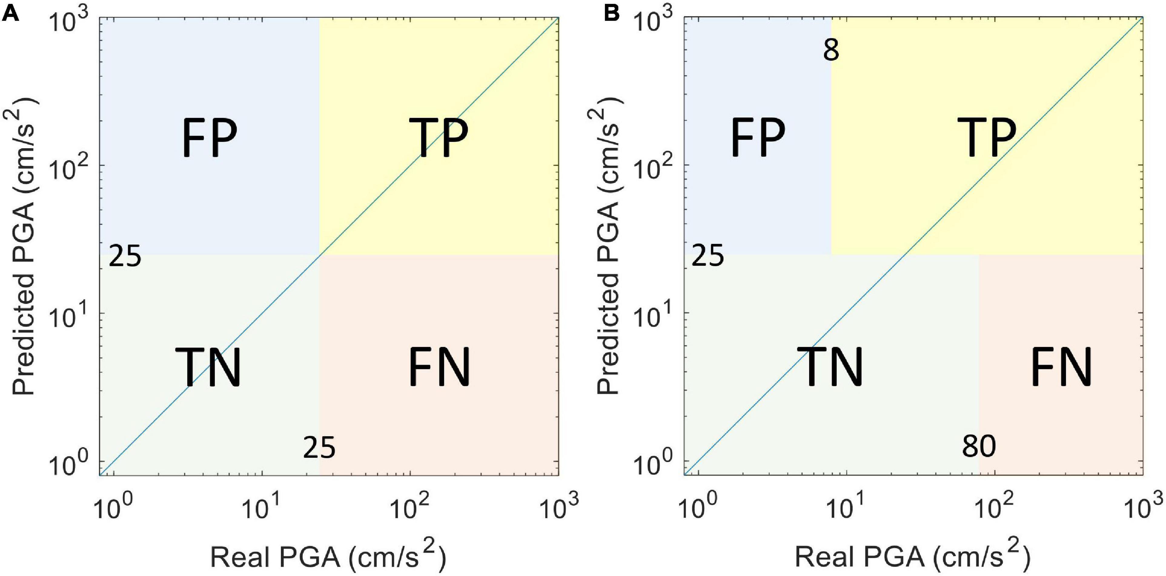
Figure 9. The confusion matrix (A) without a classification tolerance and (B) with a classification tolerance range of ± 1 level of CWB intensity scale.

As proposed by Meier (2017), to evaluate the classification performance of the EEW system, a tolerance range can be used. We use the same tolerance as the NEEWS (Hsu et al., 2018) during these three earthquake events, i.e., a ± 1 level of CWB intensity scale, to evaluate the performance of the proposed CNN herein, as shown in Figure 9B. The performance metrics based on the confusion matrix with a tolerance are also summarized in Table 5. The values of the precision, recall, and F1-score when no tolerance is allowed are approximately between 81% and 100%, while the ones when the tolerance is allowed increased to approximately at least 97%. Hence in general, the overall potential alert performance using the proposed CNN during these three test earthquake events seems quite promising.

In Comparison With the SVR and GMPE-Based Approaches

As described in the Introduction section, the SVR approach developed previously has been employed in the NEEWS in Taiwan and has successfully demonstrated its ability during several damaging earthquakes. Six P-wave features are extracted from the first 3 s of the vertical acceleration and then used as the input to the SVR prediction model for PGA prediction. The same T-data were used herein to know if the predicted PGA of the proposed CNN is more accurate than the one using the SVR or not. The PGA distributions of the T-data earthquakes using the SVR prediction model of the NEEWS are illustrated in Figure 10A, with the RMSLE and σ value equal to 0.748 and 0.664, respectively. These values are much larger than the ones using the proposed CNN approach. These results indicate the superiority of the CNN for PGA prediction.

FIGURE 10

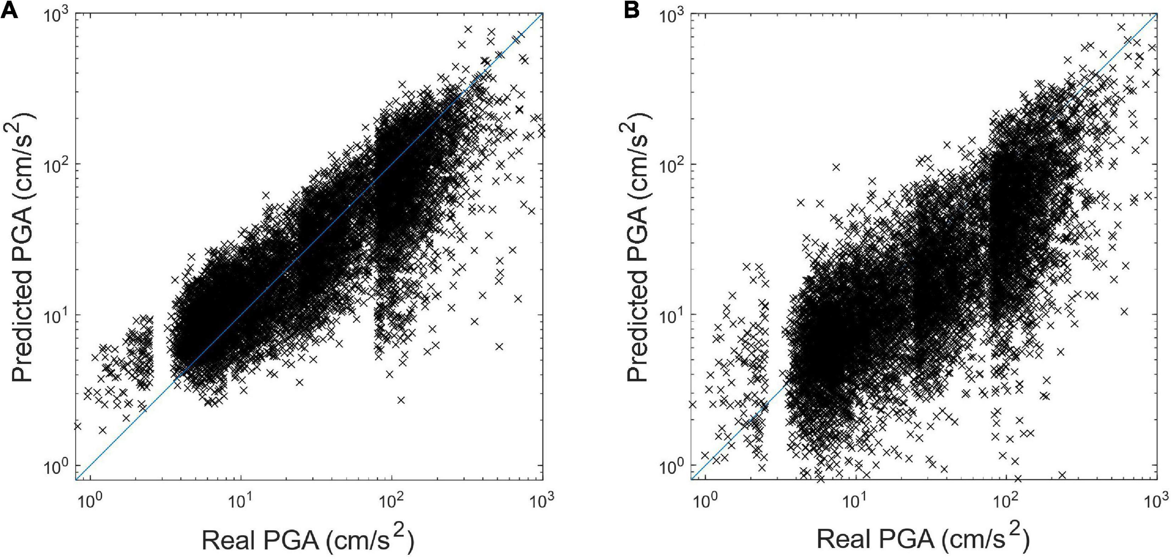
Figure 10. The predicted PGA distribution of the 10,000 T-data earthquakes using (A) the SVR approach in Hsu et al. (2013), and (B) the GMPE-based approach.

Many EEW systems around the world use a ground motion prediction equation (GMPE) to forecast shaking based on estimates of the source parameters (location and magnitude). For comparison, under the assumption that the location and magnitude could be accurately estimated, the PGA could be predicted based on the GMPE. The GMPE accommodating site effects developed by Jean et al. (2006) was employed herein and the same T-data were used to compare the proposed CNN with the typical GMPE-based approach. The PGA distributions of the T-data earthquakes using the GMPE-based approach are illustrated in Figure 10B, with the RMSLE and σ value equal to 0.870 and 0.896, respectively. Again, these values are much larger than the ones using the proposed CNN approach, which indicates the accuracy of the CNN for PGA prediction is quite promising.

Discussion

In this study, the CNN is proposed as having successfully predicted the PGA of the incoming seismic wave at the same site based on the information of the first 3 s of P-wave data after an event is triggered. Due to this specific application to EEW, the proposed CNN is specially designed. The novel multi-scale input of the CNN is proposed to deal with the enormous differences of the amplitudes of the input data. The multi-domain information of the P-wave data (both the time history and Fourier spectrogram) is also proposed as helping to achieve better PGA prediction accuracy for the CNN. The multi-scale and multi-domain input data are treated as different aspects of the P-wave data. Moreover, the absolute value of the time history data is employed when input to the CNN, instead of the raw one, since only the maximum absolute acceleration value of the coming seismic wave is needed to be predicted for the CNN. Note that we aim to propose using the combination of different scales of both the P-wave time history data and spectrogram, but not to propose the best combination of that. Therefore, not all the possible combinations were considered in this study.

The proposed arrangement of the input data shows its superiority to the one directly inputting the raw P-wave data into the CNN. In addition, the proposed CNN approach also shows its superiority for PGA prediction without extracting any P-wave features in advance to the SVR approach employed by the NEEWS where P-wave features must be extracted in advance.

Two independent damaging earthquake events that occurred recently in Taiwan were employed to understand the capability of the proposed CNN. The results show the accuracy of the predicted PGAs of these earthquakes are quite acceptable. The potential alert performance using the proposed CNN under the assumption that the lead-time of all the earthquakes were valid was also studied. The F1-score of the proposed CNN during these two damaging earthquake events was approximately 93.4% and increased to approximately 98.8% if the tolerance of ± 1 level of CWB intensity scale was acceptable. Besides, the proposed CNN also shows its performance during a typical smaller earthquake event (Mw = 5.3) could be also quite promising.

Based on the results of the T-data and the three test earthquake events, the proposed CNN approach seems quite promising for PGA prediction. However, for the Chi-Chi earthquake event with a long and complex slip propagation process, using only the first few seconds of P-wave data for PGA prediction is still very difficult. This limitation of the proposed CNN approach has been pointed out, and further studies are still required to develop a PGA prediction model for such an earthquake event. One of the possible approaches is to train multiple CNNs for longer durations and change to different ones as the earthquake progresses for better PGA prediction; however, the response time will be sacrificed, as discussed in Hsu et al. (2013) using the SVR approach.

The SVR approach and the proposed CNN approach use seismic wave measured at one seismic station and predict the coming peak ground shaking of the same station. On the other hand, the GMPE-based approach forecast shaking based on estimates of the source parameters. Based on the experience of two real earthquake events, the accuracy of the predicted PGAs of SVR and GMPE-based approaches was quite similar, but the SVR approach could provide a longer lead time for near-epicentral sites (Hsu et al., 2018, 2021). We believe the CNN approach would show similar performance to the SVR approach because their computation time is similar. There are other approaches that use shaking to directly predict shaking, such as the propagation of local undamped motion (PLUM) and the approximation by local pseudo-hypocenter attenuation (ALPHA) approaches developed by the JMA (Kodera et al., 2018; Kodera, 2019). Based on the results of the first-year performance of the PLUM approach, this kind of approach seems to have great potential to provide a more accurate prediction of ground motion intensity and a longer lead time than the GMPE-based approach, especially for destructive earthquakes. However, it is still difficult to provide timely ground motion predictions for near-epicentral sites. Nevertheless, more researches on the performance, comparison, and combination of different EEW approaches are necessary in the future in order to provide better EEW for the public.

Data Availability Statement

The original contributions presented in the study are included in the article/Supplementary Material, further inquiries can be directed to the corresponding author/s.

Author Contributions

T-YH designed the research study and wrote sections of the manuscript. C-WH constructed the CNN and ran the analysis. Both authors contributed to the article and approved the submitted version.

Funding

This research is partially supported by the Taiwan Building Technology Center from The Featured Areas Research Center Program within the framework of the Higher Education Sprout Project by the Ministry of Education in Taiwan.

Conflict of Interest

The authors declare that the research was conducted in the absence of any commercial or financial relationships that could be construed as a potential conflict of interest.

Acknowledgments

The authors would like to thank the Taiwan Strong Motion Instrument Program operated by Central Weather Bureau (CWB) in Taiwan for providing high-quality strong ground motions caused by earthquakes around Taiwan.

Supplementary Material

The Supplementary Material for this article can be found online at: https://www.frontiersin.org/articles/10.3389/feart.2021.626908/full#supplementary-material

References

Abdel-Hamid, O., Mohamed, A., Jiang, H., Deng, L., Penn, G., and Yu, D. (2014). Convolutional neural networks for speech recognition. IEEE/ACM Trans. Audio Speech Lang. Process. 22, 1533–1545.

Google Scholar

Allen, R. M., and Melgar, D. (2019). Earthquake early warning: advances, scientific challenges, and societal needs. Annu. Rev. Earth Planet. Sci. 47, 361–388. doi: 10.1146/annurev-earth-053018-060457

CrossRef Full Text | Google Scholar

Böse, M., Heaton, T., and Hauksson, E. (2012). Rapid Estimation of earthquake source and ground-motion parameters for earthquake early warning using data from a single three-component broadband or strong-motion sensor. Bull. Seismol. Soc. Am. 102, 738–750. doi: 10.1785/0120110152

CrossRef Full Text | Google Scholar

Cuéllar, A., Espinosa-Aranda, J. M., Suarez, R., Ibarrola, G., and Uribe, A. (2014). “The Mexican seismic alert system (SASMEX): its alert signals, broadcast results and performance during the M 7.4 Punta Maldonado earthquake of March 20th, 2012,” in Early Warning for Geological Disasters, eds F. Wenzel and Z. Zschau (Berlin: Springer-Verlag), 71–87. doi: 10.1007/978-3-642-12233-0_4

CrossRef Full Text | Google Scholar

Cui, Z., Chen, W., and Chen, Y. (2016). Multi-scale convolutional neural networks for time series classification. arXiv [Preprint] arXiv: 1603.06995,Google Scholar

Fujinawa, Y., and Noda, Y. (2013). Japan’s earthquake early warning system on 11 March 2011: performance, shortcomings, and changes. Earthq. Spectra 29, S341–S368.

Google Scholar

Hsu, T. Y., Huang, S. K., Chang, Y. W., Kuo, C. H., Lin, C. M., Chang, T. M., et al. (2013). Rapid on-site peak ground acceleration estimation based on support vector regression and P-wave features in Taiwan. Soil Dyn. Earthq. Eng. 49, 210–217. doi: 10.1016/j.soildyn.2013.03.001

CrossRef Full Text | Google Scholar

Hsu, T. Y., Kuo, C. H., Wang, H. H., Chang, Y. W., Lin, P. Y., and Wen, K. L. (2021). The realization of an earthquake early warning system for schools and its performance during the 2019 ML 6.3 Hualien (Taiwan) earthquake. Seismol. Res. Lett. 92, 342–351. doi: 10.1785/0220190329

CrossRef Full Text | Google Scholar

Hsu, T. Y., Lin, P. Y., Wang, H. H., Chiang, H. W., Chang, Y. W., and Kuo, C. H. (2018). Comparing the performance of the NEEWS earthquake early warning system against the CWB system during the 6 February 2018 Mw 6.2 Hualien earthquake. Geophys. Res. Lett. 45, 6001–6007.

Google Scholar

Hsu, T. Y., Wang, H. H., Lin, P. Y., Lin, C. M., Kuo, C. H., and Wen, K. L. (2016). Performance of the NCREE’s on-site warning system during the 5 February 2016 Mw 6.53 Meinong earthquake. Geophys. Res. Lett. 43, 8954–8959. doi: 10.1002/2016gl069372

CrossRef Full Text | Google Scholar

Hsu, T. Y., Wu, R. T., Liang, C. W., Kuo, C. H., and Lin, C. M. (2020). Peak ground acceleration estimation using P-wave parameters and horizontal-to-vertical spectral ratios. Terr. Atmos. Ocean. Sci. 31, 1–8. doi: 10.3319/tao.2019.07.04.01

CrossRef Full Text | Google Scholar

Jean, W. Y., Chang, Y. W., Wen, K. L., and Loh, C. H. (2006). Early estimation of seismic hazard for strong earthquakes in Taiwan. Nat. Hazards 37, 39–53. doi: 10.1007/s11069-005-4655-y

CrossRef Full Text | Google Scholar

Jozinovic, D., Lomax, A., Stajduhar, I., and Michelini, A. (2020). Rapid prediction of earthquake ground shaking intensity using raw waveform data and a convolutional neural network. Geophys. J. Int. 222, 1379–1389. doi: 10.1093/gji/ggaa233

CrossRef Full Text | Google Scholar

Kanamori, H. (2005). Real-time seismology and earthquake damage mitigation. Annu. Rev. Earth Planet. Sci. 33, 195–214. doi: 10.1146/annurev.earth.33.092203.122626

CrossRef Full Text | Google Scholar

Kingma, D. P., and Ba, J. (2015). “Adam: a method for stochastic optimization,” in Proceedings of the 3rd International Conference on Learning Representations (ICLR), Conference Track Proceedings, San Diego, CA.

Google Scholar

Kodera, Y. (2019). An earthquake early warning method based on Huygens principle: Robust ground motion prediction using various localized distance-attenuation models. J. Geophys. Res. 124, 12981–12996. doi: 10.1029/2019jb017862

CrossRef Full Text | Google Scholar

Kodera, Y., Saitou, J., Hayashimoto, N., Adachi, S., Morimoto, M., Nishimae, Y., et al. (2016). Earthquake early warning for the 2016 Kumamoto earthquake: performance evaluation of the current system and the next-generation methods of the Japan meteorological agency. Earth Planets Space 68:202.

Google Scholar

Kodera, Y., Yamada, Y., Hirano, K., Tamaribuchi, K., Adachi, S., Hayashimoto, N., et al. (2018). The propagation of local undamped motion (PLUM) method: a simple and robust seismic wavefield estimation approach for earthquake early warning. Bull. Seismol. Soc. Am. 108, 983–1003. doi: 10.1785/0120170085

CrossRef Full Text | Google Scholar

LeCun, Y., Bengio, Y., and Hinton, G. (2015). Deep learning. Nature 521, 436–444.

Google Scholar

Ma, K. F., Mori, J., Lee, S. J., and Yu, S. B. (2001). Spatial and temporal distribution of slip for the 1999 Chi-Chi, Taiwan, earthquake. Bull. Seismol. Soc. Am. 91, 1069–1087. doi: 10.1785/0120000728

CrossRef Full Text | Google Scholar

Meier, M. A. (2017). How “good” are real-time ground motion predictions from earthquake early warning systems? J. Geophys. Res. Solid Earth 122, 5561–5577. doi: 10.1002/2017jb014025

CrossRef Full Text | Google Scholar

Mousavi, S. M., Zhu, W., Sheng, Y., and Beroza, G. C. (2019). CRED: a deep residual network of convolutional and recurrent units for earthquake signal detection. Sci. Rep. 9:10267.

Google Scholar

Nair, V., and Hinton, G. E. (2010). “Rectifed linear units improve restricted boltzmann machines,” in Proceedings of the 27th International Conference on International Conference on Machine Learning, ICML’10, (Madison, WI: Omnipress), 807–814.

Google Scholar

Nakamura, Y., Saita, J., and Sato, T. (2011). On an earthquake early warning system (EEW) and its applications. Soil Dyn. Earthq. Eng. 31, 127–136. doi: 10.1016/j.soildyn.2010.04.012

CrossRef Full Text | Google Scholar

Odaka, T., Ashiya, K., Tsukada, S., Sato, S., Ohtake, K., and Nozaka, D. (2003). A new method of quickly estimating epicentral distance and magnitude from a single seismic record. Bull. Seismol. Soc. Am. 93, 526–532. doi: 10.1785/0120020008

CrossRef Full Text | Google Scholar

Perol, T., Gharbi, M., and Denolle, M. (2018). Convolutional neural network for earthquake detection and location. Sci. Adv. 4:e1700578. doi: 10.1126/sciadv.1700578

PubMed Abstract | CrossRef Full Text | Google Scholar

Sajjad, M., Khan, S., Hussain, T., Muhammad, K., Sangaiah, A. K., and Castiglione, A. (2018). CNN-based anti-spoofing two-tier multi-factor authentication system. Pattern Recognit. Lett. 126, 123–131. doi: 10.1016/j.patrec.2018.02.015

CrossRef Full Text | Google Scholar

Satriano, C., Wu, Y. M., Zollo, A., and Kanamori, H. (2011). Earthquake early warning: concepts, methods and physical grounds. Soil Dyn. Earthq. Eng. 31, 106–118. doi: 10.1016/j.soildyn.2010.07.007

CrossRef Full Text | Google Scholar

Shrestha, A., and Dang, J. (2020). Deep learning-based real-time auto classification of smartphone measured bridge vibration data. Sensors 20:2710. doi: 10.3390/s20092710

PubMed Abstract | CrossRef Full Text | Google Scholar

Silver, D., Huang, A., Maddison, C., Guez, A., Sifre, L., van den Driessche, G., et al. (2016). Mastering the game of Go with deep neural networks and tree search. Nature 529, 484–489. doi: 10.1038/nature16961

PubMed Abstract | CrossRef Full Text | Google Scholar

Srivastava, N., Hinton, G., Krizhevsky, A., Sutskever, I., and Salakhutdinov, R. (2014). Dropout: a simple way to prevent neural networks from overfitting. J. Mach. Learn. Res. 15, 1929–1958.

Google Scholar

Wu, R. T., and Jahanshahi, M. R. (2019). Deep convolutional neural network for structural dynamic response estimation and system identification. J. Eng. Mech. 145:04018125. doi: 10.1061/(asce)em.1943-7889.0001556

PubMed Abstract | CrossRef Full Text | Google Scholar

Wu, Y. M., and Kanamori, H. (2005). Rapid assessment of damaging potential of earthquakes in Taiwan from the beginning of P waves. Bull. Seismical Soc. Am. 95, 1181–1185. doi: 10.1785/0120040193

CrossRef Full Text | Google Scholar

Wu, Y. M., Mittal, H., Huang, T. C., Yang, B. M., Jan, J. C., and Chen, S. K. (2019). Performance of a low-cost earthquake early warning system (P-Alert) and Shake Map production during the 2018 Mw 6.4 Hualien, Taiwan, earthquake. Seismol. Res. Lett. 90, 19–29. doi: 10.1785/0220180170

CrossRef Full Text | Google Scholar

Xu, Y., Wei, S., Bao, Y., and Li, H. (2019). Automatic seismic damage identification of reinforced concrete columns from images by a region-based deep convolutional neural network. Struct. Control Health Monit. 26:e2313. doi: 10.1002/stc.2313

CrossRef Full Text | Google Scholar

Yamada, M., Tamaribuchi, K., and Wu, S. (2014). Faster and more accurate earthquake early warning system–combination of velocity and acceleration-type seismometers. J. Japan Assoc. Earthq. Eng. 14-4, 21–34. 2014.8. (in Japanese), doi: 10.1007/978-3-540-72241-0_3

CrossRef Full Text | Google Scholar

Yu, Y., Wang, C., Gu, X., and Li, J. (2018). A novel deep learning-based method for damage identification of smart building structures. Struct. Health Monit. 18, 1–21.

Google Scholar

Zollo, A., Amoroso, O., Lancieri, M., Wu, Y. M., and Kanamori, H. (2010). A threshold-based earthquake early warning using dense accelerometer networks. Geophys. J. Int. 183, 963–974. doi: 10.1111/j.1365-246x.2010.04765.x

CrossRef Full Text | Google Scholar