The 2011–2014 Pollino Seismic Swarm: Complex Fault Systems Imaged by 1D Refined Location and Shear Wave Splitting Analysis at the Apennines–Calabrian Arc Boundary

In the years between 2011 and 2014, at the edge between the Apennines collapsing chain and the subducting Calabrian arc, intense seismic swarms occurred in the Pollino mountain belt. In this key region, <2.5 mm/yr of NE-trending extension is accommodated on an intricate network of normal faults, having almost the same direction as the mountain belt. The long-lasting seismic release consisted of different swarm episodes, where the strongest event coinciding with a M_L 5.0 shock occurred in October 2012. This latter comes after a M_L four nucleated in May 2012 and followed by aseismic slip episodes. In this study, we present accurate relocations for ∼6,000 earthquakes and shear-wave splitting analysis for ∼22,600 event-station pairs. The seismicity distribution delineates two main clusters around the major shocks: in the north-western area, where the M_L 5.0 occurred, the hypocenters are localized in a ball-shaped volume of seismicity without defining any planar distribution, whilst in the eastern area, where the M_L 4.3 nucleates, the hypocenters define several faults of a complex system of thrusts and back-thrusts. This different behavior is also imaged by the anisotropic parameters results: a strong variability of fast directions is observed in the western sector, while stable orientations are visible in the eastern cluster. This tectonic system possibly formed as a positive flower structure but as of today, it accommodates stress on normal faults. The deep structure imaged by refined locations is overall consistent with the complex fault system recently mapped at the surface and with patterns of crustal anisotropy depicting fractures alignment at depth. The possible reactivation of inherited structures supports the important role of the Pollino fault as a composite wrench fault system along which, in the lower Pleistocene, the southward retreat of the ionian slab was accommodated; in this contest, the inversion of the faults kinematics indicates a probable southward shift of the slab edge. This interpretation may help to comprehend the physical mechanisms behind the seismic swarms of the region and defining the seismic hazard of the Pollino range: nowadays a region of high seismic hazard although no strong earthquakes are present in the historical record.

Introduction

In a long period between 2011 and 2014, intense seismic swarms developed at the edge between the Calabrian Arc and the Apennines (Govoni et al., 2013; Passarelli et al., 2015).

This area is a crucial node at the rim of the ionian subduction (Totaro et al., 2014; Chiarabba et al., 2016; Palano et al., 2017). Pollino massif has been retained as the major seismic gap (Figure 1C) of peninsular Italy (Locati et al., 2016). The lack of large events (M_W ≥ 6.5) in historical catalogs for a 100 km-long section concurred with this hypothesis in a framework of a unique and continuous seismic belt first introduced by the pioneering intuition of Omori (1909). Therefore, seismic unrest of past years became a great concern for the management of short-term hazard.

FIGURE 1

FIGURE 1. (A) Detailed map of active faults, in the Calabria-Basilicata border region (modified after Brozzetti et al., 2017) and their interaction with Pollino 2010–2014 swarm strongest events. Major structures are represented by: Coastal Range Fault Set (CRFS); Castello Seluci-Viggianello-Piano di Pollino-Castrovillari Fault Set (SVPC); Castelluccio Fault (CaF); Rotonda-Campotenese Fault Set (ROCS); Castrovillari Fault (CAS); Pollino Line (P). (B) Main seismogenic sources reported in the Italian database of the Individual Seismogenic Sources, DISS version 3.2.0 (DISS Working Group 2018). According to DISS, Pollino seismicity is located between the Castrovillari (CV) seismogenic source to the South and the “Rimendiello–Mormanno” Mecure Basin (RM–MB) source to the North. Other major seismogenic sources, even if classified as debated, such as the Castelluccio–Rotonda (CR) fault, the Piana Perretti (PP) fault, and the Pollino (P) fault are also identified in the area. Yellow stars represent the strongest earthquakes recorded during the seismic sequence, M_L 5.0 on October 25th, 2102, M_L 4.3 in May 28th, 2012, and M_L4 on June 06th, 2014. Red stars represent events greater than M 3.5. (C) Geodynamic setting of the central Mediterranean, modified after Ferranti et al. (2014), is also reported.

According to the gap hypothesis, seismic catalogs did not report large earthquakes in historical time in the Pollino area, while they are present in the north and south confining regions (Tertulliani and Cucci, 2014; Rovida et al., 2016). Few seismic events with a magnitude of likely lower than six are documented, including the M_W 5.6 “Mercure” earthquake in 1998 (Brozzetti et al., 2009). Although historical earthquakes are not documented, the seismic hazard map reports a 10% chance of exceeding 0.225 g in the next 50 years (Gruppo di Lavoro 2004). In fact, despite some discordance on fault geometry, paleoseismological studies found evidence for slip occurring in the past 10 kyrs and consistent with M > 6.0 earthquakes (Michetti et al., 1997; Cinti et al., 2002; 1997). These findings suggested the Pollino (P) fault (Figure 1B) as an active source of major earthquakes and this strong potential allowed for it to be included as a “debated seismogenic source” in the database of Individual Seismogenic Sources (DISS Working Group 2018; DOI:10.6092/INGV.IT-DISS3.2.1). Recent studies (Passarelli et al., 2015; Cheloni et al., 2017), reporting mixed seismic/aseismic strain release for the 2012 seismicity in the Pollino gap, promote a long recurrence-time for strong magnitude earthquakes.

In this work, we produce accurate locations of seismic events that occurred during the swarm in the years between 2011 and 2014, because of the employ of a quite dense network composed of both temporary and permanent seismic stations. Later on, we discuss the main seismological features of the seismicity, focusing on its evolution in space and time, and provide refined earthquake locations to investigate the presence—and image the geometry—of the fault system in a 1D velocity model. To refine our knowledge of the geometry of the fracture field and the structure of the crust, we also compute crustal anisotropic parameters from the splitting of local S-waves.

Seismic anisotropy is manifested on a 3-component waveform through the shear wave splitting phenomenon.

Seismic shear wave energy, when it enters into an anisotropic medium, is divided into two components having orthogonal polarization directions traveling at different velocities.

Usually, the fast direction (φ) term is used to indicate the polarization direction of the fastest wave and delay time (δt) to identify the lag between the fast and slow components.

The main causes of crustal anisotropy are represented by highly foliated metamorphic rocks, layered bedding in sedimentary formations, or preferentially aligned fracture or microcracks.

Crustal anisotropy, induced by the alignment of vertical fluid-filled cracks, is often used to discriminate the state of stress in the rock volume since in many cases cracks are preferentially aligned by the local active horizontal stress field. Moreover, the δt value is proportional to the thickness of the sampled anisotropic volume and therefore the strength of the anisotropy. The above assumption well describes the theory of the Extensive Dilatancy Anisotropy (EDA) model proposed by Crampin (1993).

The Pollino area shows a wide range of geological units from sedimentary carbonatic to metamorphic rocks such as a complex structural setting. Generally, a totally sedimentary contest, characterized by horizontal layering interfaces, is explained with a vertical transverse isotropic (VTI) symmetry. Instead, the presence of near-vertical fractures aligned in a preferred orientation, as predicted by the EDA model, makes a change this symmetry into horizontal transverse isotropy (HTI) and makes the medium orthorhombic (Tsvankin, 2001; Watson and van Wijk, 2015).

S-wave splitting parameters are tightly related to the geometries and intensities of the fracture field in the area and the presence of fluids during swarm activities in the upper crust, above the earthquake clusters. We investigate the distribution in space of these parameters looking for the possible physical mechanisms behind the seismic swarm and for understanding how the prolonged seismic activity should be interpreted in evaluating the seismic hazard of the region.

Geophysical and Geologic Outlines

The study area is placed in the transition sector between the Apennines and Calabria arc (Figure 1), where one of the last fragments of the former Tethys Ocean is subducted at depth. Across the lineament, referred to as the “Pollino line” (Van Dijk et al., 2000, and references therein) the geological characteristics at the surface change rapidly from the carbonate platform units to the San Donato metamorphic core.

The subduction derives from the ionian oceanic plate sinking below the Calabrian Arc-Southern Tyrrhenian Sea and it represents a portion of the fragmented tectonic edge between two slowly converging macro-plates: Eurasia and Africa (Lucente et al., 2006, among many others, and references therein). Several seismological studies well document the lithospheric structure of the area (e.g., Piana Agostinetti et al., 2008, 2009; Di Stefano et al., 2009; Totaro et al., 2014), and the geometry of the subduction (Chiarabba et al., 2008, and references therein).

The Calabrian Arc-Southern Tyrrhenian Basin system is characterized by E–W extensional tectonics, despite the N-S slow convergence between Eurasia and Africa macro-plates. Since the late Miocene, the Calabrian Arc slab was subject to a quick rollback, moving at a rate of 5–6 cm/yr from E to SE, which is greater than the ∼1–2 cm/yr rate of convergence between Europa and Africa (Faccenna et al., 2004). Despite this, in the late Pleistocene, subduction and rollback slowed down and are probably advancing at <1 cm/yr (D’Agostino and Selvaggi 2004). Seismicity and tomographic images of the slab may point out the southward lateral migration of the slab boundary, progressively following the subduction zone lateral reduction caused by the slab detachment process (Orecchio et al., 2015).

The study area structural setting (Figure 1) is indeed a consequence of the different tectonic phases. During the Middle Miocene-Late Pliocene, the Verbicaro and the Pollino Units compressional structures were dislocated by a set of WNW–ESE-oriented regional strike-slip faults characterized by left-lateral kinematics (Ghisetti and Vezzani 1982; Van Dijk et al., 2000). The presence of lateral step in these faults occasionally causes the formation of positive and negative flower structures in the region that, in certain conditions, could be reactivated.

Geodetic measurements show today a continuous extensional area that runs along the Southern Apennines ridge and reaches the Pollino region, which is subject to NE–SW extension (D’Agostino and Selvaggi, 2004); the extension rate seems to reduce from the Southern Apennines to the Calabria–Lucania boundary region (D’Agostino et al., 2013). These observations suggest that the Pollino area is affected by an increase of tectonic strain and deformation that results in a composite system of active normal faults mainly oriented near-parallel to the Apenninic chain (Brozzetti, 2011).

Recently Brozzetti et al. (2017) mapped in detail the active faults at the Calabria-Lucania border (Figure 1A) finding both NW-SE trending SW dipping and N–S striking E dipping normal fault sets. This complex fault system is located between two major normal tectonic structures, already known in this area as the “Rimendiello-Mormanno” Mercure Basin (RM–MB) fault system to the Northwest and the Castrovillari (CV) fault to the South (Figure 1B). These are cataloged as individual seismic sources in the Italian database of the Individual Seismogenic Sources (DISS Working Group 2018).

The 2011–2014 Pollino Seismic Sequence

Between 2011 and 2014 the Italian Seismic Network (INGV Seismological Data Center, 2006) recorded more than 6,000 earthquakes in the study area that spread over an area extending up to about 25 km in both the N–S and E–W directions (Figure 2). The whole distribution of earthquakes delineates two main clusters around the two major shocks: M_L 4.3 (M_W 4.2) and M_L 5.0 (M_W 5.2), the eastern smaller and the western larger, respectively (Figure 2). Between 2011 and early 2012, the earthquakes rate has been variable (data source: ISIDe working group 2016), with high and low phases and magnitudes not exceeding M_L 3.6 (Figure 3).

FIGURE 2

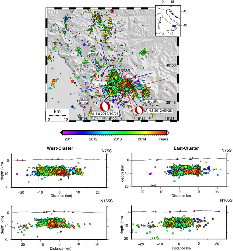
FIGURE 2. Map and sections of the 2011–2014 seismic sequence/swarm from ISIDe Working Group (2016), https://doi.org/10.13127/ISIDE. The size of the epicenters is proportional to the magnitude and star symbols depict events having M > 3.5. The epicenters are divided into two main clusters: Western and Eastern, enhanced on the map by blue and red ellipses. The cross-sections of the Eastern and Western clusters are plotted to the bottom.

FIGURE 3

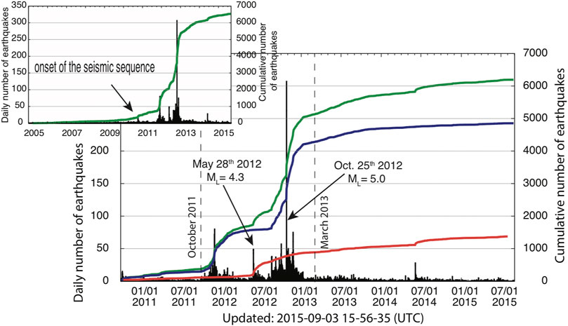
FIGURE 3. Temporal evolution of the swarm: black histogram defines the daily number of events, the green line is the cumulative number of events in the whole region, the blue line and the red line are the cumulative number of events for the western and eastern cluster, respectively. Only the blue line trend seems to follow a mainshock–aftershock behavior.

Preliminary hypocentral locations are concentrated at depths between 5 and 10 km during the entire swarm (data source: ISIDe working group 2016). The analysis of the Time Domain Moment Tensor (TDMT; http://cnt.rm.ingv.it/tdmt.html; Scognamiglio et al., 2009) recognized for the strongest events, two fault plane solutions consistent with normal faults striking ∼N25°W and dipping at about 45°. On the whole, focal mechanisms are coherent with a NE–SW extension observed in the area (Totaro et al., 2013).

The seismicity mainly occurred near the Mormanno village (western larger dashed ellipse in Figure 2). On May 28th, 2012, at about 5 km eastward of the first main cluster of seismicity a shallow M_L 4.3 event occurred (Figure 2). The seismic activity remained concentrated in this area (eastern smaller dashed ellipse in Figure 2) until early August. Thereafter, seismicity moved again westward to the Mormanno activated area, where several events with a magnitude larger than 3.0 preceded the strongest earthquake (M_L 5.0) that occurred on October 25th, 2012. The seismicity rate persisted high for some months, but magnitudes did not exceed M_L 3.7. At the beginning of 2013, the seismic activity started to decrease (inset in Figure 3), remaining relatively low until June 2014, when a magnitude M_L four earthquake occurred in the eastern cluster, giving rise to a sudden increase of the seismic rate in the surrounding area. The seismicity rate kept decreasing during 2015, although remaining above the background seismicity threshold (inset in Figure 3).

There is evidence that this seismic sequence behaves as a swarm more than as a mainshock-aftershock seismic sequence, in fact, this preliminary hypothesis is supported by a more accurate and detailed analysis performed by Passarelli et al. (2015); they found that 75% of earthquakes may be related to a transient forcing and only 25% could be interpreted as aftershocks, We show in Figure 3 the temporal evolution of the seismic sequence in term of seismicity rate to investigate different behaviors of the two clusters. The histograms of the daily number of events and the cumulative number of events for the whole area (green line in Figure 3) show an increase of the seismicity months before the mainshocks, with a seismic rate that increases and decreases at varying pace.

We also believe, when considered the two main clusters separately, that the events clustered inside the western area have swarm behavior (blue line in Figure 3); whilst the events occurred in the eastern region seem to follow a mainshock-aftershock trend (red line in Figure 3).

Temporary Seismic Network

During these four years of intense seismic activity, a group of temporary INGV seismic stations (INGV Seismological Data Center, 2006) and Deutsches Geo Forschungs Zentrum (GFZ) seismic stations and array (Passarelli et al., 2012) were installed, for the purpose of enhancing the earthquakes identification capability of the Italian National Seismic Network there in real-time (Figure 4, see also Govoni et al., 2013 for details) and to refine the accuracy of the locations using also off-line data. The temporary seismic network was composed of a variable number of seismic stations during the entire seismic sequence, from eight stations in late 2011 to about 20 stations in late 2012, in order to refine the hypocentral locations of small-magnitude earthquakes and ensure a lower magnitude detection threshold of the network (see also De Gori et al., 2014, for the timing of stations deployment). In May 2015 the temporary network deployed in the Pollino region was removed keeping only two stations to maintain a lower magnitude detection threshold in the area with respect to the regional standard.

FIGURE 4

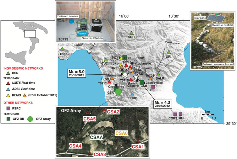
FIGURE 4. Map of temporary and permanent seismic networks deployed in the area during the seismic activity. In the upper insets an example of installation is reported; in the lower panel is shown the GFZ seismic array configuration. In the map, the two main-shocks are also reported as white stars.

Refined Earthquakes Location

The analysis of the seismic sequence greatly benefited from data provided by the temporary seismic stations installed soon after the sequence started (Figure 4), many of which contributed to the real-time monitoring (Govoni et al., 2013). Earthquakes were originally located by analysts on seismic surveillance duty with the HYPOINVERSE-2000 code (Klein, 2002) using a 1D velocity model with two layers at 0–11 km (Vp = 5.0 km/s) and 11–38 km (Vp = 6.5 km/s) depth over a half-space at depth >38 km with Vp = 8.0 km/s. These locations (Figure 2), available in real time on the ISIDe website, were used as the initial dataset.

For this study, we carefully reprocessed the earthquakes reading P- and S-phases arrivals on the three-component digital recordings at local stations from October 2011 to March 2013. As the first step, we located all the earthquakes using the program Hypoellipse (Lahr, 1989) and a starting Vp model taken from Chiarabba et al., 2005, adopted for the whole Italian region.

The average Vp/Vs in the crustal volume where seismicity developed has been estimated through the modified Wadati method (Chatelain, 1978). Since seismicity mainly occurs at depths of 5–10 km, most of the observations consist of up-going ray-paths, thus the retrieved Vp/Vs (1.81, see Figure 5A) is strongly representative of the focal volume.

FIGURE 5

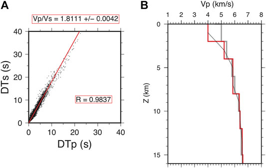
FIGURE 5. (A)Wadati (1933) diagram computed on all the earthquakes with up-going ray-paths to the stations. For each event, DTp and DTs are the differences between P- and S-phase arrival times, respectively, at couples of stations. The Vp/Vs value is the slope of the straight red line, while R is the correlation coefficient of the linear regression (B) Starting (dark gray) and final (red) P-wave 1-D velocity model computed using the VELEST code (Kissling et al., 1994).

Locations With Minimum 1D Velocity Model

In order to improve earthquake locations, we computed an ad hoc 1D velocity model by applying the inversion scheme introduced by Kissling et al. (1994) and implemented in the code VELEST. To obtain a stable 1D reference model, we selected a subset of events that meet the following selection criteria: rms <0.5, azimuthal gap <200°, location errors within 2 km, and at least seven P- and 3 S-wave readings.

We then inverted P- and S-wave arrival times, from a subset of 808 selected earthquakes, to simultaneously compute hypocenter solutions and the minimum 1D velocity model parameterized by horizontal layers with Vp values varying with depth. The damping parameter was chosen by running different inversions as the best trade-off between data variance reduction and model complexity. The optimum model (Figure 5B) was achieved after 10 iterations, obtaining a final rms of 0.12s with a variance reduction of 48%.

Below a thin layer of sediments cover, with a thickness of 2 km and Vp of 4 km/s, the P-wave velocity (Figure 5B) displays values characteristic for consolidated sedimentary rocks like Mesozoic evaporites and carbonates, in agreement with the velocity values found by Improta et al. (2017), in an adjacent area.

The retrieved relatively high Vp/Vs values (1.8) is often observed in Mesozoic carbonate rocks of the Apennines and can be related to fracturing and fluid saturation (e.g., Improta et al., 2014).

Finally, we use this minimum 1D model to relocate the whole set of earthquakes through the Hypoellipse code (Lahr, 1989). We obtain a final set of 2,323 well located earthquakes; the performance of the adopted approach, in terms of rms and location errors can be evaluated in Figure 6.

FIGURE 6

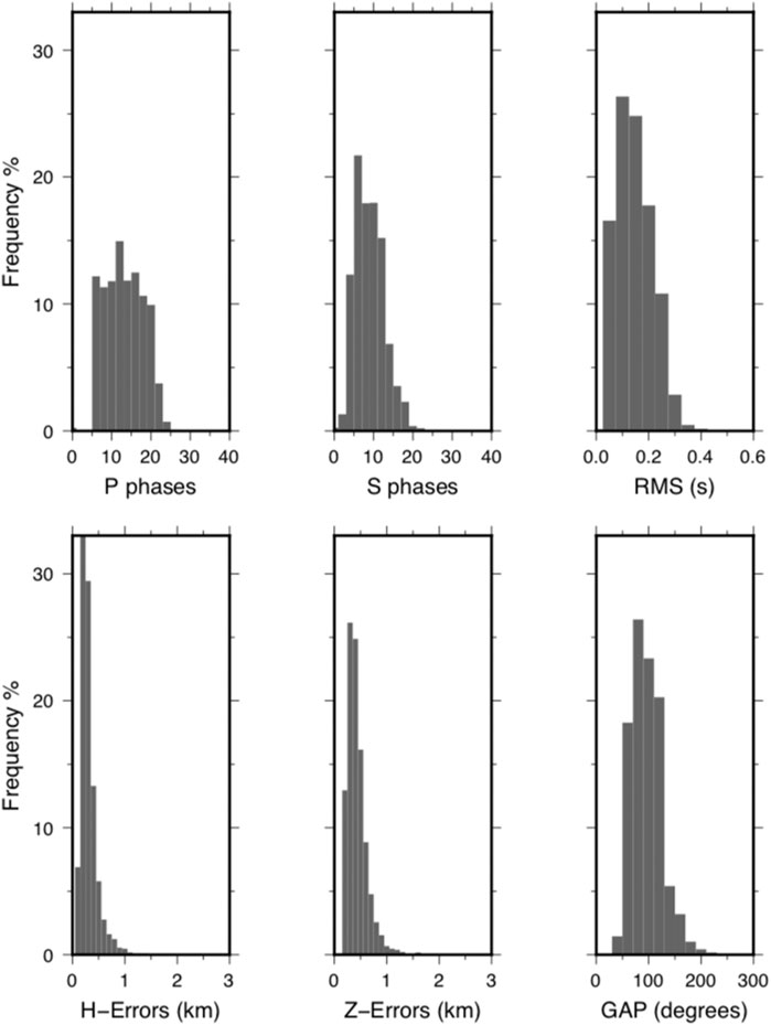
FIGURE 6. Histograms summarizing the main outputs of the localization procedure, in terms of frequency of observations for each of the following parameters (from top left to bottom right): number of observations for P phases; number of observations for S phases; residual rms (s); horizontal location errors (km); vertical location errors (km); azimuthal gap between stations (°).

Results of the analysis described above are shown in Figure 7, where map and cross section views of the seismic sequence are provided. The relocated earthquake catalog represents a sensible improvement with respect to that shown in Figure 2 in terms of geometrical definition of the activated fault system, whose characteristics are here recognizable.

FIGURE 7

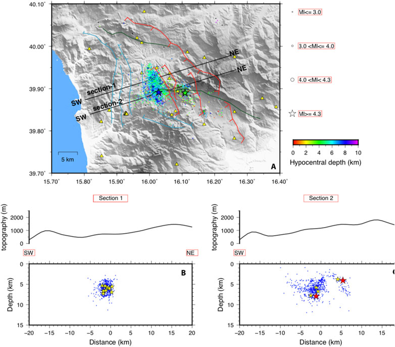
FIGURE 7. Map and cross sections view of the earthquakes relocated using the minimum 1-D model (A) The top image shows a map of the epicenters, where earthquakes are sized by magnitude according to the symbols on the right of the map and color-coded by hypocentral depth according to the scale on bottom. The M_L 5.0 and M_L 4.3 mainshocks are represented by stars. Yellow triangles are permanent and temporary seismic stations. Black lines are the traces of the vertical cross-sections. See Figure 1A for major structures description. Two main clusters are recognized: the first one to the West and the other on the East, which include the M_L 5.0 and M_L 4.3 events, respectively (B, C) On the cross sections -1, and -2, we project all the events located within 1 km from the vertical plane. (B) The hypocenters, in section-1, in the northern part of the sequence, depict a ball-shaped seismogenic volume. (C) The hypocenters, in section-2, on the south, seem to delineate three seismogenic faults. On both the cross sections, the M_L 5.0 and M_L 4.3 mainshocks are represented by the red stars while the yellow stars identify epicenters with a magnitude larger than 3.0.

The analyzed earthquakes describe two main areas of seismicity: Western and Eastern clusters; in the first one, the M_L 5.0 is located instead in the second one the M_L 4.3 occurred. The cross-sections well delineate two different behaviors: in the northern cross-section (Figure 7B) the hypocenters define a ball-shaped volume without imaging any planar lineament. The distribution of the M_L >3.0 best-recorded events in the area (yellow stars in Figure 7B), also agrees with more diffuse seismicity rather than depicting a planar one.

On the contrary, in the southern cross-section (Figure 7C), hypocenters define at least three dipping fault planes. Those planes include the one potentially responsible for the M_L 5.0 event, which was imaged by the seismicity hypocenters also before the occurrence of such mainshock. This plane has been reconstructed with a similar geometry also by other recent studies (Brozzetti et al., 2017; Napolitano et al., 2021). But with respect to these latter works, thanks to the ∼2,300 events analyzed and re-located, we were also able to depict an antithetic E-dipping fault plane located to the West of the main fault plane, and another NE-dipping, on the East, related to the M_L 4.3 event, possibly the source of this second mainshock.

Relative Locations With hypoDD

To further improve locations, we applied the double-difference (DD) relocation algorithm using the hypoDD code (Waldhauser and Ellsworth, 2000; Waldhauser, 2001). The algorithm minimizes the residuals between observed and calculated travel-time differences for pairs of earthquakes at common stations by iteratively adjusting the difference between the hypocenters. This condition holds if the hypocentral distance between earthquakes is small compared to the source receiver separation.

We used P and S wave arrival times picked from three component seismograms, the starting locations derived above and the minimum 1D velocity model already described. Double-differences are generated to link each event to several neighbors, so that all the events are connected and the adjustment to hypocenter parameters is simultaneously determined. In our case, all the selected events are strongly linked to the others forming one main cluster. We performed 10 iterations optimizing the damping parameter to obtain good conditioning and convergence of the solution. The iterations were grouped into three sets for better control of the inversion procedure and to achieve a consistent convergence. The final adjustments are in the order of meters.

The DD locations show a seismicity distribution similar to that obtained with the minimum 1D model, but emphasizes some aspects of the geometry like the opposite dipping of the two main faults (Figure 8). The northern part of the main cluster still does not present a clear planar geometry.

FIGURE 8

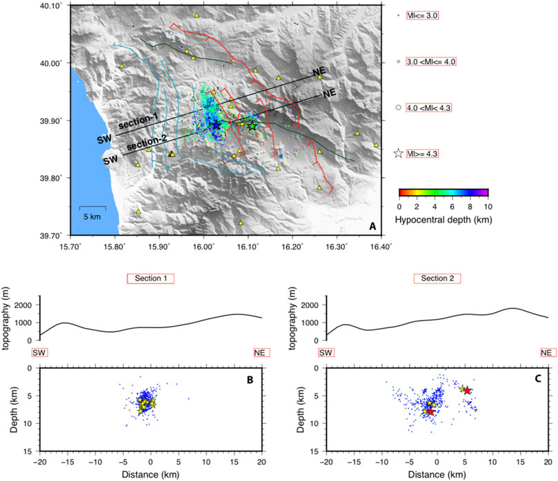
FIGURE 8. Map and cross sections view of the earthquakes relocated using the hypoDD location. Layouts and symbols are the same as in Figure 7.

Shear-Wave Splitting

From ∼6,000 events recorded at temporary (T07*) and permanent stations deployed in during the seismic sequence, we analyzed 22,623 event-station pairs looking for crustal anisotropy to evaluate the shear wave splitting parameters: fast direction polarization (φ) and delay time (δt). Seismicity used in the anisotropic analysis is mainly concentrated under Mormanno village between 5 and 10 km depth, with magnitudes ranging from 0.2 to 3.0. To avoid complications on the S-wave arrival, due to the P-wave coda of a strong events that could make difficult the splitting analysis, we decided to discard events with a magnitude greater than 3.0. We used Anisomat+ (Piccinini et al., 2013) a set of MatLab scripts able to retrieve automatically φ and δt from the seismic recording of local earthquakes. We tuned this code by using a standard configuration for local earthquakes, already tested in other studies, such as in Pastori et al. (2019) for the Amatrice–Visso–Norcia seismic sequence and in Baccheschi et al. (2016) for the L'Aquila earthquake, applying the following values: (1) Corner frequencies of cf1 = 1 Hz and cf2 = 12 Hz of the four poles 2 pass Butterworth filter; (2) PRE variable set on 0.15 s time before the S-picking in which the analysis window starts; (3) DUR variable, representing the time after the S-picking, is computed using the formula DUR = C 1/cf2 where C is a coefficient, in this case set on 2.5 to ensure including at least a complete filtered shear wave cycle; (4) the total duration of the analyzed signal is 0.35 s (PRE + DUR) and encompass the S-wave arrival.

To ensure that the observed shear wave energy pertains only to the horizontal plane, the code performs a number of tests. In detail, the code evaluates i) the S-to-P ratio, the ratio between the amplitude of the horizontal components sum (RMSs) and the amplitude of the vertical component (RMSp) computed on the analysis window as RMSs/RMSp and it is set to be greater than four; ii) the geometrical incidence angle computed as ic = sin-1(Vs/Vp) is set to be lower than 45° (Booth and Crampin, 1985), where Vs and Vp are the velocities of S and P waves, respectively.

Following Bowman and Ando (1987) Anisomat + calculate the cross-correlation between the two horizontal components. This allows measuring the similarity of the pulse shape between the S-waves and their delay time (δt). These two time series in fact have similar shapes, mutually orthogonal oscillation directions, and travel with different velocities.

Horizontal components of the ground motion are then rotated (with steps of 1° from 0 to 180) and for each step, the cross-correlation function is stored. Finally, a two-dimensional matrix is obtained and after a grid search, the code estimates the couple of lag time and rotation angle which maximizes the cross-correlation coefficient.

These two quantities represent the delay time between the slow and fast shear wave (δt) and the polarization azimuth (φ) of the incoming fast shear wave.

Associated errors are defined by a criterion that reflects the shape of the cross-correlation matrix and how rapidly the matrix grows around the observed maximum value. In practice, the goodness of the estimation is related to the difference in delay time and in degrees between the cross-correlation maximum and 95% of the parameter values themselves. The mean errors for fast directions and delay times are 14.7° and 0.008 s, respectively (see Table 1 for mean values at each station). At the end the code returns an ASCII output file composed by 21 fields described in the Supplementary Material. For further details, the reader should refer to Piccinini et al., 2013.

TABLE 1

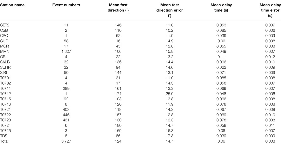
TABLE 1. Averaged anisotropic results and their associated errors obtained at each used station.

Seismicity used in the anisotropic analysis is mainly concentrated under Mormanno village between 5 and 10 km depth, with magnitudes ranging from 0.2 to 3.0. To avoid complications on the S-wave arrival, due to the P-wave coda of a strong event that could make difficult the splitting analysis, we decided to discard events with a magnitude greater than 3.0.

After the Anisomat + analysis and its quality controls, in order to discuss a high-quality anisotropic dataset, we admitted only those results with a cross-correlation coefficient CC ≥ 0.75, which allowed us to obtain a total of 3,727 fast single measurements (δt > 0.02 s) and 2,040 null results (δt ≤ 0.02 s). A measure is defined null when the S wave does not show splitting; this happens, in an anisotropic medium, when the initial S-wave polarization is coincident to the slow or the fast axis, and furthermore, nulls do not constrain the delay time.

We present the fast and null directions as interpolated values on a regular grid-box which nodes are 2-km spaced (see Supplementary Figure S1 for details) evaluated with the Tomography Estimation of Shear wave splitting and Spatial Averaging (TESSA) program (Johnson et al., 2011). In each block, the rose diagram of fast values and the associate mean fast direction are displayed, providing i) the standard deviation is <30°, ii) the standard error is <10°, and iii) at least 10 rays pass through the grid-box. Furthermore, TESSA weights the data according to the fast errors estimated by means of Anisomat+ and to the weighting regime selected, in this case, we chose a 1/d regime, where d is the length in km between the grid-box and the station. The insets of Figure 9, the orange and green rose diagrams are frequency plots representing splitting fast and null measurements, respectively, for the whole area. Prevalent NW-SE fast directions are observed: the average fast direction is N124° (see Table 1 for mean values at each station) while the null directions show two main peaks one strikes N127° (considered as the fast direction) and the other roughly orthogonal to it (considered as the slow direction).

FIGURE 9

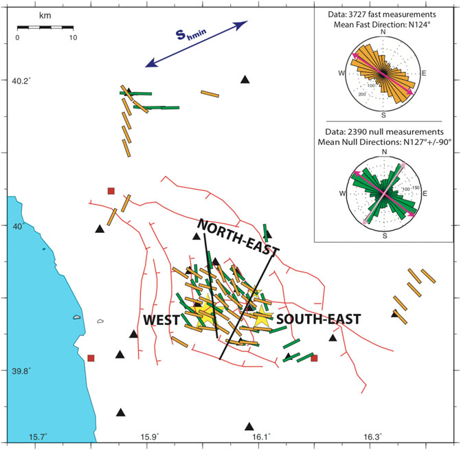
FIGURE 9. Map of the spatial average for 3,727 fast (orange bars) and 2040 null (green bars) measurements. Three sectors are recognized: West) even if a WNW–ESE mean direction is observed, fast and null orientations are variables and not coincident; North-East) a NNW–SSE mean direction is visible, fast and null orientations are stables and coherent; South-East) a trend from NW–SE to E–W mean direction is delineated from both fast and nulls measurements. The upper right insets show the total rose diagrams for both fast and null measurements.

In the crustal volume sampled by S-waves, the different mean fast directions observed lead us to suppose the presence of intense and complex anisotropic anomalies. The prevalent φ is both parallel to the major fault structures and consistent with the local stress field being parallel to the NW–SE S_Hmax, so the ambiguity on the probable crustal anisotropic source is not solved: structural anisotropy or aligned microfractures opened by the active stress field?

Fast orientations delineate three main areas North-East, West and South-East: 1) NNW–SSE mean direction (stable and coherent for fast and null measurements); 2) WNW-ESE mean direction (variable and not coincident for fast and null measurements) and 3) from NW-SE to E-W mean direction (stable and coherent for fast and null measurements), respectively.

In the north area of the activated fault system, the relocated hypocenters define a diffuse ball-shaped volume of seismicity instead of fault planes. This behavior could have influenced the anisotropic parameters, in fact, the strong variability of fast directions, noticed in the western area, can indicate the absence of dominant structures and the existence of a complex diffusivity system where fluids can flow. Instead, in the eastern part where the hypocenters delineate a main SW-dipping fault plane with an antithetic plane to the west and another dipping to NE on the east side (Figures 7C, 8C), we observed stable and coherent φ with respect to the major structures, in this case, we can assume that anisotropy is structurally controlled as predicted by Zinke and Zoback (2000) structure-related model.

Delay time singular values oscillate between 0.024 up to 0.248 s (Figure 10A) with a total average value of 0.06 s (see Table 1 for mean values at each station). These values agree with those found in other regions of Italy along the Apennine (Margheriti et al., 2006; Piccinini et al., 2006; Pastori et al., 2009; 2019), or in the crust of other regions in the world, as on the Karadere–Düzce fault (Peng and Ben-Zion, 2004). We will interpret the results in terms of delay time normalized for the hypocentral distance (δtn) because we suppose that the anisotropy measured at the station is just the sum of the anisotropic structures crossed by the seismic ray (e.g., Crampin, 1991; Zhang et al., 2007).

FIGURE 10

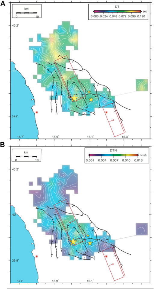
FIGURE 10. Geographical distribution of (A) delay time and (B) normalized delay time values interpolated on a 2 km spaced grid, by means a nearest neighbor algorithm.

Normalized delay time values are represented in Figure 10B as the geographical distribution of interpolated single measurements on a 2-km spaced grid, similar to that used for the fast measurements averaging. The higher culmination of δtn (from 0.007 to 0.01 km/s) is visible in the Northeast sector that represents the hangingwall of the fault that generated the M 5.0 event. This value allows us to confirm that the principal source of crustal anisotropy, in this area, is represented by the structural control, as already seen by the φ pattern.

The lower values of δtn (from 0.003 to ∼0.005 s/km) are visible in the external west and southeast areas. These values allow us to suppose the presence of a complex diffusivity fluid system where fluids can migrate along a relatively high-permeability hydraulic path but cannot be gathered. The existence of this network of fractures and/or porous fluid-filled is also invoked, i. e, by Della Vedova et al. (2001) to interpret the unusual low geothermal gradient of the region, by Barberi et al. (2004) and Totaro et al. (2014) to explain an high Vp/Vs value observed in the shallowest crust and by Napolitano et al. (2020) to justify the scatter and absorption anomalies.

Discussion

The Pollino gap area is located at the edge of the southern Apennines where a broad strike-slip shear zone separates two lithospheric blocks (the Apennines and the Calabrian arc) with different evolution in the Plio-Pleistocene (Spina et al., 2009; Orecchio et al., 2015; Palano et al., 2017). This lithospheric discontinuity favored the retreat of the ionian slab during the lower Pleistocene and consists of a set of N120-trending faults, which comprises the Pollino fault and the Amendolara fault in the ionian off-shore (Ferranti et al., 2014).

In Late Pliocene-Quaternary the ancient thrust structures are crosscutting by extensional faults that forming intermountain basins along the Apennines axis (Ferranti et al., 2017), as well as the Mercure and the Crati basins respectively to the North and South of the Pollino fault.

Common tectonic models are based on the continuity of deformation between the southern Apennines and Calabrian arc (i.e., Valensise and Pantosti, 2001); lateral heterogeneities across the Pollino mountain range instead suggest that the strike-slip shear zone permits a kinematic decoupling between the extending Apennines and that retreating Calabrian block (Chiarabba et al., 2016), as also signaled by the imprint of toroidal flow at the ionian slab edge on GPS data (Palano et al., 2017).

The Quaternary normal active fault systems segmented by the tectonic structures inherited from the past and the complex interaction between the activated fault planes evidenced by the refined 1D and DD relocations can be considered as the cause of the great variability defined by the anisotropic pattern.

Recent studies tried to model the geometry of the activated fault system in this area. Napolitano et al. (2021) used a smaller portion of events (422 in 27 clusters) with respect to our dataset (∼2,300 events). Their locations were concentrated mainly on the western cluster and depicted a structure, having a similar geometry to the one that we consider to be probably responsible for the M_L 5.0. On the contrary, they did not identify the antithetic fault, that we assume likely causing the M_L 4.3, because their data did not sample the eastern cluster.

Brozzetti et al. (2017) used both seismological and geological data to infer the geometry of activated faults. Their solutions agree with the geometry of the M_L 5.0 reconstructed by our data, on the other hand, to define the fault causative of the M_L 4.3, their locations showed an almost vertical alignment of earthquakes and considering the geological surface expressions they preferred a fault dip to the NE.

In our study, we compare refined 1D and DD locations and anisotropic results to better constrain the geometries of the activated fault system. The S-waves fast polarizations show a general rotation from roughly WNW–ESE (sub-parallel to CaF) to NNW–SSE (sub-parallel to the ROCS active extensional systems) to WNW–ESE (sub-parallel to the Pollino line) (orange bars in Figure 11A). Such orientations are also observed in null results, except for the Western area (green bars in Figure 11A); as previously explained we observe a null direction if the initial S-wave polarization is coincident to the source structures of the anisotropy. After these considerations, we can affirm that for the western sector, fast direction polarizations are probably more related to aligned microfractures opened by the active stress field, while nulls reflect major structure orientations confirming a structural control of anisotropy.

FIGURE 11

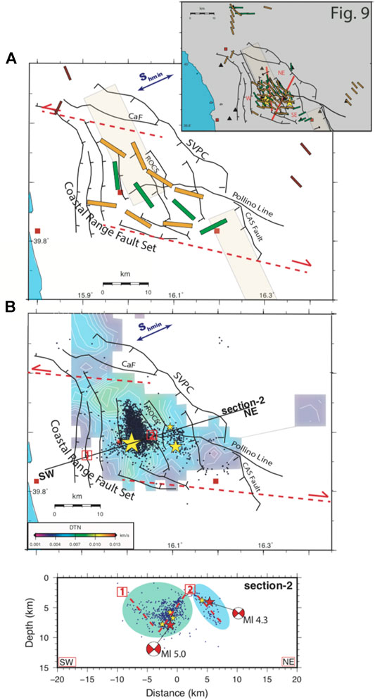
FIGURE 11. (A) Sketch map of the identified three sectors with similar mean fast and null directions. In general, a rotation from roughly WNW–ESE to NNW–SSE and WNW–ESE is observed. These orientations are related to major active faults, such as CaF, ROCS, and Pollino line, respectively, except for the West sector where fast and null directions are not in agreement. (B) Map of interpolated values of δtn and the superimposed 1D relocated seismicity. (C) Southern cross-section of 1D accurate location; green and blue shadow are referred to as δtn values, and dashed lines define the activated fault systems. In (B)–(C), 1 and two represent the top points of the probable fault planes projected in map. 1 falls into the CRFS area while two falls into the intersection between the ROCS area and the westernmost part of the Pollino line. In (A)–(B), red dashed lines with arrows represent the regional scale strike-slip episodes related to geodynamic processes, yellow stars identify the strongest events, and the main fault systems are also reported.

All these orientations well-delineate the regional scale structural complexities, such as the strike-slip episodes related to geodynamic processes and those at the small-scale represented by the local stress variations.

In general, the interaction between the irregular geometries of the fault systems could favor multisegment ruptures and/or the reactivation of inherited structures with the inversion of the kinematics due to the present stress regime. These segments take part in the generation of a complex diffusivity system where fluids can be channelized and carried toward heavily fractured rock volume where in some cases they can be gathered.

Overall, we found in the western sector, the volume where most of the seismicity occurs, a higher value of δtn. This crustal volume represents, under a structural point of view, the hangingwall of the main fault where the M 5 is supposed to be enucleated. Similarly, the 1D and DD accurate relocations depict a SW-dipping main fault plane but also an antithetic plane to the west. This area can be imaged as an ancient positive flower structure reactivated in the current extensional regime, as also considered by Totaro et al. (2015) to explained their focal mechanism solutions and high-precision locations using the DD method in the Mercure Basin.

The main faults, that border the flower structure, could play the role of a preferential pathway in which fluids are channelized and accumulated on the top of the heavily fractured rock volume and laterally confined by these structures (Figures 11B,C).

Instead, in the southeast sector, the 1D and DD relocation possibly represents a NE-dipping plane where the fewest seismicity occurs. In this area, the anisotropic pattern of fast directions recognizes a dominant WNW–WSW trend and lower value of δtn. These findings suggest that fluids migrate preferentially along hydraulic pathways having a high percentage of permeability, such as the hypothesized secondary fault, up to the free surface not allowing a constant pervading the crustal volume by fluids.

Seismogenesis

In the hangingwall of the activated fault systems (western sector), our anisotropic evidence and the excess rate of seismicity during the sequence are indicative of countless fluid-saturated cracks. Napolitano et al. (2020) through a study based on seismic scatter and absorption confirmed the presence of a highly fluid-filled micro-fractured seismogenic volume around the main activated structures during the swarm. Passarelli et al. (2015) established that the temporal and spatial behavior of seismicity in the western sector follows prevalently a swarm-like consistent with a transient, external forcing. Even Cheloni et al. (2017) evidenced a transient slip, around the mainshock, approximately 4 months before and gone on about one year.

Transient slip associated with a high percentage of fluid-filled fractures could have reduced the effective normal stress facilitating fault slip, partially inhibiting the development of large rupture (Cheloni et al., 2017; Yoshida and Hasegawa, 2018), increasing the rate of seismicity but limiting the maximum magnitude of events.

Furthermore, also lithology might affect the permanence of fluids, in fact, the carbonate rocks forming the hangingwall have an important function in both preserving and hosting the micro-fracture system responsible for the observed anisotropic pattern. This permanent presence of fluid could reduce the long-term fault strength, promoting aseismic fault slip and causing important weakening along the existing fault planes. In this contest, looking at the structures obtained by the 1D and DD relocations we can suggest the reactivation of an ancient positive flower structure in the actual stress regime.

We, therefore, explain the space-time-magnitude pattern of the seismic sequence, and the excess rate of seismicity, as governed by the preservation of the filled-fluid micro-fracture network in the seismogenic volume that followed transient slip.

Constraints to Hazard

Persistent swarms in the Pollino seismic gap area created repeated concerns in public and seismic risk stakeholders, for uncertainties on possible forecasting scenarios. Most of the concerns derived from the perception that the area was seismically silent for a long time and possibly prone to a large event. The analysis of the 2011–2014 swarm yields therefore precious information that might help to constrain hazard models.

The seismic gap idea, first expressed by Omori (1908), was motivated by the lack of large earthquakes since at least 10 Kyr (Rovida et al., 2016). In the continuous extensional fault system model (Valensise and Pantosti, 2001), a 60 km long gap encloses the Pollino mountain range and partially the upper Crati valley. The faults studied by paleo-seismological trenches in the southern border of the Pollino area evidenced large slip earthquakes older than 1 Kyr (Galli et al., 2008; Cinti et al., 2002; Michetti et al., 1997), reinforcing the idea that large earthquakes are expectable.

The absence of large earthquakes in the historical catalog has been associated with a combination of low strain rate and mixed seismic/aseismic strain release that could increase the recurrence time of large magnitude events (Cheloni et al., 2017).

Under these circumstances, the persistence of a pervasive fluid system network in the pop-up structure accounted for increasing the stability of the faults, partially inhibiting the generation of large earthquakes. In any case, the reactivation of pre-existent thrusts and back-thrusts of the pop-up would promote the segmentation of the seismic gap in fragments with a maximum length of 10–12 km.

Although shear wave splitting analysis does not measure directly the activity of a fault, our results might help us to delineate the seismotectonic settings of the Pollino region.

In the western sector, where the highly fractured rock and the excess rate of seismicity are observed, we can suppose a reduction of shear-strength along CRFS and ROCS faults (Figures 11B,C), probably representing the boundaries of the flower structure. This reduction in turn can generate earthquakes also for a low level of stress accumulation.

In the eastern sector, instead, the lower values of δtn and fewer seismicity rates are concentrated; this area coincides with the upward continuation of the surface expression of CAS (Cinti et al., 2015). The absence of a strong pervasive fluid system network that reduces the effective normal stress facilitating fault slip, around the intersection between CAS fault might suggest that this eastern segment could be more prone to an unstable deformation and a large rupture.

Differences in Crustal Response to Slab Tearing Between Apennines and Calabria

Comparing Figures 7B,C, 8B,C strikingly illustrates the different behavior in the release of seismic energy between the Northern half and the Southern half of the study area. While a more standard seismicity clustered along defined planes is present in the Southern half (Figures 7C, 8C), diffuse seismicity is found in the North (Figures 7B, 8B). Those two phenomena have been observed worldwide, but rarely in such close proximity. We speculate that such rapid spatial change in crustal behavior is caused by a different response of the Southern Apennines and the Calabrian block to the tearing of the ionian slab. Slab tearing is likely to generate diffuse deformation in the overriding plate (i.e., Maesano et al., 2020; Chiarabba and Palano, 2017; Gutscher et al., 2016). The Apennines slab has been torn in several places (Rosenbaum et al., 2008) and the tearing process has shown to affect the entire crustal volume (Bianchi et al., 2016). Such “crustal response” is likely to interest a wide area rather than a focalized rock volume on top of the tear fault (Rosenbaum et al., 2008), depending on the local rheological properties of the crust (Boncio et al., 2007; Polonia et al., 2011). Here the tearing of the ionian slab, revealed at depth by passive seismic (Rosenbaum et al., 2008; Orecchio et al., 2015), probably interested in different ways the juxtaposed two crustal domains, focusing a higher level of deformation on the Southern Apennines side, and, thus, weakening the entire crustal volume. This interpretation is supported by the distribution of earthquakes in a diffuse area (NW of Mormanno) indicating the inability of cumulating stress on relevant tectonic structures (i.e., km-scale planar faults) and corroborated by the misoriented fast polarization directions with respect to the major structures, given by the complex fluid-filled fracture network. Opposite observations in the Southern portion (planar faults, where main M_L 5.0 and M_L 4.3 events occurred) where fast directions reflect the strike of the major structures testifying to the different behavior of the crustal response to slab tearing, on the two sides of the boundary between Apennines and Calabria.

Conclusion

The seismic swarms occurred within the gap area, along the Pollino shear zone. Relocated earthquakes reveal that seismicity developed on two main NNW-trending and opposite dipping clusters with primary events being the M_L 4.3 and the M_L 5.0 on 28th May and 25th October 2012, respectively.

The geometry drawn by the refined 1D and DD locations delineates the activated fault system having the following characteristics: a) it is composed at least of three fault segments with a length <10 km; b) it is located in the shallower 10 km of the crust; c) it is oriented roughly NW-SE. The dip of the main fault segment, where most of the seismicity occurs such as the M_L 5.0 earthquake, is toward SW while, the two other minor segment faults dip toward NE. Although with a lower resolution also Totaro et al. (2014) pointed out a similar geometry of the main fault segment.

According to the data reported in DISS database, we could place the activated fault system between the two major seismogenic sources present in the area: the Rimendiello–Mormanno Mercure Basin fault system (RM-MB) and the Castrovillari Fault (CV). The geometry of the RM-MB, constrained by geological data, is about comparable with the trend of the recent seismicity, but its dip is to the NE. Instead, CV source has a similar orientation (N20W) and a western dip, as reported by the analyzed seismicity, but its northern border match to the southernmost epicentres. Finally, our results in terms of fault orientations delineated at depth by 1D and DD refined locations could be connected to the mapped fault systems reported by Brozzetti et al. (2017).

The reactivation of an ancient positive flower structure in the actual stress regime is supported by the fast direction polarization rotation from NNW–SSE in the middle of the extensional basin toward WNW–ESE in the area where the Pollino fault is supposed to be. As imaged by location earthquakes this structure is composed of a set of thrust and back-thrust strikes mainly NW–SE.

The interaction at a depth between these faults could generate a pathway for fluids and in certain conditions, i.e. in the presence of a structural barrier, reach the overpressure status. As observed from anisotropic results, the presence and mobility of channelized fluids in the crust promote multisegment ruptures and/or the reactivation of inherited structures only if favorable oriented with the present-day stress regime.

Back thrust reactivation contributes to the segmentation of the 60 km long seismic gap in fragments with a maximum length of 10–12 km. In this vision, the subdivision could partially restrict the generation of large earthquakes in this area.

Data Availability Statement

The data of used stations are from the Italian National Seismic Network (doi.org/10.13127/SD/X0FXnH7QfY). The waveform data of earthquakes used are available at EIDA database (European Integrated Data Archive http://eida.rm.ingv. it/).

Author Contributions

MP wrote the manuscript, analyzed the data and evaluated the anisotropic parameters; LM coordinated the working group; PDG, AM and DL made picking analysis and 1D locations; AG installed the temporary stations in the field, made data available and helped in the discussions; FL, NA, DP and CC made picking analysis and discussed the results; MM coordinated the fieldwork and made picking analysis; PDL made picking analysis and evaluated anisotropic parameters; RDG, MA and AN made picking analysis; LP discussed the results.

Funding

This study has benefited from funding provided by the Italian Presidenza del Consiglio dei Ministri –Dipartimento della Protezione Civile (DPC). This paper does not necessarily represent DPC official opinion and policies.

Conflict of Interest

The authors declare that the research was conducted in the absence of any commercial or financial relationships that could be construed as a potential conflict of interest.

Acknowledgments

We would like to thank all operators who installed and serviced the temporary seismic stations managed by INGV. We would like to follow up by thanking all the INGV staff on shifts in the surveillance room in Rome for their work and the Bollettino Sismico Italiano working group (http://terremoti.ingv.it/bsi) for making available the files of the manually revised P- and S-phase pickings. We are grateful for the comments and suggestions of the Guest Associated Editor Jorge Gaspar-Escribano, Luca De Siena, and the reviewer, which helped us to improve the final version of the manuscript.

Supplementary Material

The Supplementary Material for this article can be found online at: https://www.frontiersin.org/articles/10.3389/feart.2021.618293/full#supplementary-material.

References

Baccheschi, P., Pastori, M., Margheriti, L., and Piccinini, D. (2016). Shear wave splitting of the 2009 L'Aquila seismic sequence: Fluid satu- rated microcracks and crustal fractures in the Abruzzi region (central Apennines, Italy). Geophys. J. Int. 204 (3), 1531–1549. doi:10.1093/gji/ggv536

CrossRef Full Text | Google Scholar

Barberi, G., Cosentino, M. T., Gervasi, A., Guerra, I., Neri, G., and Orecchio, B. (2004). Crustal seismic tomography in the Calabrian Arc region, south Italy. Phys. Earth Planet. Inter. 147 (4), 297–314. doi:10.1016/j.pepi.2004.04.005

CrossRef Full Text | Google Scholar

Bianchi, I., Lucente, F. P., Di Bona, M., Govoni, A., and Piana Agostinetti, N. (2016). Crustal structure and deformation across a mature slab tear zone: the case of southern Tyrrhenian subduction (Italy). Geophys. Res. Lett. 43, 12380–12388. doi:10.1002/2016GL070978

CrossRef Full Text | Google Scholar

Boncio, P., Mancini, T., Lavecchia, G., and Selvaggi, G. (2007). Seismotectonics of strike–slip earthquakes within the deep crust of southern Italy: geometry, kinematics, stress field and crustal rheology of the Potenza 1990–1991 seismic sequences (Mmax 5.7). Tectonophysics 445 (3–4). 281–300. doi:10.1016/j.tecto.2007.08.016

CrossRef Full Text | Google Scholar

Booth, D. C., and Crampin, S. (1985). Shear-wave polarizations on a curved wavefront at anisotropic free surface. Geophys. J. Roy. Astron. Soc. 83, 31–45.

CrossRef Full Text | Google Scholar

Bowman, J. R., and Ando, M. (1987). Shear-wave splitting in the upper-mantle wedge above the Tonga subduction zone. Geophys. J. Int. 88, 25–41. doi:10.1111/j.1365-246x.1987.tb01367.x

CrossRef Full Text | Google Scholar

Brozzetti, F., Cirillo, D., de Nardis, R., Cardinali, M., Lavecchia, G., Orecchio, B., et al. (2017). Newly identified active faults in the Pollino seismic gap, southern Italy, and their seismotectonic significance. J. Struct. Geol. 94, 13–31. doi:10.1016/j.jsg.2016.10.005

CrossRef Full Text | Google Scholar

Brozzetti, F., Lavecchia, MilanaG., G., Milana, G. G., and Cardinali, M. (2009). Analysis of the 9 september 1998 Mw 5.6 mercure earthquake sequence (southern Apennines, Italy): a multidisciplinary approach. Tectonophysics 476, 210–225. doi:10.1016/j.tecto.2008.12.007

CrossRef Full Text | Google Scholar

Brozzetti, F. (2011). The Campania-Lucania Extensional Fault System, southern Italy: a suggestion for a uniform model of active extension in the Italian Apennines. Tectonics 30, 114. doi:10.1029/2010TC002794

CrossRef Full Text | Google Scholar

Chatelain, J. L. (1978). Etude fine de la sismicité en zone de collision continentale au moyen d'un réseau de stations portables: la région Hindu-Kush Pamir. Thèse de doctorat de 3ème cycle Université scientifique et médicale de Grenoble. Berlin: Springer, 219.

Cheloni, D., D'Agostino, N., Selvaggi, G., Avallone, A., Fornaro, G., Giuliani, R., et al. (2017). Aseismic transient during the 2010-2014 seismic swarm: evidence for longer recurrence of M ≥ 6.5 earthquakes in the Pollino gap (Southern Italy)? Sci. Rep. 7 (576), 576. doi:10.1038/s41598-017-00649-z

PubMed Abstract | CrossRef Full Text | Google Scholar

Chiarabba, C., Agostinetti, N. P., and Bianchi, I. (2016). Lithospheric fault and kinematic decoupling of the Apennines system across the Pollino range. Geophys. Res. Lett. 43, 3201–3207. doi:10.1002/2015GL067610

CrossRef Full Text | Google Scholar

Chiarabba, C., De Gori, P., and Speranza, F. (2008). The southern Tyrrhenian subduction zone: deep geometry, magmatism and PlioPleistocene evolution. Earth Planet. Sci. Lett. 268 (1–2), 408–423. doi:10.1016/j.epsl.2008.01.036

CrossRef Full Text | Google Scholar

Chiarabba, C., Jovane, L., and DiStefano, R. (2005). A new view of Italian seismicity using 20 years of instrumental recordings. Tectonophysics 395, 251–268. doi:10.1016/j.tecto.2004.09.013

CrossRef Full Text | Google Scholar

Chiarabba, C., and Palano, M. (2017). Progressive migration of slab break-off along the southern Tyrrhenian plate boundary: constraints for the present day kinematics. J. Geodynamics 105, 51–61. doi:10.1016/j.jog.2017.01.006

CrossRef Full Text | Google Scholar

Cinti, F. R., Cucci, L., Pantosti, D., D'Addezio, G., and Meghraoui, M. (1997). A major seismogenic fault in a 'silent area': the Castrovillari fault (southern Apennines, Italy). Geophys. J. Int. 130, 595–605. doi:10.1111/j.1365-246x.1997.tb01855.x

CrossRef Full Text | Google Scholar

Cinti, F. R., Moro, M., Pantosti, D., Cucci, L., and D'Addezio, G. (2002). New constraints on the seismic history of the Castrovillari fault in the Pollino gap (Calabria, southern Italy). J. Seismol. 6, 199–217. doi:10.1023/a:1015693127008

CrossRef Full Text | Google Scholar

Cinti, F. R., Pauselli, C., Livio, F., Ercoli, M., Brunori, C. A., Ferrario, M. F., et al. (2015). Integrating multidisciplinary, multiscale geological and geophysical data to image the Castrovillari fault (Northern Calabria, Italy). Geophys. J. Int. 203 (3), 1847–1863. doi:10.1093/gji/ggv404

CrossRef Full Text | Google Scholar

Crampin, S. (1993). Arguments for EDA. Can. J. Explor. Geophys. 29, 18–30.

Google Scholar

Crampin, S. (1991). Wave propagation through fluid-filled inclusions of various shapes: interpretation of extensive-dilatancy anisotropy. Geophys. J. Int. 104 (3), 611–623. doi:10.1111/j.1365-246X.1991.tb05705.x

CrossRef Full Text | Google Scholar

De Gori, P., Margheriti, L., Lucente, F. P., Govoni, A., Moretti, M., and Pastori, M. (2014). “Seismic activity images the activated fault system in the Pollino area, at the Apennines–Calabrian arc boundary region,” in Proceedings of the 34th national conference of GNGTS, Bologna.

Google Scholar

Della Vedova, B., Bellani, S., Pellis, G., and Squarci, P. (2001). Deep temperatures and surface heat flow distribution, in anatomy of an orogen: the Apennines and adjacent mediterranean basins. Editors F. Vai, and I. P. Martini (Berlin: Springer), 65–76.

CrossRef Full Text

Di Stefano, R., Kissling, E., Chiarabba, C., Amato, A., and Giardini, D. (2009). Shallow subduction beneath Italy: three-dimensional images of the Adriatic-European-Tyrrhenian lithosphere system based on high-quality P wave arrival times. J. Geophys. Res. 114 (2009), 1–17. doi:10.1029/2008jb005641

CrossRef Full Text | Google Scholar

DISS Working Group. (2018). Database of Individual Seismogenic Sources (DISS), in Version 3.2.1: a compilation of potential sources for earthquakes larger than M 5.5 in Italy and surrounding areas: Istituto Nazionale di Geofisica e Vulcanologia Available at: http://diss.rm.ingv.it/diss/ doi:10.6092/INGV.IT-DISS3.2.1

CrossRef Full Text | Google Scholar

D’Agostino, N., et al. (2013). GPS velocity and strain field in the Calabro–Lucania region. INGV-DPC, S1 project 2012-2013, Final Rep., 314–321.

Google Scholar

D’Agostino, N., and Selvaggi, G. (2004). Crustal motion along the eurasia-nubia plate boundary in the Calabrian arc and sicily and active extension in the messina straits from GPS measurements. J. Geophys. Res. 109, B11402. doi:10.1029/2004JB002998

CrossRef Full Text | Google Scholar

Faccenna, C., Piromallo, C., Crespo-Blanc, A., Jolivet, L., and Rossetti, F. (2004). Lateral slab deformation and the origin of the western Mediterranean arcs. Tectonics 23, 111. doi:10.1029/2002TC001488

CrossRef Full Text | Google Scholar

Ferranti, L., Burrato, P., Pepe, F., Santoro, E., Mazzella, M. E., Morelli, D., et al. (2014). An active oblique-contractional belt at the transition between the southern Apennines and Calabrian arc: the Amendolara ridge, ionian Sea, Italy. Tectonics 33, 2169–2194. doi:10.1002/2014TC003624

CrossRef Full Text | Google Scholar

Ferranti, L., Milano, G., and Pierro, M. (2017). Insights on the seismotectonics of the western part of northern Calabria (southern Italy) by integrated geological and geophysical data: coexistence of shallow extensional and deep strike-slip kinematics. Tectonophysics 721, 372–386. doi:10.1016/j.tecto.2017.09.020

CrossRef Full Text | Google Scholar

Galli, P., Galadini, F., and Pantosti, D. (2008). Twenty years of paleoseismology in Italy. Earth-Science Rev. 88, 89–117. doi:10.1016/j.earscirev.2008.01.001

CrossRef Full Text | Google Scholar

Ghisetti, F., and Vezzani, L. (1982). Strutture tensionali e compressive indotte da meccanismi profondi lungo la linea del Pollino (Appennino meridionale). Boll. Soc. Geol. It 101, 385e440.

Google Scholar

Govoni, A., Passarelli, L., Braun, T., Maccaferri, F., Moretti, M., Lucente, F. P., et al. (2013). Investigating the origin of seismic swarms. Eos Trans. AGU 94 (41), 361–362. doi:10.1002/2013eo410001

CrossRef Full Text | Google Scholar

Gruppo di Lavoro, M. P. S. (2004). Redazione della mappa di pericolosità sismica prevista dall'Ordinanza PCM 3274 del 20 marzo 2003. Rapporto Conclusivo per il Dipartimento della Protezione Civile., INGV, Milano-Roma. 65 pp. + 5 appendici.

Google Scholar

Gutscher, M.-A., Dominguez, S., de Lepinay, B. M., M., B., Gallais, F., Babonneau, N., et al. (2016). Tectonic expression of an active slab tear from high-resolution seismic and bathymetric data offshore Sicily (Ionian Sea). Tectonics 35, 39–54. doi:10.1002/2015tc003898

CrossRef Full Text | Google Scholar

Improta, L., Bagh, S., De Gori, P., Valoroso, L., Pastori, M., Piccinini,Buttinelli, D., et al. (2017). Reservoir structure and wastewater-induced seismicity at the Val d’Agri oilfield (Italy) shown by three-dimensional Vp and Vp/Vs local earthquake tomography. J. Geophys. Res. Solid Earth 122, 133. doi:10.1002/2017jb014725

CrossRef Full Text | Google Scholar

Improta, L., De Gori, P., and Chiarabba, C. (2014). New insights into crustal structure, Cenozoic magmatism, CO2degassing, and seismogenesis in the southern Apennines and Irpinia region from local earthquake tomography. J. Geophys. Res. Solid Earth 119, 8283–8311. doi:10.1002/2013JB010890

CrossRef Full Text | Google Scholar

INGV Seismological Data Centre. (2006). Rete Sismica Nazionale (RSN). Italy: Istituto Nazionale di Geofisica e Vulcanologia (INGV). doi:10.13127/SD/X0FXNH7QFY

CrossRef Full Text

ISIDe Working Group. (2016). Version 1.0. Berlin: Springer. doi:10.13127/ISIDe

CrossRef Full Text

Kissling, E., Ellsworth, W. L., Eberhart-Phillips, D., and Kradolfer, U. (1994). Initial reference models in local earthquake tomographyInitial referent models in seismic tomography. J. Geophys. Res. 99 (B10), 19635–19646. doi:10.1029/93jb03138

CrossRef Full Text | Google Scholar

Klein, F. W. (2002). User's guide to HYPOINVERSE-2000: a Fortran program to solve for earthquake locations and magnitudes. USGS Open File Rep. 02-171, 1–123. Version 1.0

Google Scholar

Lahr, J. C. (1989). Hypoellipse/version 2.0: a computer program for determining local earthquake hypocentral parameters, magnitude and first motion pattern. U.S. Geological Survey Open-file Report, 89–116, 92 pp.

Google Scholar

Locati, M., Camassi, R., Rovida, A., Ercolani, E., Bernardini, F., Castelli, V., et al. (2016). DBMI15, the 2015 version of the Italian macroseismic database. Istituto Nazionale di Geofisica e Vulcanologia 14, 114. doi:10.6092/INGV.IT-DBMI15

CrossRef Full Text | Google Scholar

Lucente, F. P., Margheriti, L., Piromallo, C., and Barruol, G. (2006). Seismic anisotropy reveals the long route of the slab through the western-central Mediterranean mantle. Earth Planet. Sci. Lett. 241, 517–529. doi:10.1016/j.epsl.2005.10.041

CrossRef Full Text | Google Scholar

Maesano, F. E., Tiberti, M. M., and Basili, R. (2020). Deformation and fault propagation at the lateral termination of a subduction zone: the alfeo fault system in the Calabrian arc, southern Italy. Front. Earth Sci. 8, 107. doi:10.3389/feart.2020.00107

CrossRef Full Text | Google Scholar

Margheriti, L., Ferulano, M. F., and Di Bona, M. (2006). Seismic anisotropy and its relation with crust structure and stress field in the Reggio Emilia Region (Northern Italy). Geophys. J. Int. 167 (2), 1035–1043. doi:10.1111/j.1365-246X.2006.03168.x

CrossRef Full Text | Google Scholar

Michetti, A. M., Ferreli, L., Serva, L., and Vittori, E. (1997). Geological evidence for strong historical earthquakes in an “aseismic” region: the Pollino case (southern Italy),. J. Geodyn. 24, Nos 1/4, 61–86.

Google Scholar

Napolitano, F., De Siena, L., Gervasi, A., Guerra, I., Scarpa, R., and La Rocca, M. (2020). Scattering and absorption imaging of a highly fractured fluid-filled seismogenetic volume in a region of slow deformation. Geosci. Front. 11 (3), 989–998. doi:10.1016/j.gsf.2019.09.014

CrossRef Full Text | Google Scholar

Napolitano, F., Galluzzo, D., Gervasi, A., Scarpa, R., and La Rocca, M. (2021). Fault imaging at Mt Pollino (Italy) from relative location of microearthquakes. Geophys. J. Int. 224 (1), 637–648. doi:10.1093/gji/ggaa407

CrossRef Full Text | Google Scholar

Omori, F. (1908). (1909) preliminary report on the messina-reggio earthquake ofBull. Imperial earthquake invest. Comm 3–2, 37–46.

PubMed AbstractGoogle Scholar

Orecchio, B., Presti, D., Totaro, C., D’Amico, S., and Neri, G. (2015). Investigating slab edge kinematics through seismological data: the northern boundary of the Ionian subduction system (south Italy). J. Geodynamics 88, 23–35. doi:10.1016/j.jog.2015.04.003

CrossRef Full Text | Google Scholar

Palano, M., Piromallo, C., and Chiarabba, C. (2017). Surface imprint of toroidal flow at retreating slab edges: the first geodetic evidence in the Calabrian subduction system, Geophys. Res. Lett. 44, 121. doi:10.1002/2016GL071452

CrossRef Full Text | Google Scholar

Passarelli, L., Hainzl, S., Cesca, S., Maccaferri, F., Mucciarelli, M., Roessler, D., et al. (2015). Aseismic transient driving the swarm-like seismic sequence in the Pollino range, Southern Italy. Geophys. J. Int. 201 (3), 1553–1567. doi:10.1093/gji/ggv111

CrossRef Full Text | Google Scholar

Passarelli, L., Roessler, D., Aladino, G., Maccaferri, F., and Moretti, M. (2012). : Pollino seismic experiment (2012–2014). Deutsches GeoForschungsZentrum GFZ. Other/seismic network. doi:10.14470/9N904956

CrossRef Full Text | Google Scholar

Pastori, M., Baccheschi, P., and Margheriti, L. (2019). Shear wave splitting evidence and relations with stress field and major faults from the “Amatrice-Visso-Norcia Seismic Sequence”. Tectonics 38, 77. doi:10.1029/2018tc005478

CrossRef Full Text | Google Scholar

Pastori, M., Piccinini, D., Margheriti, L., Improta, L., Valoroso, L., Chiaraluce, L., et al. (2009). Stress aligned cracks in the upper crust of the Val d'Agri region as revealed by shear wave splitting. Geophys. J. Int. 179 (1), 601–614. doi:10.1111/j.1365-246x.2009.04302.x

CrossRef Full Text | Google Scholar

Peng, Z., and Ben-Zion, Y. (2004). Systematic analysis of crustal anisotropy along the Karadere-Düzce branch of the North Anatolian fault. Geophys. J. Int. 159 (1), 253–274. doi:10.1111/j.1365-246x.2004.02379.x

CrossRef Full Text | Google Scholar

Piana Agostinetti, N., Park, J., and Lucente, F. P. (2008). Mantle wedge anisotropy in southern tyrrhenian subduction zone (Italy), from receiver function analysis. Tectonophysics 462 (1–4), 35–48. doi:10.1016/j.tecto.2008.03.020

CrossRef Full Text | Google Scholar

Piana Agostinetti, N., Steckler, M., and Lucente, F. P. (2009). Imaging the subducted slab under the Calabrian Arc, Italy, from receiver function analysis. Lithosphere 1 (3), 1–8. doi:10.1130/L49.1

CrossRef Full Text | Google Scholar

Piccinini, D., Margheriti, L., Chiaraluce, L., and Cocco, M. (2006). Space and time variations of crustal anisotropy during the 1997 Umbria-Marche, central Italy, seismic sequence. Geophys. J. Int. 167, 1482–1490. doi:10.1111/j.1365-246X.2006.03112.x

CrossRef Full Text | Google Scholar

Piccinini, D., Pastori, M., and Margheriti, L. (2013). ANISOMAT+: an automatic tool to retrieve seismic anisotropy from local earthquakes. Comput. Geosciences 56, 62–68. doi:10.1016/j.cageo.2013.01.012

CrossRef Full Text | Google Scholar

Polonia, A., Torelli, L., Mussoni, P., Gasperini, L., Artoni, A., and Klaeschen, D. (2011). The Calabrian Arc subduction complex in the Ionian Sea: regional architecture, active deformation, and seismic hazard. Tectonics 30, TC5018. doi:10.1029/2010TC002821

CrossRef Full Text | Google Scholar

Rosenbaum, G., Gasparon, M., Lucente, F. P., Peccerillo, A., and Miller, M. S. (2008). Kinematics of slab tear faults during subduction segmentation and implications for Italian magmatism. Tectonics 27, 119. doi:10.1029/2007TC002143

CrossRef Full Text | Google Scholar

Rovida, A., Locati, M., Camassi, R., Lolli, B., and Gasperini, P. (2016). CPTI15, the 2015 version of the parametric catalogue of Italian earthquakes. Istituto Nazionale di Geofisica e Vulcanologia 7, 112. doi:10.6092/INGV.IT-CPTI15

CrossRef Full Text | Google Scholar

Scognamiglio, L., Tinti, E., and Michelini, A. (2009). Real-time determination of seismic moment tensor for the Italian region. Bull. Seismological Soc. America 99 (4), 2223–2242. doi:10.1785/0120080104

CrossRef Full Text | Google Scholar

Spina, V., Tondi, E., Galli, P., and Mazzoli, S. (2009). Fault propagation in a seismic gap area (northern Calabria, Italy): implications for seismic hazard. Tectonophysics 476 (1), 357–369. doi:10.1016/j.tecto.2009.02.001

CrossRef Full Text | Google Scholar

Tertulliani, A., and Cucci, L. (2014). New insights on the strongest historical earthquake in the Pollino region (southern Italy). Seismological Res. Lett. 11, 39. doi:10.1785/0220130217

CrossRef Full Text | Google Scholar

Totaro, C., Koulakov, I., Orecchio, B., and Presti, D. (2014). Detailed crustal structure in the area of southern Apennines-Calabrian Arc border from local earthquake tomography. J. Geodyn. 12, 94, doi:10.1016/j.jog.2014.07.004

CrossRef Full Text | Google Scholar

Totaro, C., Presti, D., Billi, A., Gervasi, A., Orecchio, B., Guerra, I., et al. (2013). The ongoing seismic sequence at the Pollino mountains, Italy. Seismological Res. Lett. 84 (6), 955–962. doi:10.1785/0220120194

CrossRef Full Text | Google Scholar

Totaro, C., Seeber, L., Waldhauser, F., Steckler, M., Gervasi, A., Guerra, I., et al. (2015). An intense earthquake swarm in the southernmost Apennines: fault architecture from high-resolution hypocenters and focal mechanisms. Bull. Seismological Soc. America 105 (6), 3121–3128. doi:10.1785/0120150074

CrossRef Full Text | Google Scholar

Tsvankin, I. (2001). Seismic signatures and analysis of reflection data in anisotropic media. Cambridge: Elsevier Science.

Valensise, G., and Pantosti, D. (2001). Database of potential sources for earthquakes larger than M 5.5 in Italy (DISS version 2.0). Ann. Geofis 44 (Suppl. 1), 59. doi:10.4401/ag-3562

CrossRef Full Text | Google Scholar

Van Dijk, J. P., Bello, M., Brancaleoni, G. P., Cantarella, G., Costa, V., Frixa, A., et al. (2000). A new structural model for the northern sector of the Calabrian Arc. Tectonophysics 324, 267e320. doi:10.1016/s0040-1951(00)00139-6

CrossRef Full Text | Google Scholar

Wadati, K. (1933). On the travel time of earthquake waves. Part. Geophys. Mag. 7, 101–111.

Google Scholar

Waldhauser, F. (2001). HypoDD: a computer program to compute double-difference earthquake locations. U.S. Geol. Surv. Open File Rep. 12, 01–113. doi:10.3133/ofr01113

CrossRef Full Text | Google Scholar

Waldhauser, F., and Ellsworth, W. L. (2000). A double-difference earthquake location algorithm: method and application to the northern hayward fault, California. Bull. Seismological Soc. America 90, 1353–1368. doi:10.1785/0120000006

CrossRef Full Text | Google Scholar

Watson, L., and van Wijk, K. (2015). Resonant ultrasound spectroscopy of horizontal transversely isotropic samples. J. Geophys. Res. Solid Earth 120, 4887–4897. doi:10.1002/2014JB011839

CrossRef Full Text | Google Scholar

Yoshida, K., and Hasegawa, A. (2018). Hypocenter migration and seismicity pattern change in the yamagata-fukushima border, NE Japan, caused by fluid movement and pore pressure variation. J. Geophys. Res. Solid Earth 123, 5000–5017. doi:10.1029/2018jb015468

CrossRef Full Text | Google Scholar

Zhang, H. J., Liu, Y. F., Thurber, C., and Roecker, S. (2007). Three-dimensional shear-wave splitting tomography in the Parkfield, California region. Geophys. Res. Lett. 34, L24308 doi:10.1029/2007GL03195

CrossRef Full Text | Google Scholar

Zinke, J. C., and Zoback, M. D. (2000). Structure-related and stress-induced shear-wave velocity anisotropy: observations from microearthquakes near the Calaveras fault in central California. Bull. Seismol. Soc. Am. 90 (5), 1305–1312. doi:10.1785/0119990099

CrossRef Full Text | Google Scholar