Identifying Drivers Behind Spatial Variability of Methane Concentrations in East Siberian Ponds

Waterbody methane emissions per area are negatively correlated with the size of the emitting waterbody. Thus, ponds, defined here as having an area smaller than 8 · 10⁴m², contribute out of proportion to the aquatic methane budget compared to the total area they cover and compared to other waterbodies. However, methane concentrations in and methane emissions from ponds show more spatial variability than larger waterbodies. We need to better understand this variability to improve upscaling estimates of freshwater methane emissions. In this regard, the Arctic permafrost landscape is an important region, which, besides carbon-rich soils, features a high pond density and is exposed to above-average climatic warming. We studied 41 polygonal-tundra ponds in the Lena River Delta, northeast Siberia. We collected water samples at different locations and depths in each pond and determined methane concentrations using gas chromatography. Additionally, we collected information on the key properties of the ponds to identify drivers of surface water methane concentrations. The ponds can be categorized into three geomorphological types with distinct differences in drivers of methane concentrations: polygonal-center ponds, ice-wedge ponds and larger merged polygonal ponds. All ponds are supersaturated in methane, but ice-wedge ponds exhibit the highest surface water concentrations. We find that ice-wedge ponds feature a strong stratification due to consistently low bottom temperatures. This causes surface concentrations to mainly depend on wind speed and on the amount of methane that has accumulated in the hypolimnion. In polygonal-center ponds, high methane surface concentrations are mostly determined by a small water depth. Apart from the influence of water depth on mixing speed, water depth controls the overgrown fraction, the fraction of the pond covered by vascular plants. The plants provide labile substrate to the methane-producing microbes. This link can also be seen in merged polygonal ponds, which furthermore show the strongest dependence on area as well as an anticorrelation to energy input indicating that stratification influences the surface water methane concentrations in larger ponds. Overall, our findings underpin the strong variability of methane concentrations in ponds. No single driver could explain a significant part of the variability over all pond types suggesting that more complex upscaling methods such as process-based modeling are needed.

1. Introduction

Ponds are small waterbodies that are often defined by their area with varying thresholds. Here, we follow the Ramsar classification scheme, scheme, which sets a comparably high limit of 8 · 10⁴ m² (Ramsar Convention Secretariat, 2016). Notably, ponds are the most common waterbody type in the Arctic (Muster et al., 2017) and emit more methane (CH₄) per area than larger lakes (Juutinen et al., 2009; Downing, 2010; Holgerson and Raymond, 2016; Wik et al., 2016). Thus, they are important contributors to the methane budget of the Arctic. The variability of methane emissions and concentrations is also higher in ponds than it is in lakes (Juutinen et al., 2009; Laurion et al., 2010; Sepulveda-Jauregui et al., 2015; Holgerson and Raymond, 2016) and uncertainty remains as to what causes the variability. In this study, we focus on identifying drivers of local methane concentration variability. A good grasp on the main mechanisms responsible for spatial variability is essential to improve upscaling and modeling of water methane emissions.

Previous upscaling efforts of methane emissions from lakes and ponds differ considerably. Holgerson and Raymond (2016) estimate global waterbody methane emissions of $12{\mathrm{\text{Tg CH}}}_4{\mathrm{\text{-C yr}}}^{-1}$ through diffusion only. Accounting additionally for ebullition Wik et al. (2016) estimates that ponds and lakes north of 50°N alone emit the same amount. DelSontro et al. (2018), on the other hand, state an estimate for global emissions from lakes and reservoirs of $112{\mathrm{\text{Tg CH}}}_4{\mathrm{\text{-C yr}}}^{-1}$. This is nearly ten times as high as the estimate from Holgerson and Raymond (2016) who exclude reservoirs but still assume a larger total waterbody area than DelSontro et al. (2018). All three estimates are all based on varying total areas of lakes and ponds, but part of the spread can also be explained by varying upscaling methods. Each study assumes a different main predictor of water methane concentrations: While Holgerson and Raymond (2016) use size classes and Wik et al. (2016) waterbody type as the predictor, DelSontro et al. (2018) use chlorophyll (a proxy for the trophic state of the waterbody and its productivity). This approach is supported by Rinta et al. (2017) who find higher methane emissions from (more productive) central European as opposed to boreal lakes. Contrastingly, Arctic waterbodies tend to still have significant carbon emissions but low primary productivity due to low energy input and due to nutrient deficiencies (Anderson et al., 2001; Hamilton et al., 2001; Ortiz-Llorente and Alvarez-Cobelas, 2012). These waterbodies are very sensitive to changes in allochthonous carbon and nutrient inputs, changes we expect due to climate-change-induced permafrost thaw (Vonk et al., 2015; Burpee et al., 2016). Note, that small absolute changes in inputs have a stronger impact the smaller the waterbody is due to a smaller water volume.

Lake size, with depth being a better predictor than area, is the main predictor in a study of small Finnish lakes (Juutinen et al., 2009). Secondary drivers include the oxygen status and nutrient availability within the lake. Even when considering these drivers, the authors find a large variability in methane concentrations ($r_{adj.}^2<0.4$ for surface concentrations) with an average summer surface concentration of 0.25 μmol L⁻¹. Higher average concentrations have been found in the Western Siberian Lowlands (0.98 μmol L⁻¹ in waterbodies larger than 5 · 10⁻⁴ km² and 9 μmol L⁻¹ in waterbodies smaller than 5 · 10⁻⁴ km²). Note that small waterbodies have concentrations one order of magnitude greater than larger lakes. Even though this relation is striking, the spread around it is still broad (r² < 0.3) (Polishchuk et al., 2018).

Both the study by Polishchuk et al. (2018) and the study by Juutinen et al. (2009) cover a large area. Focusing on a specific region reduces driver variability due to deviating environmental conditions. For the polygonal tundra of northern Canada, Negandhi et al. (2013) found that methane concentration depend on waterbody type (Figure 1): In the polygonal tundra, waterbodies can form in the center of a polygon (polygonal-center ponds) or along the edges of a polygon. These edges are underlain by ice wedges, so ice-wedge ponds still have ice at their bottom. According to Negandhi et al. (2013), ice-wedge ponds exhibit significantly higher methane emissions than polygonal-center ponds, which contain a higher number of methane-consuming microbes (methanotrophs) and more dissolved oxygen, while the methane-producing microbes (methanogens) in ice-wedge ponds are more adapted to high substrate availability. But even when separating by pond type, the standard deviation of the surface methane concentrations is still approximately as high as the respective mean, indicating that there is still strong variation in surface methane concentrations within each group which needs an explanation.

FIGURE 1

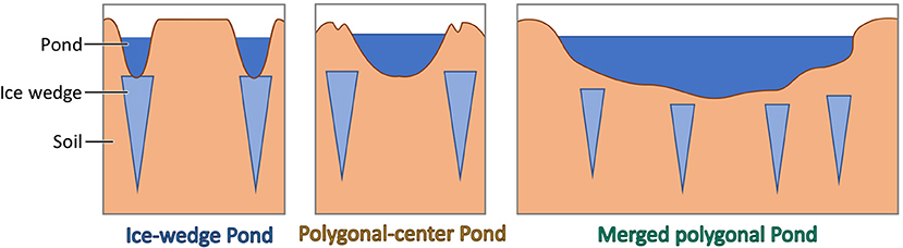
Figure 1. Schematic of the different pond types in the polygonal tundra. Ice-wedge ponds form along the edges of polygons on top of ice wedges, have a frozen bottom and have often an elongated shape and a steep slope. Polygonal-center ponds form in between ice wedges, in the center of the polygons. They tend to be nearly circular. If several polygons subside, merged polygonal ponds form. These ponds are the largest pond type of the three.

Polygonal tundra is prevalent throughout the lowlands of the Arctic, and often peatlands form in these patterned-ground landscapes characterized by a pronounced microrelief (French, 2007; Minayeva et al., 2016). Especially in the centers of the polygons, where the water table is higher than along the rims of the polygons, peat forms. These landscapes feature a high density of small waterbodies and carbon-rich soils. Here, we build on the work by Negandhi et al. (2013) and investigate what drives variability in methane concentrations of ponds in the polygonal tundra of Eastern Siberia. We include a wide range of variables, from wind speed over vegetation cover to geomorphological pond type. Notably, we also include the effect of submerged mosses on methane-concentration variability. These mosses photosynthesize and create an oxic zone at the bottom of the pond, where methane can be oxidized. This layer is often strongly enriched with methane, and concentrations drop steeply above the moss layer (Liebner et al., 2011; Knoblauch et al., 2015). Though these effects are known, it is unknown how submerged mosses impact methane concentrations on the scale of a whole pond.

2. Materials and Methods

2.1. Site Description

We studied 41 ponds on the islands Samoylov and Kurungakh (Figure 2). The two islands are located in the Lena River Delta of Eastern Siberia in a zone of continuous permafrost with an annual mean temperature of −12.5°C (Boike et al., 2013). The delta can be divided into three terraces of different genesis. The first terrace is the youngest, it formed in the Holocene through fluvial deposition. This terrace is the wettest, has the most pronounced microtopography due to active ice-wedge polygon formation and consequently the highest density of small-scale waterbodies (Schwamborn et al., 2002; Schneider et al., 2009; Muster et al., 2012). Both Samoylov and the southern tip of Kurungakh belong to the first terrace, and here we sampled 35 ponds in total. Six additional ponds were measured further north on Kurungnakh on the third terrace. The third terrace consists of sandy deposits overlain by an ice complex which formed in the Pleistocene. This organic-rich ice complex then is often overlain again by Holocene deposits (Schwamborn et al., 2002; Wetterich et al., 2008). The locations we sampled on the third terrace exhibited only weak polygonal structures, and especially smaller waterbodies were more sparse than on the first terrace. Still, overall roughly 20% percent of the delta (excluding the river) are covered by waterbodies—on the first terrace we find most small waterbodies while the third terrace has a higher fraction of large thermokarst lakes (Muster et al., 2012). The second terrace features less ponds and has not been sampled.

FIGURE 2

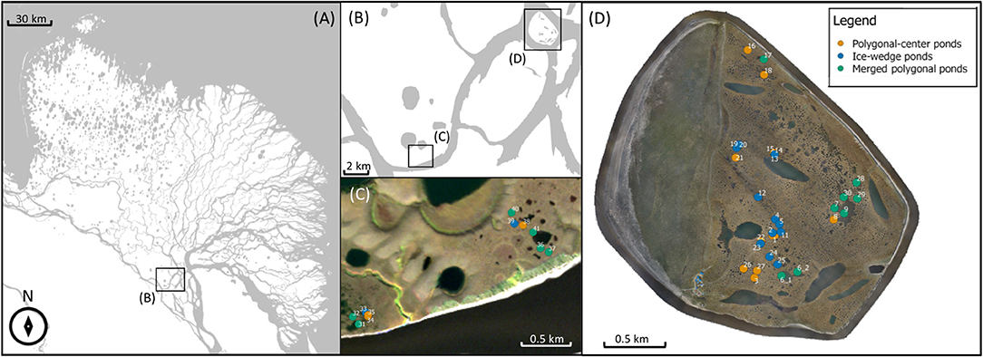
Figure 2. Overview of study region. The Lena River Delta (A) is located in Eastern Siberia at the coast of the Laptev Sea. Samoylov and Kurungakh Island are situated in the southern end of the Delta (B–D). Maps in (A,B) adapted from OpenStreetMap contributors, under Open Database License. Each dot represents one sampled pond (C,D).

We divided the waterbodies into three groups based on their geomorphology (Figure 1). Ponds which formed in the center of a single polygon with intact rims are labeled polygonal-center ponds. These ponds are mostly circular and only seldomly deeper than one meter. Ice-wedge ponds are ponds which formed on top of a thawing ice wedge along the edge of one or several polygons. These ponds tend to have an elongated shape and highly variable water depth with steep margins. Lastly, if several neighboring polygons including their rims are inundated, we call them merged polygonal ponds. These ponds are the largest and differ most in size. They also usually have the gentlest slope. We sampled 15 polygonal-center ponds with areas ranging from 24 to 200 m², 13 ice-wedge ponds with areas between 13 and 252 m², and 14 merged polygonal ponds (area range 214–24, 301 m²).

In the shallow parts and along the margins of all pond types, vascular plants species such as Carex aquatilis or Artcophila fulva grow (Knoblauch et al., 2015). On the bottom of many ponds, submerged brown mosses form a thick layer (Liebner et al., 2011; Knoblauch et al., 2015).

2.2. Gas Concentration Measurements

We conducted the field measurements on 22 days between mid-July and the end of August during mid-day to afternoon. In each pond several water samples were taken within an hour. The number of samples was dependent on ground-cover heterogeneity: The ground of a pond was either covered by vegetation like vascular plants or submerged mosses or vegetation free. For each pond, we took at least one sample over each ground-cover type, on average we took two samples. In total, we collected 116 surface water sample, 44 samples over sediment, 37 over moss, and 33 in the overgrown part of ponds. The overgrown fraction got sampled least, as it covers a smaller part of the average pond than mosses. Most samples were taken over sediment, because most of the area of larger ponds has bare ground. To get a better estimate by including more spatial variability, in large ponds surface concentrations over sediment were taken more than once. Water samples were taken through three aluminum tubes which were fixed to a larger 2 m pipe. To this pipe, two floating bodies were attached (see Supplementary Figure 1). We carefully placed the pipe in the pond away from the margin with little disturbance of the water. Up to three samples were taken at one spot within the pond: One five centimeters below the water surface through the first aluminum tube; one at the bottom of the pond through a second aluminum tube which end could be lowered; and, if the water was deeper than about half a meter, one additional sample was taken at about 55 cm depth through a third aluminum tube. Water was sucked through the respective tube with 50 mL syringes. After flushing the syringes, a 30 mL water sample was inserted into 50 mL injection bottles, which, beforehand, had been evacuated and then filled with nitrogen. The samples were stored dark between sampling and measuring to avoid photolysis and microbial breakup of dissolved organic carbon. The gas in the headspace of the injection bottles was analyzed within 12 h of sampling using a gas chromatograph (Agilent GC 7890, Agilent Technologies, Germany) with an flame ionization detector (FID). The headspace pressure in the injection bottle was measured with a digital manometer (LEO1, Keller, Switzerland). We estimate a loss of methane due to oxidation between sampling and gas chromatography measurement well below 5%. For this estimate, we use the mean potential methane oxidation rate for Alaskan non-yedoma lakes as determined by Martinez-Cruz et al. (2015) and the approach of the same authors to infer the in-situ oxidation rates by a double Monod model.

We computed the methane and carbon dioxide concentrations using the measured partial pressure of the respective gas in the headspace of the injection bottle, the ideal gas law and Henry's law with a temperature-dependent Henry's constant (Sander, 2015). The gas content of each injection bottle was measured at least twice.

2.3. Environmental Sampling

Using the handheld meter WTW Multi 340i (Xylem Analytics, Germany) and, on the last day of measurements, a WTW Multi 350i, equipped with a CellOx325 probe we measured dissolved oxygen in the pond water and water temperature with a SenTix41 probe. After each water sampling, we estimated the thaw depth of the ponds by driving a metal rod into the sediment until it hits the frozen ground. To assess water depth, we submerged a water-level logger Mini-Diver (DI501, Schlumberger Water Services, Netherlands) in the middle of the ponds. This diver measured temperature and hydrostatic pressure. Using a second diver which measured atmospheric pressure and the difference between the hydrostatic and atmospheric pressure, we computed water depth.

In each pond, we collected two subaquatic top-sediment samples near the shore. The sediment sampling was done directly after the water sampling. According to Knoblauch et al. (2015), the top sediment exhibits higher methane production rates than deeper soil layers. We removed large roots from the samples, dried the sample for 24 h at 105°C and measured the sample mass. We then determined the organic fraction of the sample by burning it in a muffle furnace for 4 h at 550°C and remeasuring the mass.

For incoming short-wave radiation, data from a four-component net radiation sensor (NR01, Campell Scientific, UK) was used. Wind speed was measured with a omnidirectional ultrasonic anemometer (R3-50, Gill Instruments, UK). Both of these instruments were stationary installed on Samoylov Island, data was recorded at half-hourly intervals.

2.4. Imagery

We used an orthophoto map of Samoylov and Kurungakh obtained in 2016 (Kartoziia, 2019) to determine the area of each pond, the area covered by moss and the area overgrown by plants. The map has a resolution of 0.05 m px⁻¹ thus providing enough detail to differentiate between surface types (see Figure 3). The orthophoto map was loaded into the GIS software ArcGIS 10.2.2, in which the ground-cover types were circled manually. The calculations of the enclosed areas were made in automatic mode in the GIS software QGIS. For very small ponds and for quality control, the areas computed through imaginary were compared to measurements of the pond diameter (see Supplementary Table 1) and to measurements of the width of the overgrown margin taken during the measurement campaign with a measuring tape. When possible, we also visually estimated the moss-covered fraction, to compare with the orthophoto map. For ponds, where the orthophoto map resolution was insufficient, the area approximated by the tape measurements was used.

FIGURE 3

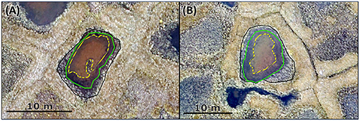
Figure 3. Excerpt of the orthophoto (Figure 2D) shows two exemplary polygonal-center ponds, panel (A) shows pond 3, panel (B) shows pond 21. Both are located on Samoylov Island. The black line marks the edge of the pond, the green line delimits the overgrown area, and the yellow dashed line marks the moss-covered parts of the pond.

2.5. Statistical Analysis

For each time a pond was measured (water and environmental sampling), we averaged all measurements of surface methane concentrations and computed the standard deviation. To assign a standard deviation to those ponds with only one sample, we performed a linear regression between the standard deviation and the mean concentration of the ponds with more than one sample (R² = 0.8) and used the regression to predict the standard deviation of the ponds with one sample.

As a measure of correlation we applied the Kendall rank correlation index (Knight, 1966). The advantage of this Kendall's tau is that it does not assume a linear relation between the two variables in question. This is achieved by always comparing a pair of two points: If both variables show the same trend (increase or decrease) between two points, it is counted toward the concordant pairs. If one variable shows an increase and the other a decrease, the pair is counted toward the discordant pairs. The index then is computed as the difference between the concordant and the discordant pairs divided by the absolute number of pairs while accounting for ties. Analogously to the more common Pearson correlation, an index of 1 indicates a strong positive correlation, −1 indicates a strong negative correlation, and 0 indicates no correlation.

To investigate the relation between methane concentrations and individual drivers in depth, we used linear regressions based on ordinary least squares, with log-transformed variables when looking at the relation between pond area and surface methane concentrations. To evaluate the goodness of the fit, we utilize the error on the slope parameter and the root mean squared error (RMSE) as well as the predictive R². The predictive R² gives a measure of how well the regression model predicts new observations. It is determined by removing one measurement from the dataset, redoing the regression and predicting the removed measurement. After repeating this procedure for all measurements in the dataset, the predictive R² is computed using the true and the predicted values of the target variable. The predictive R² is sensitive to overfitting.

To determine if two distributions are statistically different we used the Kolmogorov–Smirnov test (Hodges, 1958), which is a general, non-parametric test, which is sensitive both to the shape and to the location of a distribution. All analysis was done in python 3.6 using the packages numpy 1.17 (Harris et al., 2020), scipy 1.5 (Virtanen et al., 2020), scikit learn 0.21 (Pedregosa et al., 2011), and matplotlib 3.2 (Hunter, 2007).

2.6. Equilibrium Concentrations

The dissolved gas concentrations of methane and carbon dioxide for equilibrium conditions were computed using the mean measured water temperature, the mean air pressure, the mean atmospheric methane and carbon dioxide concentrations as measured by a nearby eddy-covariance station. Using a temperature-dependent Henry's constant H(T) (Sander, 2015), the concentrations were computed via

$\begin{array}{ll}c=H(T)·p,& (1)\end{array}$

where c is the equilibrium concentration in water, and p is the partial pressure (atmospheric pressure multiplied by the mole fraction of methane or carbon dioxide).

3. Results

Median concentrations in ice-wedge, polygonal-center and merged polygonal ponds, respectively, are 2.4 μmol L⁻¹ (25–75th percentile: 0.9–7.1 μmol L⁻¹), 0.6 μmol L⁻¹ (25–75th percentile: 0.4–1.5 μmol L⁻¹) and 0.7 μmol L⁻¹ (25–75th percentile: 0.5–1.2 μmol L⁻¹). All these values are far higher than the average methane equilibrium concentration of 0.004 μmol L⁻¹, which was computed using the mean water temperature of 9.7°C, mean air pressure of 101.144 kPa and mean methane air concentration of 2 ppm. Additionally, all ponds exhibited stratification. When comparing surface concentrations to bottom concentrations over sedimented areas in the ponds, where mixing is not obstructed, bottom concentrations in ice-wedge ponds are on average more than 100 times larger than surface concentrations. For polygonal-center ponds and merged polygonal ponds, bottom concentrations still exceed surface concentrations by a factor of 42 and 38 on average (see Table 1).

TABLE 1

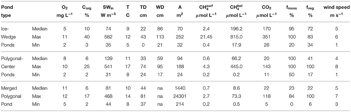
Table 1. Environmental conditions and geomorphological properties of the three pond types during the measurement campaign: dissolved oxygen (O₂), organic content in subaquatic topsoil (C_org), mean incoming shortwave radiation in the last 6 h before water sampling (SW_in), surface water temperature (T), thaw depth beneath the pond (TD), water depth (WD), area (A), bottom methane concentration (${\text{CH}}_4^{bot}$), surface carbon dioxide concentration (CO₂), moss-covered fraction of the pond surface (f_moss) fraction of pond overgrown by vascular plants (fveg) and the mean wind speed in the last 1.5 h before water sampling (wind speed).

3.1. Ice-Wedge Ponds

Ice-wedge ponds exhibit by far the highest methane concentrations and the largest spread in the distribution (Figure 4). In ice-wedge ponds, the surface concentrations tend to be low when wind speed is below 4 m s⁻¹ (Figure 5). In this regime, the pond is stratified because bottom temperatures are much lower than in the other two pond types [5.9(2.5) vs. 9.5(2.2)°C (mean with standard deviation)]. With raising wind speeds maximum surface concentrations steeply increase. The strength of this increase mainly correlates with the bottom concentrations. The more methane there is at the bottom, the more gets mixed up (Kendall-tau correlation between bottom and surface methane concentrations for all wind speeds: p < 0.05, for wind > 4 m s⁻¹:p < 0.01). Both the bottom and the surface methane concentrations significantly correlate solely to each other. The next-strongest correlation of the bottom concentrations is with area (p = 0.2). Using area, wind speed and bottom concentrations as regressors in a multiple linear regression, we achieve a predictive R² of 0.6.

FIGURE 4

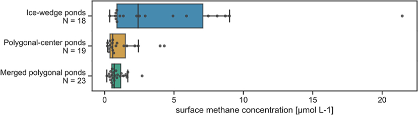
Figure 4. Distribution of surface concentrations separated by pond type. Boxplots with median as well as all data points are displayed. Number of measurements (N) is stated next to each boxplot.

FIGURE 5

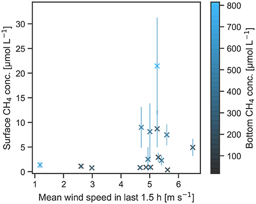
Figure 5. Surface methane concentrations of the ice-wedge ponds in relation to mean wind speed in the last 1.5 h and methane bottom concentrations.

3.2. Polygonal-Center Ponds

While area was a good predictor for ice-wedge ponds, water depth is more potent for polygonal-center ponds (Figure 6). Water depth and area do not significantly correlate for this pond type (p = 0.3). Apart from water depth, surface methane concentrations in polygonal-center ponds also significantly correlate with organic content in the top sediment, and these two are slightly correlated with each (p = 0.07) and both significantly correlated with the overgrown fraction (p < 0.05). Using the first principle component of these three variables as input for a linear regression on the surface concentrations yields a predictive R² of 0.6.

FIGURE 6

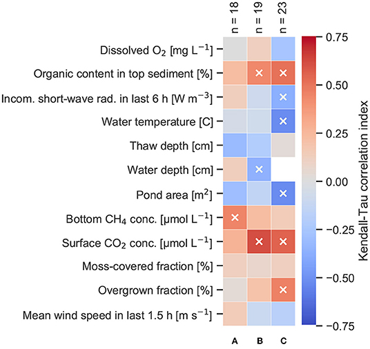
Figure 6. Kendall-Tau correlation index of different variables with surface methane concentrations in (A) ice-wedge ponds, (B) polygonal-center ponds, (C) merged polygonal ponds. Significant correlations (p < 0.05) are marked by a white cross. Number of measurements per pond type (n) is indicated at the top of each column.

3.3. Merged Polygonal Ponds

Polygonal-center and merged polygonal ponds have a similar range of methane surface concentrations, but merged polygonal ponds have the least skewed distribution among the three pond types (Figure 4). These ponds also correlate significantly to the largest number of environmental variables, like water temperature and incoming shortwave radiation (Figure 6). Using the first two principle components of the pond area, the overgrown fraction, the incoming shortwave radiation, dissolved oxygen and the organic content yields a predictive R² of 0.6.

3.4. Pond-Type Independent Results

The relation between surface methane concentration and pond area can be approximated by a log-log relation (Figure 7). While the relation between area and methane concentration for merged polygonal ponds is strongest among the three pond types ($R_{\mathrm{\text{pred}}}^2=0.21$), the deviation from the regression model increases for small ponds and no clear trend with area is visible. Compared to the linear regression, ice-wedge ponds have higher-than-expected concentrations, while polygonal-center ponds have lower-than-expected concentrations for a given area.

FIGURE 7

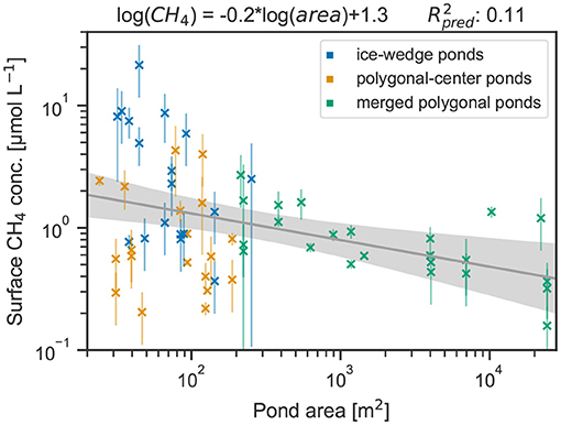
Figure 7. Linear regression between the natural logarithm of methane surface concentrations and the natural logarithm of pond area. Shaded area indicates the 95% confidence band.

The fraction covered by mosses has no clear influence on surface methane concentrations. For all three pond types, the error on the slope parameter of a linear regression between surface methane concentrations and moss cover is far larger than the slope parameter (see Supplementary Figure 2). This indicated that the sign of the regression can not be determined.

4. Discussion

The surface methane concentrations measured in this study fall in the range of concentrations measured on Samoylov Island before (Abnizova et al., 2012; Knoblauch et al., 2015). The concentrations in the polygonal tundra of the Lena River Delta are lower than the mean concentration of small ponds in the permafrost-affected parts of Western Siberian Lowlands (Polishchuk et al., 2018, 9 μmol L⁻¹). A large fraction of the West Siberian Lowlands is characterized by peatlands and many ponds and lakes formed through thermokarst. Only part of the West Siberian Lowlands is covered by polygonal tundra. A major difference between the two landscapes, which could explain the difference in concentrations, is the water depth of the ponds. The ponds in our study tend to be more than four times deeper (depths of ice-wedge and polygonal-center pond range from 17 to 117 cm) than ponds of the same area in the Western Siberian Lowlands (Polishchuk et al., 2018). When comparing to the more similar landscape of polygonal tundra in Northern Canada, we find that the concentrations and particularly the differences between the two small pond types match very well [Laurion et al., 2010; Negandhi et al., 2013, mean with standard deviation in parenthesis: ice-wedge ponds 4.1(4.7) μmol L⁻¹; polygonal-center ponds 1.3(1.7) μmol L⁻¹]. We can thus assume these concentration ranges hold as well for other regions that contain similar pond types, and that the drivers we identify here might apply in other regions, too. We find that the drivers and the distribution of methane concentrations differ between pond types.

4.1. Ice-Wedge Ponds

Surface methane concentrations in ice-wedge ponds can be reasonably well-predicted using area, wind speed and bottom concentrations. However, bottom concentrations in turn do not exhibit a correlation to any of the measured variables. This might be due to stratification, which we observe and has also been observed in ice-wedge ponds by Negandhi et al. (2014). We hypothesize that both bottom and surface concentrations depend on the current and past mixing efficiency, which determines the time methane accumulated in the hypolimnion. Because of this accumulation process, the dependency of bottom concentrations on other drivers, like substrate availability, could be masked. This decoupling between methane production and release has been observed by Sachs et al. (2008) in the polygonal tundra of Samoylov Island. Nevertheless, in Swedish lakes, Juutinen et al. (2009) found that bottom concentrations correlate with nutrient content. We might not capture this dependency in ice-wedge ponds because the organic content in the top sediment might not be representative for the substrate availability in this pond type: Koch et al. (2018) found that especially in newly-formed ice-wedge ponds old carbon leeches into the pond along the edge, which is consistent with results by Negandhi et al. (2013) and Laurion et al. (2010), who find that this pond type emits a larger fraction of old carbon compared to polygonal-center ponds. More of the methanogenesis might be fueled by this leaching of dissolved organic matter, which is a different substrate source than the organic content in the top sediment that was measured in this study. Negandhi et al. (2014) found methane produced from leached organic material to be slightly more abundant in ice-wedge than in polygonal-center ponds. Therefore, the negative dependence of surface methane concentrations in ice-wedge ponds on area could be driven by two mechanisms. First, gas-exchange velocities increase the larger the area of the pond is (Bastviken et al., 2004; Read et al., 2012; Negandhi et al., 2014), and, second, as ice-wedge pond formation is a type of permafrost degradation, the larger the pond, the more advanced is the degradation (Liljedahl et al., 2016). The more degraded the permafrost around the pond is, the less likely is it that labile old permafrost is leached. Reinforcing this, the larger the pond, the smaller the fraction of the pond bottom that is comprised of ice: we found that larger ponds have a deeper than average thaw depth (p < 0.05). To sum up, the typical features of ice-wedge ponds tend to be less pronounced the larger the area of an ice-wedge pond, and the ponds become more similar to polygonal-center ponds. The reverse effect can also be observed in Figure 7: The smaller the ice-wedge and polygonal center ponds are, the larger is the difference between their methane concentrations.

4.2. Polygonal-Center Ponds

Surface area and water depth of waterbodies regulate diffusive gas transport in a similar manner. The larger or the shallower the pond, the better mixed it is: Larger surface areas promote wind-induced mixing and thus a deeper mixed layer as well as a higher gas exchange velocity (Bastviken et al., 2004; Read et al., 2012). The deeper the pond, the longer the distance the gas has to travel from its source in the sediment to the surface. Though depth and area are often correlated (Wik et al., 2016), in our study, we find that water depth and area are hardly correlated for polygonal-center ponds (Figure 6). When comparing their relative importance, water depth has a stronger impact than area on surface methane concentrations in polygonal-center ponds. This is in line with Juutinen et al. (2009) and Wik et al. (2016) who found that generally for all waterbody types water depth is a better predictor of methane fluxes than area.

Instead of area, water depth in polygonal-center ponds is highly correlated with the overgrown fraction of the ponds in our study—wherever the water is shallow enough, plants tend to take root. Vascular plants also have a strong impact on the carbon cycling in ponds. For example, vascular plants are known to enhance methane emissions by acting as chimneys through which the methane produced at the sediments can bypass the oxidation zone (Kutzbach et al., 2004; Knoblauch et al., 2015). Further, vascular plants are known to increase substrate quality, consequently enhancing methanogenesis in the sediment (Joabsson and Christensen, 2001; Strom et al., 2003). This second effect might be the reason that ponds with the highest overgrown fraction also are likely to contain high organic fraction in the top sediment. Consequently, shallow polygonal-center ponds are mixed better and have a higher substrate availability as they are overgrown to a greater extent. Since we observe that out of the three drivers, which together well explain the variability of surface methane concentrations, two are connected to substrate availability, we conclude that polygonal-center ponds are substrate-limited. Additionally, the strongest driver of the variability between the ponds is due to variations in topography, primarily water depth.

4.3. Merged Polygonal Ponds

Compared to the other two pond types, merged polygonal ponds are the largest, the deepest and, consequently, the pond type with least moss cover and the smallest overgrown fraction. A larger surface area increases the gas-exchange velocities, and a vegetation-free pond bottom promotes faster upward mixing into the water column. Therefore, we hypothesize that the coupling between the production of methane in the sediment and surface methane concentrations is strongest in merged polygonal ponds among the pond types. The stratification of ice-wedge and polygonal-center ponds might at least partly mask the influence of environmental variables, like water temperature, on surface methane concentrations. Thus, that methane concentrations in merged polygonal ponds significantly correlate with the largest number of variables might be due to their better-mixed state. The negative correlation of methane surface concentrations with incoming solar radiation and water temperature has been observed before in a study by Burger et al. (2016) but stands in contrast to other studies (e.g., Yvon-Durocher et al., 2014; Natchimuthu et al., 2016; Jansen et al., 2020), which find that methane concentrations and fluxes increase with increasing temperatures. We cannot conclusively determine the mechanisms responsible for the negative correlation but offer several arguments. Warmer temperatures strengthen both methanogenesis, which increase surface methane concentrations, and the oxidation of methane in the water column, which decreases methane surface concentrations. Studies come to varying results regarding which of the two processes has a stronger temperature dependency (Duc et al., 2010; Borrel et al., 2011; Lofton et al., 2014; Negandhi et al., 2016). However, in Arctic soils methanogenesis is less temperature-dependent than in warmer regions as the methanogenic communities are adapted to cold temperatures (Tveit et al., 2015). Additionally, the merged polygonal ponds have the lowest overgrown fraction and the lowest fraction of organic content in the top sediment. The temperature dependence of the methanogenesis might also be dampened because of substrate limitation (Lofton et al., 2014; DelSontro et al., 2016), specifically as methanogenesis in the study area is known to depend on substrate quality (Wagner et al., 2003). At the same time, mainly when the ponds are deeper, the water temperature, which was used in the correlation analysis, can be assumed to be more variable than the sediment temperatures, which more directly affect methane concentrations. The methanotrophs benefit before the methanogens, when water warms. Ensuing temperature differences between water surface and sediment might also enhance stratification: Stratification slows down the transport of methane through the water by inhibiting turbulent mixing, and, if there is still oxygen in the water column, additionally enhances oxidation efficiency.

Rather than water temperature, the incoming radiation in the last 6 h is more likely the root cause of enhanced stratification, as a measure of how much energy got absorbed by the lake in the last 6 h. Supporting this, we find that incoming radiation predicts surface methane concentrations better than the water temperature for predicting surface methane concentrations in merged polygonal pond types together with dissolved oxygen, pond area, organic content in the top sediment and the overgrown fraction. Dissolved oxygen was measured close to the surface making this parameter an indicator of how well the surface layer is mixed and how much oxygen is available for methanotrophs. Both mixing and oxidation decrease methane surface concentrations. Overgrown area can, like for polygonal-center ponds, be seen as a proxy for both the substrate quality and the mean water depth. Especially as the organic content and the overgrown fraction of merged polygonal ponds are smaller than in polygonal-center ponds, we can analogously infer that merged polygonal ponds are substrate-limited and, more than polygonal-center ponds, dependent on those environmental conditions, which influence stratification. Lastly, we note that both stratification and vegetated fraction are at least partly regulated by the topography and mean water depth of the ponds.

4.4. Drivers of Methane Variability Between Pond Types

The three geomorphological pond types have varying drivers of type-internal methane variability, and concurrently, the distributions and mean values of surface methane concentrations of the three pond types differ as well.

Ice-wedge ponds are the most stratified and exhibit other bacterial communities than polygonal-center ponds (Negandhi et al., 2014); merged polygonal ponds are the largest, the best mixed pond type with the highest gas-exchange velocities (Bastviken et al., 2004; Read et al., 2012), and the pond type with the least substrate, the smallest overgrown and moss-covered fraction. Polygonal-center ponds are of the same size as ice-wedge ponds, but for many properties, like dissolved oxygen or thaw depth, fall into the middle of the other two ponds. A reason why the surface methane concentrations of polygonal-center ponds are not as high as would be expected from the log-log regression between methane concentrations and area (see Figure 7) might lie with water depth. In polygonal-center ponds, surface methane concentrations strongly depend on water depth, but water depth is not strongly correlated with area. Thus, though polygonal-center ponds have a smaller area than merged polygonal ponds, they might not be shallower.

4.4.1. Area

As previous studies (DelSontro et al., 2018; Zabelina et al., 2020) suggest, we find that pond area alone is not sufficient to explain variability in methane concentrations. Yet, the observed trend is in agreement with prior studies (Juutinen et al., 2009; Wik et al., 2016), and the relation between pond size and methane concentrations is very similar to the estimate by Polishchuk et al. (2018)—their regression line follows log([CH₄]) = −0.258 · log(area) + 0.635. This similarity especially in the slope (our result: −0.2) is astounding since Polishchuk et al. (2018) covered a much larger spatial area, spanning from continuous to sporadic permafrost zones. We conclude that, especially for ponds larger than roughly 10 m², an area-based upscaling can be a reasonable choice in permafrost-affected landscapes, but that for smaller ponds additional predictors need to be taken into consideration.

4.4.2. Moss Cover

Most of the subaquatic soils of the ponds in the study area are at least partly covered by submerged mosses (Scorpidium scorpioides). This moss photosynthesizes at the bottom of the pond and creates an oxic layer where methane can be oxidized. Additionally, the thick moss captures bubbles and thus suppresses ebullition (Liebner et al., 2011; Knoblauch et al., 2015). Surprisingly, we do not find that moss cover reduces surface methane concentration on the pond scale (Supplementary Figure 2). However, we find that moss does inhibit diffusion, if we look at stratification: Bottom methane concentrations in the moss layer are on average (with standard deviation) 1.8(1.2) times higher than in open water. To reconcile these two findings, we hypothesize that moss cover has a counterbalancing effect: If moss also enhances methanogenesis by providing additional organic substrate similar to what has been shown for vascular plants (Joabsson and Christensen, 2001; Strom et al., 2003), then even though moss leads to enhanced oxidation at the bottom of the pond, the higher productivity might balance out the loss through oxidation. Additionally, the accumulation of methane in the moss layer creates a gradient between moss-covered and moss-free areas in the ponds which are not completely covered by moss. Through lateral mixing part of the methane might escape the moss layer and reach the surface.

The mosses in our study area should not be confused with mosses of the genus Sphagnum. Kuhn et al. (2018) found that for sphagnum-dominated ponds diffusive methane fluxes are lower than for ponds with open water, but in contrast to the submerged mosses in our study side, Sphagnum stays at the water surface, and thus has a direct impact on the gas exchange at the water-air interface.

4.4.3. Carbon Dioxide

All ponds show a positive correlation between surface methane and carbon dioxide concentrations (Figure 6). This correlation was expected, since carbon dioxide is produced during acetoclastic methanogenesis, which is assumed to be the most prominent pathway of methanogenesis in cold lakes and ponds (Borrel et al., 2011; Negandhi et al., 2013; Tveit et al., 2015). Additional carbon dioxide is produced during the oxidation of methane, and the oxidation rates have been found to be coupled to methane production rates (Duc et al., 2010). Thus, at least part of the production of carbon dioxide in the pond is closely coupled to methanogenesis. Additionally, the carbon dioxide produced independently of the methane might follow similar drivers.

5. Conclusions

The dominant drivers of methane emissions differ depending on the pond type. We consider substrate availability to be an important driver of methane concentrations markedly in polygonal-center and merged polygonal ponds. Smaller, shallower ponds tend to be richer in substrate (more organic content in the sediment and higher overgrown fraction) and thus exhibit higher concentrations. Accordingly, substrate availability is at least partly determined by the topography of the pond. This finding matches results from prior studies (Juutinen et al., 2009; Sepulveda-Jauregui et al., 2015). The easiest-to-measure topographical property of ponds is area, and, for merged polygonal ponds, area is a good predictor of methane concentrations. But for polygonal-center ponds, water depth is a far better predictor. Water depth, overgrown fraction (as both a proxy for mean water depth and for substrate availability) and organic fraction in the top sediment are enough to predict surface methane concentrations reasonably well in polygonal-center ponds. In our study, the incoming short-wave radiation over the past 6 h was the best proxy for stratification, much improving the statistical model for merged polygonal ponds.

Lastly, ice-wedge ponds are the most distinct pond type. Ice-wedge ponds are strongly stratified as they are narrow, steep and feature a large temperature gradient in summer. If bottom waters are mixed up, surface methane concentrations spike. Additionally, these ponds tend to be richer in substrate and have been shown to emit a larger fraction of old carbon than polygonal-center ponds (Laurion et al., 2010; Negandhi et al., 2013). We find that ice-wedge ponds feature the highest concentrations and, thus, likely also the highest diffusive emissions.

We do not find that the moss-covered fraction of a pond controls methane surface concentrations, as moss might enhance local methanogenesis by providing substrate and lateral mixing might reduce the dampening effect of moss on diffusion.

Climate changes at an above-average rate in the Arctic, and there is growing evidence that global warming will enhance methane emissions from ponds (e.g., Tan and Zhuang, 2015; Vonk et al., 2015; Wik et al., 2016; Aben et al., 2017; Yvon-Durocher et al., 2017), especially so from ice-wedge ponds, which are expected to increasingly form (Liljedahl et al., 2016; Martin et al., 2017). When including small waterbodies in large-scale studies, it is import to choose an appropriate representation for the ponds. As it is not possible to approximate the behavior of all pond types in our study with the same drivers, let alone use a single driver to approximate the behavior of all ponds, we conclude that process-based models which ideally capture the different waterbody types will be useful in the improvement of upscaling of pan-Arctic waterbody-methane emissions.

Data Availability Statement

The data has been published at: https://doi.pangaea.de/10.1594/PANGAEA.922399 (Rehder et al., 2020).

Author Contributions

ZR: conceptualization (equal), formal analysis (lead), investigation (lead), and writing - original draft. AZ: formal analysis (supporting) and investigation (supporting). LK: conceptualization (equal), formal analysis (supporting), and writing - review and editing. All authors contributed to the article and approved the submitted version.

Funding

This study was partly funded by the Deutsche Forschungsgemeinschaft (DFG, German Research Foundation) under Germany's Excellence Strategy—EXC 2037 CLICCS - Climate, Climatic Change, and Society—Project Number: 390683824, contribution to the Center for Earth System Research and Sustainability (CEN) of Universität Hamburg.

Conflict of Interest

The authors declare that the research was conducted in the absence of any commercial or financial relationships that could be construed as a potential conflict of interest.

The handling editor declared a past co-authorship with one of the authors LK.

Acknowledgments

The authors thank Norman Rüggen for his tireless support before and remotely during the fieldwork, Andrei Astapov, Waldemar Schneider, and Andrei Kartoziia for their equally tireless support in the field, Victor Brovkin and Thomas Kleinen for the helpful discussions on the analysis, and last but not least David Holl for his valuable suggestions on the manuscript. The authors also thank Sophia Burke and Ronny Lauerwald for their kind and helpful review.

Supplementary Material

The Supplementary Material for this article can be found online at: https://www.frontiersin.org/articles/10.3389/feart.2021.617662/full#supplementary-material

References

Aben, R. C. H., Barros, N., van Donk, E., Frenken, T., Hilt, S., Kazanjian, G., et al. (2017). Cross continental increase in methane ebullition under climate change. Nat. Commun. 8, 1–8. doi: 10.1038/s41467-017-01535-y

PubMed Abstract | CrossRef Full Text | Google Scholar

Abnizova, A., Siemens, J., Langer, M., and Boike, J. (2012). Small ponds with major impact: the relevance of ponds and lakes in permafrost landscapes to carbon dioxide emissions. Glob. Biogeochem. Cycles 26, 1–9. doi: 10.1029/2011GB004237

CrossRef Full Text | Google Scholar

Anderson, N. J., Harriman, R., Ryves, D. B., and Patrick, S. T. (2001). Dominant factors controlling variability in the ionic composition of west greenland lakes. Arctic Antarctic Alpine Res. 33, 418–425. doi: 10.1080/15230430.2001.12003450

CrossRef Full Text | Google Scholar

Bastviken, D., Cole, J., Pace, M., and Tranvik, L. (2004). Methane emissions from lakes: dependence of lake characteristics, two regional assessments, and a global estimate. Glob. Biogeochem. Cycles 18, 1–12. doi: 10.1029/2004GB002238

CrossRef Full Text | Google Scholar

Boike, J., Kattenstroth, B., Abramova, K., Bornemann, N., Chetverova, A., Fedorova, I., et al. (2013). Baseline characteristics of climate, permafrost and land cover from a new permafrost observatory in the lena river delta, siberia (1998-2011). Biogeosciences 10, 2105–2128. doi: 10.5194/bg-10-2105-2013

CrossRef Full Text | Google Scholar

Borrel, G., Jezequel, D., Biderre-Petit, C., Morel-Desrosiers, N., Morel, J. P., Peyret, P., et al. (2011). Production and consumption of methane in freshwater lake ecosystems. Res. Microbiol. 162, 832–847. doi: 10.1016/j.resmic.2011.06.004

PubMed Abstract | CrossRef Full Text | Google Scholar

Burger, M., Berger, S., Spangenberg, I., and Blodau, C. (2016). Summer fluxes of methane and carbon dioxide from a pond and floating mat in a continental Canadian peatland. Biogeosciences 13, 3777–3791. doi: 10.5194/bg-13-3777-2016

CrossRef Full Text | Google Scholar

Burpee, B., Saros, J. E., Northington, R. M., and Simon, K. S. (2016). Microbial nutrient limitation in arctic lakes in a permafrost landscape of southwest greenland. Biogeosciences 13, 365–374. doi: 10.5194/bg-13-365-2016

CrossRef Full Text | Google Scholar

DelSontro, T., Beaulieu, J. J., and Downing, J. A. (2018). Greenhouse gas emissions from lakes and impoundments: upscaling in the face of global change. Limnol. Oceanogr. Lett. 3, 64–75. doi: 10.1002/lol2.10073

PubMed Abstract | CrossRef Full Text | Google Scholar

DelSontro, T., Boutet, L., St-Pierre, A., del Giorgio, P. A., and Prairie, Y. T. (2016). Methane ebullition and diffusion from northern ponds and lakes regulated by the interaction between temperature and system productivity. Limnol. Oceanogr. 61, S62–S77. doi: 10.1002/lno.10335

CrossRef Full Text | Google Scholar

Downing, J. A. (2010). Emerging global role of small lakes and ponds: little things mean a lot. Limnetica 29, 9–23. doi: 10.23818/limn.29.02

CrossRef Full Text | Google Scholar

Duc, N., Crill, P., and Bastviken, D. (2010). Implications of temperature and sediment characteristics on methane formation and oxidation in lake sediments. Biogeochemistry 100, 185–196. doi: 10.1007/s10533-010-9415-8

CrossRef Full Text | Google Scholar

French, H. M. (2007). The Periglacial Environment, 3rd Edn. Chichester: John Wiley &Sons, Ltd. doi: 10.1002/9781118684931

CrossRef Full Text | Google Scholar

Hamilton, P. B., Gajewski, K., Atkinson, D. E., and Lean, D. R. S. (2001). Physical and chemical limnology of 204 lakes from the canadian arctic archipelago. Hydrobiologia 457, 133–148. doi: 10.1023/A:1012275316543

CrossRef Full Text | Google Scholar

Harris, C. R., Millman, K. J., van der Walt, S. J., Gommers, R., Virtanen, P., Cournapeau, D., et al. (2020). Array programming with numpy. Nature 585, 357–362. doi: 10.1038/s41586-020-2649-2

CrossRef Full Text | Google Scholar

Hodges, J. (1958). The significance probability of the smirnov two-sample test. Arkiv för Matematik 3, 469–486. doi: 10.1007/BF02589501

CrossRef Full Text | Google Scholar

Holgerson, M. A., and Raymond, P. A. (2016). Large contribution to inland water co2 and ch4 emissions from very small ponds. Nat. Geosci. 9, 222–226. doi: 10.1038/ngeo2654

CrossRef Full Text | Google Scholar

Hunter, J. D. (2007). Matplotlib: a 2d graphics environment. Comput. Sci. Eng. 9, 90–95. doi: 10.1109/MCSE.2007.55

CrossRef Full Text | Google Scholar

Jansen, J., Thornton, B. F., Cortés, A., Snöälv, J., Wik, M., MacIntyre, S., et al. (2020). Drivers of diffusive ch4 emissions from shallow subarctic lakes on daily to multi-year timescales. Biogeosciences 17, 1911–1932. doi: 10.5194/bg-17-1911-2020

CrossRef Full Text | Google Scholar

Joabsson, A., and Christensen, T. R. (2001). Methane emissions from wetlands and their relationship with vascular plants: an arctic example. Glob. Change Biol. 7, 919–932. doi: 10.1046/j.1354-1013.2001.00044.x

CrossRef Full Text | Google Scholar

Juutinen, S., Rantakari, M., Kortelainen, P., Huttunen, J. T., Larmola, T., Alm, J., et al. (2009). Methane dynamics in different boreal lake types. Biogeosciences 6, 209–223. doi: 10.5194/bg-6-209-2009

CrossRef Full Text | Google Scholar

Kartoziia, A. (2019). Assessment of the ice wedge polygon current state by means of UAV imagery analysis (Samoylov island, the Lena delta). Remote Sens. 11:1627. doi: 10.3390/rs11131627

CrossRef Full Text | Google Scholar

Knight, W. R. (1966). A computer method for calculating Kendall's tau with ungrouped data. J. Am. Stat. Assoc. 61, 436–439. doi: 10.1080/01621459.1966.10480879

CrossRef Full Text | Google Scholar

Knoblauch, C., Spott, O., Evgrafova, S., Kutzbach, L., and Pfeiffer, E. M. (2015). Regulation of methane production, oxidation, and emission by vascular plants and bryophytes in ponds of the northeast siberian polygonal tundra. J. Geophys. Res. Biogeosci. 120, 2525–2541. doi: 10.1002/2015JG003053

CrossRef Full Text | Google Scholar

Koch, J. C., Jorgenson, M. T., Wickland, K. P., Kanevskiy, M., and Striegl, R. (2018). Ice wedge degradation and stabilization impact water budgets and nutrient cycling in arctic trough ponds. J. Geophys. Res. Biogeosci. 123, 2604–2616. doi: 10.1029/2018JG004528

CrossRef Full Text | Google Scholar

Kuhn, M., Lundin, E. J., Giesler, R., Johansson, M., and Karlsson, J. (2018). Emissions from thaw ponds largely offset the carbon sink of northern permafrost wetlands. Sci. Rep/ 8, 1–7. doi: 10.1038/s41598-018-27770-x

PubMed Abstract | CrossRef Full Text | Google Scholar

Kutzbach, L., Wagner, D., and Pfeiffer, E. M. (2004). Effect of microrelief and vegetation on methane emission from wet polygonal tundra, Lena delta, northern Siberia. Biogeochemistry 69, 341–362. doi: 10.1023/B:BIOG.0000031053.81520.db

CrossRef Full Text | Google Scholar

Laurion, I., Vincent, W. F., MacIntyre, S., Retamal, L., Dupont, C., Francus, P., et al. (2010). Variability in greenhouse gas emissions from permafrost thaw ponds. Limnol. Oceanogr. 55, 115–133. doi: 10.4319/lo.2010.55.1.0115

CrossRef Full Text | Google Scholar

Liebner, S., Zeyer, J., Wagner, D., Schubert, C., Pfeiffer, E. M., and Knoblauch, C. (2011). Methane oxidation associated with submerged brown mosses reduces methane emissions from siberian polygonal tundra. J. Ecol. 99, 914–922. doi: 10.1111/j.1365-2745.2011.01823.x

CrossRef Full Text | Google Scholar

Liljedahl, A. K., Boike, J., Daanen, R. P., Fedorov, A. N., Frost, G. V., Grosse, G., et al. (2016). Pan-arctic ice-wedge degradation in warming permafrost and its influence on tundra hydrology. Nat. Geosci. 9:312. doi: 10.1038/ngeo2674

CrossRef Full Text | Google Scholar

Lofton, D. D., Whalen, S. C., and Hershey, A. E. (2014). Effect of temperature on methane dynamics and evaluation of methane oxidation kinetics in shallow Arctic Alaskan lakes. Hydrobiologia 721, 209–222. doi: 10.1007/s10750-013-1663-x

CrossRef Full Text | Google Scholar

Martin, A. F., Lantz, T. C., and Humphreys, E. R. (2017). Ice wedge degradation and Co2 and Ch4 emissions in the Tuktoyaktuk coastlands, northwest territories. Arctic Sci. 4, 130–145. doi: 10.1139/AS-2016-0011

CrossRef Full Text | Google Scholar

Martinez-Cruz, K., Sepulveda-Jauregui, A., Walter Anthony, K., and Thalasso, F. (2015). Geographic and seasonal variation of dissolved methane and aerobic methane oxidation in alaskan lakes. Biogeosciences 12, 4595–4606. doi: 10.5194/bg-12-4595-2015

CrossRef Full Text | Google Scholar

Minayeva, T., Sirin, A., Kershaw, P., and Bragg, O. (2016). Arctic Peatlands. Dordrecht: Springer. doi: 10.1007/978-94-007-6173-5_109-1

CrossRef Full Text | Google Scholar

Muster, S., Langer, M., Heim, B., Westermann, S., and Boike, J. (2012). Subpixel heterogeneity of ice-wedge polygonal tundra: a multi-scale analysis of land cover and evapotranspiration in the lena river delta, siberia. Tellus Ser. B Chem. Phys. Meteorol. 64. doi: 10.3402/tellusb.v64i0.17301

CrossRef Full Text | Google Scholar

Muster, S., Roth, K., Langer, M., Lange, S., Aleina, F. C., Bartsch, A., et al. (2017). Perl: a circum-arctic permafrost region pond and lake database. Earth Syst. Sci. Data 9, 317–348. doi: 10.5194/essd-9-317-2017

CrossRef Full Text | Google Scholar

Natchimuthu, S., Sundgren, I., Galfalk, M., Klemedtsson, L., Crill, P., Danielsson, A., et al. (2016). Spatio-temporal variability of lake ch4 fluxes and its influence on annual whole lake emission estimates. Limnol. Oceanogr. 61, S13–S26. doi: 10.1002/lno.10222

CrossRef Full Text | Google Scholar

Negandhi, K., Laurion, I., and Lovejoy, C. (2014). Bacterial communities and greenhouse gas emissions of shallow ponds in the high arctic. Polar Biol. 37, 1669–1683. doi: 10.1007/s00300-014-1555-1

CrossRef Full Text | Google Scholar

Negandhi, K., Laurion, I., and Lovejoy, C. (2016). Temperature effects on net greenhouse gas production and bacterial communities in arctic thaw ponds. FEMS Microbiol. Ecol. 92, 1–12. doi: 10.1093/femsec/fiw117

PubMed Abstract | CrossRef Full Text | Google Scholar

Negandhi, K., Laurion, I., Whiticar, M. J., Galand, P. E., Xu, X. M., and Lovejoy, C. (2013). Small thaw ponds: an unaccounted source of methane in the Canadian high Arctic. PLoS ONE 8:e78204. doi: 10.1371/journal.pone.0078204

PubMed Abstract | CrossRef Full Text | Google Scholar

Ortiz-Llorente, M. J., and Alvarez-Cobelas, M. (2012). Comparison of biogenic methane emissions from unmanaged estuaries, lakes, oceans, rivers and wetlands. Atmos. Environ. 59, 328–337. doi: 10.1016/j.atmosenv.2012.05.031

CrossRef Full Text | Google Scholar

Pedregosa, F., Varoquaux, G., Gramfort, A., Michel, V., Thirion, B., Grisel, O., et al. (2011). Scikit-learn: machine learning in python. J. Mach. Learn. Res. 12, 2825–2830.

Google Scholar

Polishchuk, Y. M., Bogdanov, A. N., Muratov, I. N., Polishchuk, V. Y., Lim, A., Manasypov, R. M., et al. (2018). Minor contribution of small thaw ponds to the pools of carbon and methane in the inland waters of the permafrost-affected part of the western siberian lowland. Environ. Res. Lett. 13:15. doi: 10.1088/1748-9326/aab046

CrossRef Full Text | Google Scholar

Ramsar Convention Secretariat (2016). An Introduction to the Ramsar Convention on Wetlands (previously The Ramsar Convention Manual). Ramsar Convention Secretariat, Gland.

Google Scholar

Read, J. S., Hamilton, D. P., Desai, A. R., Rose, K. C., MacIntyre, S., Lenters, J. D., et al. (2012). Lake-size dependency of wind shear and convection as controls on gas exchange. Geophys. Res. Lett. 39, 1–5. doi: 10.1029/2012GL051886

CrossRef Full Text | Google Scholar

Rehder, Z., Zaplavnova, A., and Kutzbach, L. (2020). Dissolved-Gas Concentrations, Physical and Chemical Properties of 41 Ponds as well as Key Meteorological Parameters in the Lena River Delta, Siberia. Pangaea.

Google Scholar

Rinta, P., Bastviken, D., Schilder, J., Van Hardenbroek, M., Stotter, T., and Heiri, O. (2017). Higher late summer methane emission from central than northern European lakes. J. Limnol. 76, 52–67. doi: 10.4081/jlimnol.2016.1475

CrossRef Full Text | Google Scholar

Sachs, T., Wille, C., Boike, J., and Kutzbach, L. (2008). Environmental controls on ecosystem-scale Ch4 emission from polygonal tundra in the Lena river delta, Siberia. J. Geophys. Res. Biogeosci. 113, 1–12. doi: 10.1029/2007JG000505

CrossRef Full Text | Google Scholar

Sander, R. (2015). Compilation of Henry's law constants (version 4.0) for water as solvent. Atmos. Chem. Phys. 15, 4399–4981. doi: 10.5194/acp-15-4399-2015

CrossRef Full Text | Google Scholar

Schneider, J., Grosse, G., and Wagner, D. (2009). Land cover classification of tundra environments in the Arctic Lena delta based on landsat 7 etm+ data and its application for upscaling of methane emissions. Remote Sens. Environ. 113, 380–391. doi: 10.1016/j.rse.2008.10.013

CrossRef Full Text | Google Scholar

Schwamborn, G., Rachold, V., and Grigoriev, M. N. (2002). Late quaternary sedimentation history of the lena delta. Q. Int. 89, 119–134. doi: 10.1016/S1040-6182(01)00084-2

CrossRef Full Text | Google Scholar

Sepulveda-Jauregui, A., Anthony, K. M. W., Martinez-Cruz, K., Greene, S., and Thalasso, F. (2015). Methane and carbon dioxide emissions from 40 lakes along a north-south latitudinal transect in Alaska. Biogeosciences 12, 3197–3223. doi: 10.5194/bg-12-3197-2015

CrossRef Full Text | Google Scholar

Strom, L., Ekberg, A., Mastepanov, M., and Christensen, T. R. (2003). The effect of vascular plants on carbon turnover and methane emissions from a tundra wetland. Glob. Change Biol. 9, 1185–1192. doi: 10.1046/j.1365-2486.2003.00655.x

CrossRef Full Text | Google Scholar

Tan, Z. L., and Zhuang, Q. L. (2015). Methane emissions from Pan-Arctic lakes during the 21st century: an analysis with process-based models of lake evolution and biogeochemistry. J. Geophys. Res. Biogeosci. 120, 2641–2653. doi: 10.1002/2015JG003184

CrossRef Full Text | Google Scholar

Tveit, A. T., Urich, T., Frenzel, P., and Svenning, M. M. (2015). Metabolic and trophic interactions modulate methane production by arctic peat microbiota in response to warming. Proc. Natl. Acad. Sci. U.S.A. 112, E2507–E2516. doi: 10.1073/pnas.1420797112

PubMed Abstract | CrossRef Full Text | Google Scholar

Virtanen, P., Gommers, R., Oliphant, T. E., Haberland, M., Reddy, T., Cournapeau, D., et al. (2020). Scipy 1.0: fundamental algorithms for scientific computing in python. Nat. Methods 17, 261–272. doi: 10.1038/s41592-019-0686-2

PubMed Abstract | CrossRef Full Text | Google Scholar

Vonk, J. E., Tank, S. E., Bowden, W. B., Laurion, I., Vincent, W. F., Alekseychik, P., et al. (2015). Reviews and syntheses: effects of permafrost thaw on arctic aquatic ecosystems. Biogeosciences 12, 7129–7167. doi: 10.5194/bg-12-7129-2015

CrossRef Full Text | Google Scholar

Wagner, D., Kobabe, S., Pfeiffer, E. M., and Hubberten, H. W. (2003). Microbial controls on methane fluxes from a polygonal tundra of the Lena delta, Siberia. Permafrost Periglacial Process. 14, 173–185. doi: 10.1002/ppp.443

CrossRef Full Text | Google Scholar

Wetterich, S., Schirrmeister, L., Meyer, H., Viehberg, F. A., and Mackensen, A. (2008). Arctic freshwater ostracods from modern periglacial environments in the Lena river delta (Siberian Arctic, Russia): geochemical applications for palaeoenvironmental reconstructions. J. Paleolimnol. 39, 427–449. doi: 10.1007/s10933-007-9122-1

CrossRef Full Text | Google Scholar

Wik, M., Varner, R. K., Anthony, K. W., MacIntyre, S., and Bastviken, D. (2016). Climate-sensitive northern lakes and ponds are critical components of methane release. Nat. Geosci. 9:99. doi: 10.1038/ngeo2578

CrossRef Full Text | Google Scholar

Yvon-Durocher, G., Allen, A. P., Bastviken, D., Conrad, R., Gudasz, C., St-Pierre, A., et al. (2014). Methane fluxes show consistent temperature dependence across microbial to ecosystem scales. Nature 507, 488–491. doi: 10.1038/nature13164

PubMed Abstract | CrossRef Full Text | Google Scholar

Yvon-Durocher, G., Hulatt, C. J., Woodward, G., and Trimmer, M. (2017). Long-term warming amplifies shifts in the carbon cycle of experimental ponds. Nat. Clim. Change 7:209. doi: 10.1038/nclimate3229

CrossRef Full Text | Google Scholar

Zabelina, S. A., Shirokova, L. S., Klimov, S. I., Chupakov, A. V., Lim, A. G., Polishchuk, Y. M., et al. (2020). Carbon emission from thermokarst lakes in ne european tundra. Limnol. Oceanogr. 66, S216–S230. doi: 10.1002/lno.11560

CrossRef Full Text | Google Scholar