 William P. Meurer
 John Blum
 Greg Shipman
- Reservoir Systems, Research and Technology Development, ExxonMobil Upstream Research Company, Spring, TX, United States
The role of methane as a green-house gas is widely recognized and has sparked considerable efforts to quantify the contribution from natural methane sources including submarine seeps. A variety of techniques and approaches have been directed at quantifying methane fluxes from seeps from just below the sediment water interface all the way to the ocean atmosphere interface. However, there have been no systematic efforts to characterize the amount and distribution of dissolved methane around seeps. This is critical to understanding the fate of methane released from seeps and its role in the submarine environment. Here we summarize the findings of two field studies of the Bush Hill mud volcano (540 m water depth) located in the Gulf of Mexico. The studies were carried out using buoyancy driven gliders equipped with methane sensors for near real time in situ detection. One glider was equipped with an Acoustic Doppler Current Profiler (ADCP) for simultaneous measurement of currents and methane concentrations. Elevated methane concentrations in the water column were measured as far away as 2 km from the seep source and to a height of about 100 m above the seep. Maximum observed concentrations were ∼400 nM near the seep source and decreased away steadily in all directions from the source. Weak and variable currents result in nearly radially symmetric dispersal of methane from the source. The persistent presence of significant methane concentrations in the water column points to a persistent methane seepage at the seafloor, that has implications for helping stabilize exposed methane hydrates. Elevated methane concentrations in the water column, at considerable distances away from seeps potentially support a much larger methane-promoted biological system than is widely appreciated.
Introduction
The importance of methane, leaked from the seafloor at seeps, as a food source in the deep oceans supporting complex biological communities is well documented (e.g., Kennicutt et al., 1988a; MacDonald et al., 1989; Sibuet and Olu, 1998; Sibuet and Roy, 2002; Cordes et al., 2005; Levin, 2005; Girard et al., 2020). Studies of these seep communities typically focus on megafaunal communities and microbial mats found close to release points on the seafloor. Recent work suggests that even modest dissolved methane concentrations (∼20 nM) can be important for microbial methane oxidizers (Uhlig et al., 2018) and may help to support the benthic communities at large (Åström et al., 2017). However, the relationship between the distribution of dissolved methane around seeps and any associated biological communities is poorly documented; likely because of limited sampling.
The study of the release of methane from thermogenic and biogenic seeps in the world’s oceans (and lakes) has expanded from simple recognition of the extent of the sources to efforts to characterize methane release mechanisms and quantify fluxes. These efforts include studies of: the exchange across the sediment water interface (Tryon and Brown, 2004; Kastner and MacDonald, 2006), bubble fluxes using bottom imaging (Leifer and MacDonald, 2003; Leifer, 2010; Thomanek et al., 2010; Römer et al., 2019; Di et al., 2020; Johansen et al., 2020), bubble fluxes using acoustic imaging (Weber et al., 2014), dissociation of hydrates (Lapham et al., 2010; Lapham et al., 2014), and inferred fluxes to the seafloor based on shallow thermal gradients (Smith et al., 2014). We now know that methane bubble release rates can vary on time scales of seconds, minutes, hours, and days (e.g., Greinert 2008; Leifer, 2019 (and references therein); Johansen et al., 2020). These flux variations can include times when no appreciable methane bubbles are released at all. The release point on the seafloor can also shift location on time scales of days (Razaz et al., 2020).
In contrast to the study of methane bubble releases, substantially less effort has been paid to understanding the distribution of dissolved hydrocarbons around seeps. Shipboard hydrocasts are commonly used to provide at most tens of samples of the water column around seeps. They provide point data in time and space and cannot effectively sample methane plumes without additional context. Manned submersibles and remotely operated vehicles have also been used to collect water-column samples. These are typically collected immediately adjacent to bubble plumes (e.g., Solomon et al., 2009). Such samples have the advantage of a clear context; they are sampling the volumes richest in methane. Unfortunately they provide little insight into how the concentrated methane is subsequently dispersed around the source in 3D.
The location and geological history of the Gulf of Mexico (GoM) have resulted in the accumulation of organic-rich sediments that, upon sufficient burial, generated hydrocarbon in the basin. The current configuration of the GoM is a product of the breakup of Pangaea and associated tectonics during the Mesozoic (Galloway, 2008; Hudec et al., 2013). Rifting and subsidence in the Mesozoic led to Middle Jurassic deposition of evaporites recording the influx of seawater into the basin. This evaporite layer, which forms the Louann Salt in the northern GoM, greatly influenced the subsequent development of the GoM (Salvador, 1991; Peel et al., 1995). Deposition in the Late Cretaceous was influenced by sea level change, and most deposits of this age in the GoM are marine (Sohl et al., 1991). Large volumes of clastic sediments were deposited in the Cenozoic adding more than 10,000 m of sediment to some areas of the northern GoM (Galloway et al., 1991; Salvador, 1991). Deposition in the Quaternary is characterized by thick, terrigenous sediments that can be more than 3,600 m thick under the present Texas-Louisiana continental shelf and 3,000 m deep in the GoM basin (Coleman et al., 1991). The deformation of the basal salt layer and its resulting structures is integral to the GoM’s hydrocarbon systems. Sediment accumulation and tectonic activity caused migration of the salt resulting in much of the structure now seen in the northwestern and north-central GoM where salt movement has created salt-withdrawal minibasins and the related folds and faults focus hydrocarbon migration, create traps, and lead to focused seafloor seepage.
An area in the Green Canyon protraction polygon in the northern GoM, termed the Bush Hill area after the Bush Hill mud volcano in Green Canyon Lease Block 185 (or more simply GC185), is the focus of this study. The Bush Hill area includes the eastern part of GC184 and the western part of GC185 (Figure 1). Salt deformation and subsequent sediment loading in this area has focused hydrocarbon migration at and around Bush Hill.
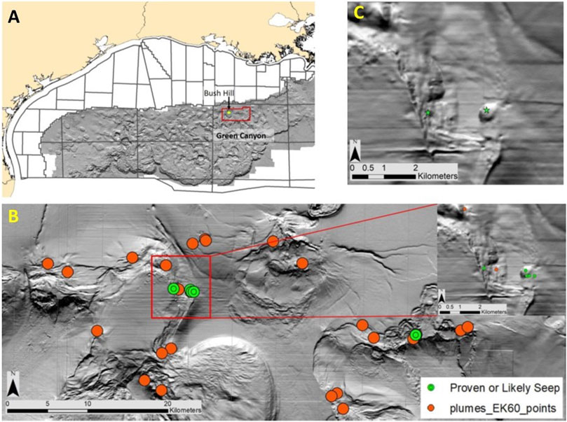
FIGURE 1. General and more detailed location maps are provided in (A–C). (A) Shows the outline of the area covered by our Bureau of Ocean Energy Management geological exploration permit in the context of the Texas-Louisiana coastline, protraction polygons, and slope bathymetry. The location of the Bush Hill mud volcano is indicated by a star. (B) Provides a detailed MBES (multibeam echo sounder) shaded map with the locations of oil-bearing dropcores and bubble plumes. There is an inset zoom of the area around Bush Hill. (C) Zoom of the Bush Hill area with stars indicating the location of the mud volcano and the seepage site on the slope to west of it.
Evidence of active seepage at the seafloor in the general study area is demonstrated through a variety of approaches. Multi-Beam Echo Sounder (MBES) surveys are typically conducted to acquire high-resolution bathymetry, but acoustic scattering off of bubble plumes, of sufficient bubble density, provides a means of locating active methane seepage (Weber et al., 2014). Oil droplets are not reliably imaged using MBES and so direct detection of seafloor oil seepage locations is commonly done via detection in sediments using drop cores or direct observation. The area surrounding Bush Hill has numerous seepage points (De Beukelaer, 2003; Figure 1B). The distribution of oil seepage (invariably associated with methane release) can also be assessed somewhat indirectly by examining oil slicks on the sea surface that are sourced from natural seeps.
The Bush Hill area is located below locations of persistent oil slicks imaged using Synthetic Aperture Radar (SAR) satellite imagery. The persistent nature of the seepage is demonstrated by the repeat observations (e.g., De Beukelaer, 2003). This relatively continuous seepage was one of the critical criteria for the experiment site selection. The SAR images also help to identify nearby discrete seepage points separated from Bush Hill by at least 750 m.
Bush Hill was one of the first submarine hydrocarbon seeps located on a continental slope to receive significant research attention (Brooks et al., 1984; Brooks et al., 1985; Brooks et al., 1986; Kennicutt et al., 1988b). Aspects of the Bush Hill setting that have received attention include: the hydrate deposits (Brooks et al., 1984; MacDonald et al., 1994; Sassen et al., 1998; Sassen et al., 1999; Vardaro et al., 2005; Kastner and MacDonald, 2006), the benthic chemosynthetic community (Kennicutt et al., 1988a; Brooks et al., 1989; MacDonald et al., 1989; Sager, 2002), and as a potential source of atmospheric methane (Solomon et al., 2009; MacDonald, 2011; Hu et al., 2012).
A detailed seafloor study was conducted prior to construction of the Jolliet Platform to the west of Bush Hill in GC184. The study found numerous areas of near seafloor carbonates, gas escape features, and hydrates (Kennicutt et al., 1988a). The mapping suggests that in addition to Bush Hill, some seepage has taken place over a considerable fraction of the area with one locus in the northern part of GC184 and another that is elongated N-S at the boundary between GC184 and GC185. To understand the source of hydrocarbons in the water it is therefore important to understand what parts of this general area actively seep significant volumes of hydrocarbons and which are relic, dormant, or low flux seepages. As an example we consider the potential seepage point ∼1 km west of Bush Hill.
Side-scan sonar images of the Bush Hill area collected in 2001 (De Beukelaer et al., 2003) showed two bubble plumes, one originating from the crest of the mud volcano and the other from a point on the slope to the west. The plume to the west, located near a drop core hit (Figure 1C), was not observed a year later. The western bubble plume’s location corresponds to an area with hydrate material at or near the seafloor and possible carbonates at the seafloor (Kennicutt et al., 1988b). The absence of a persistent bubble plume over the western area and the lack of surface slicks originating from that area in either 2001 or 2002 suggest that it has a lower average flux than Bush Hill and/or is only periodically active.
Aside from that just discussed, no bubble plumes have been imaged within >3 km of Bush Hill suggesting that any ongoing hydrocarbon seepage is relatively intermittent, low volume or dispersed. In situ analysis of dispersed flow at Bush Hill indicates that most venting is focused (Kastner and MacDonald, 2006). Measurements of background fluid fluxes reveal both up-flow and down-flow on the crest of the mud volcano (Tryon and Brown, 2004; Kastner and MacDonald, 2006). Although flow rates approaching 2 cm/day were measured in some locations for short durations, typical flow rates are less than 0.01 cm/day with some of the pore fluids escaping the seafloor being rich in dissolved methane. This average dispersed flow is insufficient to impact in situ measurements made greater than a few centimeters above the seafloor.
The current study provides a time-integrated 3D characterization of the dissolved methane distribution around Bush Hill. We present the result of two surveys that used in situ measurements to provide two separate and relatively complete snapshots of the dissolved methane plume around the seep. The inclusion of contemporaneous current data for one of the studies provides insight into how the methane is advected from the source. Together, these two studies provide a first attempt to understand the distribution of dissolved methane around an isolated natural source.
Materials and Methods
This work is based on two field studies conducted in the spring and fall of 2018. Autonomous underwater gliders were used for in situ analyses in both studies. Uncertainty about the extent and concentration of dissolved methane around Bush Hill and the nature of the near-bottom currents led us to deploy two distinct sampling strategies in the spring and fall. Time constraints did not permit us to modify the fall instrumentation packages based on the results of the spring study. We therefore opted for slightly different configurations of hardware as part of the experiment design. The spring results did provide insights that benefitted the operational execution of the fall study.
In the spring experiment, three Teledyne Slocum gliders were operated by Blue Ocean Monitoring (Australia). They were equipped with hybrid thrusters allowing them to travel at near constant elevation above the seafloor. The fall experiments used two Alseamar SeaExplorer gliders operated by Alseamar (France). The SeaExplorers relied solely on their buoyancy drive for thrust. They traverse the water column in “yos” that consist of a dive from a known position to near the bottom and then an ascent to the surface to reposition. They collected near bottom data using low amplitude mini-yos that generally kept the vehicle within ∼25 m of the seafloor.
The sensor hardware used for the studies had two key differences. In the fall study Alseamar included a downward-looking ADCP on one of the two gliders. This provided collocated current and chemical measurements. The other major difference is that the sensitivities of the Franatech METS methane sensors differed with the spring study using ultra-high sensitivity and the fall using just high sensitivity sensors.
In the spring experiment the ultra-high sensitivity METS provided detection limits ∼1 nM and non-linear performance at greater than 500 nM. The fall experiments used the high sensitivity METS with detection limit of ∼20 nM and non-linear performance at greater than 1,000 nM. These are the theoretical quantitation limits, in practice the exact calibrations differ so an offset from the lower limit was defined to serve as a quantitation limit. For the data collected in the spring, with the more sensitive detectors, a conservative estimate of 10 times the environmental background is used for the quantitation limit (25 nM). Data from the fall experiments was corrected for a systematic baseline response difference and adjusted to two times the detection limit to yield quantitation values of 40 nM (glider SEA023) and 60 nM (glider SEA027).
The average sampling time frequency for the METS used in the spring study is every ∼1 s. The fall survey METS sampled every ∼1.5 s. The average horizontal speed of the gliders in the spring study was ∼2.5 m/s and the in the fall study their horizontal speed was ∼1.75 m/s. These combinations of sampling frequency and horizontal speed give similar lateral sampling of ∼2.5 m for the spring study and ∼2.6 m for the fall.
The capabilities of the METS senors were essential to this study. The high sensitivity allowed methane detection to background levels to define the extent of the methane plume. The in situ measurements provided extremely high spatial resolution and were reported from the gliders in near real time (allowing on-the-fly adjustments to operational plans). In total, more than 2 million near-bottom methane analyses were collected over Bush Hill during the spring and fall studies. The high density of data allows a much more confident understanding of the spatial and temporal characteristics of the methane distribution in the near and mid-field at Bush Hill.
A limitation of the METS sensor is its ability to provide a strictly quantitative methane determination because of its relatively significant uptake and washout delays. The T90 time of a sensor is the time required for it to register a concentration equivalent to 90% of the actual concentration present, reported as 1–30 min by Franatech for the METS. For example, if a clean sensor is exposed to a flow of solution with a methane concentration of 100 nM, the T90 time would correspond to how long it would take for the sensor to report a concentration of 90 nM. The greater the concentration difference of a new solution from that currently observed by the sensor the longer the T90 time. The delay associated with diffusion through the membrane and sorptive processes on the detector’s semiconductor surface, both of which scale with the magnitude of the change, are responsible for a delay in sensor response. Both processes initially take place faster with high concentration gradients in the water and slow as the concentration gradients are minimized. This means that the METS will respond quickly to significant concentration changes but in a semi-quantitative way. The limited range of temperatures encountered near the seafloor (<1.5°C) and the limited impact of the pressure range on the detector window (from ∼450 to 650 m depth) mean that the diffusion rates are essentially fixed throughout the study area. Hence the response performance of the sensor does not vary appreciably within the bounds of the study area.
Because of the signal delay inherent to the METS, the methane concentrations reported should be thought of as a kind of moving average. They are not strictly comparable to, for example, discrete seawater samples captured and analyzed in a lab. It is virtually certain that the T90 time for the sensor is never achieved because the glider is moving, the water is moving, and the methane concentration field is heterogeneous. This means the highest concentrations reported are lower than what the glider actually encountered and there is some degree of smoothing of both high and low concentration heterogeneities. However, understanding how the METS performs allowed us to interpret the data so as to generate appropriate concentration maps. The fact that the METS responds quickly to significant concentration gradients means that areas with limited concentration variations can be identified as can sharp concentration boundaries.
The best way to understand the data provided by the METS is to look at examples of data collected in different settings at Bush Hill (Figure 2). The figures shows the response characteristic of the METS associated with: moving into the plume (Figure 2A), moving inside the plume through a low concentration part (Figure 2B), moving through a high concentration area (Figure 2C), and leaving the methane plume (Figure 2D). Between dives the gliders spend 30 min or more at the surface reporting data. This assures that the METS detector has been cleared of methane to the background concentration. Therefore, during the descent, the upper limit of the methane plume can be readily identified (Figure 2A). During the early uptake of significantly higher methane concentrations, we observe a continuous and smooth point-to-point monotonically increasing signal in the highly resolved time series from the METS. When the glider is inside the methane plume in an area without abrupt concentration changes (Figure 2B), the short-term signal includes more variability on a point-to-point basis (i.e., contrast the monotonically increasing uptake data and the line defined by the plateau data that includes numerous increases and decreases about the mean trend). When the glider is traversing parts of the plume with relatively high methane concentrations, the same variability on a point-to-point basis is seen as at low concentrations (Figure 2C). When the gliders begin their ascent to the surface from the methane plume they quickly transit into background methane concentrations and this generates the signal characteristic seen during the initial uptake except with a monotonic decrease (Figure 2D). By analyzing the METS data at fine temporal resolution and recognizing the signal characteristics of larger concentration contrasts, we are able to more clearly distinguish the structure and boundaries of the methane plume.
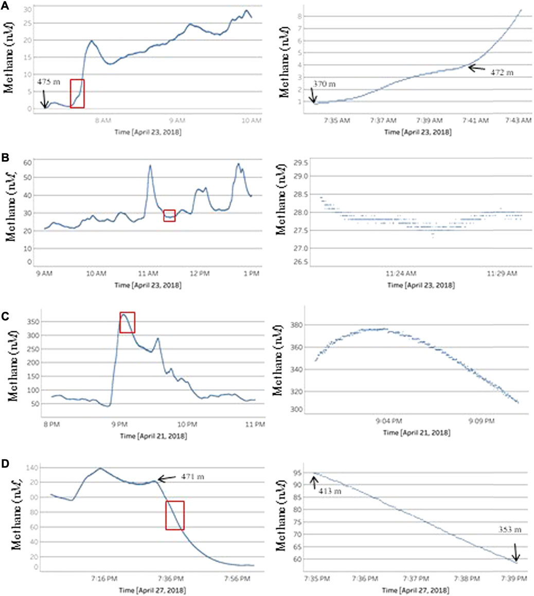
FIGURE 2. Plots of methane-data time series for glider 187 resolved at hour and minute scales (sampling frequency is 1 Hz). For each longer period time series, an inset box shows the interval presented at the minute time scale on the right side. Key water depths are noted on the plots for descending part (A) and ascending part (D) paths. Water depth for traverse paths are near constant at ∼475 m part (B) and ∼550 m part (C).
Current-velocity data were collected using a Nortek AD2CP Acoustic Doppler Current Profiler (ADCP) on every dive conducted by glider SEA027. SEA027 collected data from November 6th to the 11th inclusive but was damaged in a shark attack and no data were collected for the remainder of the survey (the glider was recovered). The ADCP data was processed in two ways depending on whether the ADCP detected the bottom. When the ADCP detected the bottom, the glider’s motion was directly resolved and high temporal and spatial resolution data was collected (on the order of 10 s and 2 m). When the ADCP could not detect the bottom, the data were averaged over a much longer duration to compensate for the differential movement between the glider and the water. All raw ADCP data was processed by the equipment provider (Alseamar).
Results
Methane Concentrations
The methane concentration provided by the METS are not strictly quantitative but are rather the smoothed values as described in the methods section. However, hereafter we discuss the measured methane concentrations as though the numerical values represent the actual concentrations present. This is done simply to reduce the number of qualifiers scattered throughout the text. We have examined all the data at high temporal resolution so that in all instances where we have found high contrasts in concentration values we can interpret their significance taking into account uptake and washout issues. We also note that while the maximum concentrations reported are assuredly lower than the maximum concentrations encountered, they are inferred to be lower by only ∼30% based on the detailed time-series analysis.
Methane concentrations measured in the spring study found maximum methane concentrations of ∼400 nM but most peak values were less than 200 nM (Figure 3). There is a systematic increase in the average concentrations measured as the study progressed. This is not interpreted to be related to an increase in flux from the seep, but rather simply reflects the progression of mapping from far to near with respect to the source. The gap in data centered on April 25th is an artifact related to bad weather and a shipboard equipment failure that required a return to port that resulted in a ∼48 h gap in data collection.
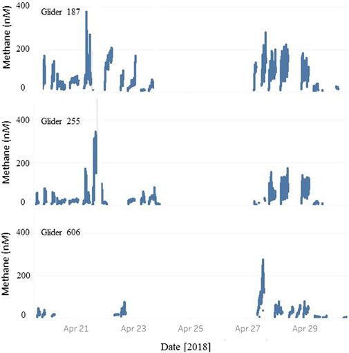
FIGURE 3. Methane concentrations measured by each glider (187, 255, 606) during the spring study. Data has been filtered to eliminate measurements taken above 450 m below the sea surface.
On average, glider 187 measured higher concentrations than the other two gliders. Glider 606 was routinely flown at a higher elevation from the seafloor and so its measurements are not directly comparable with those of 187. Comparison of measurements of gliders 187 and 255 collected within 2–3 h of each other from the same location are consistent with the METS on glider 187 reporting higher methane concentrations. However, there is significant overlap in the concentrations measured by both gliders. So while we interpret glider 187 to have reported methane values ∼10–25 nM higher than glider 255, no systematic correction could be applied.
Methane concentrations measured in the fall study found maximum methane concentrations of ∼300 nM but most were less than 100 nM (Figure 4). As with the spring study, the higher average concentrations measured later in the study are related to more traverses closer to the seep source. The low concentration measurements at the start of both gliders’ records and on the November 10th for SEA027 and the 11th for SEA023 are data collected well away from Bush Hill (and any other hydrocarbon seepage sources) and are intended to measure background concentrations.
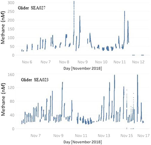
FIGURE 4. Methane concentrations measured by gliders SEA023 and SEA027 during the fall study. Data has been filtered to eliminate measurements taken above 450 m below the sea surface.
SEA027 measured four instances of methane concentrations at or above 200 nM in contrast to SEA023 which did not measure concentrations higher than 160 nM. Aside from these four high concentration dives, comparison of the remainder of the measurements from both gliders shows them to be comparable so we interpret the sensors to be consistently calibrated.
Segregating out far-field analyses from both studies, we find that the spring study found higher average concentrations relative to the fall study. Average concentrations measured in the spring were 109 (±38 at 1 SD) nM and those from the fall ∼72 (±23 at 1 SD) nM. This difference could be explained by the different METS sensitivities used, although these concentrations are well within the detection range of both. The difference could also be explained by a 35% decrease in the methane flux from the spring to fall or by more effective removal of methane from the area by advection. That the lower average concentrations in the fall correspond with lower maximum concentrations is more consistent with a decrease in net flux.
Mapping of Methane Concentrations
Combining data from the two surveys along with the current observations allow the methane concentrations surrounding Bush Hill to be analyzed spatially, temporally, and in the context of the current directions. The simplest analysis is done by integrating the data from both field studies to constrain vertical variations and projecting them to a map view for lateral variations - discounting temporal variations in both cases. This analysis is perhaps the most useful approach for understanding how far away from the source methane concentrations are elevated above background. Localized temporal variations in methane concentrations can be examined by limiting analysis to locations that were revisited two or more times within a restricted amount of time. This approach has been applied to both field studies with a time restriction of 12 h. The impact of local variations in the near bottom currents on methane concentrations is assessed by examining the data from the fall deployment from the glider equipped with the ADCP (SEA027).
The aggregate methane measurements provide a sense of the vertical and lateral extent of the integrated methane plume. The data from the two studies are integrated using concentration distributions from both studies to define volumes appropriate for averaging and deriving average values from the spring study. The upper boundary for reliable methane detection around Bush Hill can be assessed looking at detection during glider descents, when no washout concerns exist. For the spring field study, the gliders operated using thrusters and so maintained a relatively constant height off the seafloor (aided by active bottom detection) and therefore made relatively few dives. In contrast, the gliders used in the fall field study relied on the buoyancy drive for thrust and so were constantly changing elevation. Because the fall study included more frequent water column transits it provides a more robust test of the depth of initial methane detection around Bush Hill.
Most of the dives in the fall study did not detect methane until the glider was navigating close to the seafloor, but 14 out of 78 dives detected methane on descent with a maximum detection height of 170 m and an average height of 100 m. A limitation of the data from the fall study is that most of the descents were displaced from the methane source. To further examine the vertical variability around the source we constructed 500 m thick smashes (orthogonal interval projections) of the data from the spring study onto N-S and E-W vertical planes centered on the mud volcano (Figure 5). The N-S smash indicates detection of methane at ∼60 m above the mud volcano (540–480 m depth) while the E-W smash reveals ∼90 m detection height (540–430 m). Both values should be taken as minimum detection heights as few or no background measurements are present above the mud volcano. Data from the constant elevation glider traverses (spring study) are therefore consistent with detectable methane concentrations being mostly restricted to less than ∼100 m from the seafloor (with localized exceptions). In contrast, a significant number of background measurements can be found closer to the seafloor away from the mud volcano suggesting that the methane plume is domed above the source and thins vertically away from it and is concentrated near the seafloor.
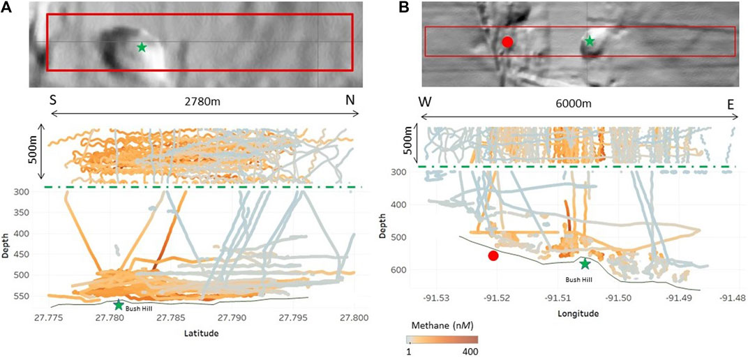
FIGURE 5. Observed methane concentrations around Bush Hill during the spring study are depicted as color shading along the paths of the gliders. The upper images are detailed gray-shaded bathymetric relief maps of the area showing location boxes for data in middle and lower images. The location of Bush Hill is marked as a green star in each and the location of another potential methane source is noted as a red circle in the E-W shaded relief map (see Figure 1C for context). The middle images shows all glider data from 300 m down used to construct the vertical section smashed to a horizontal plane. The bottom images are S-N (A) and W-E (B) 500 m thick vertical data smashes onto a plane. The projected glider paths’ color indicate the methane concentration (see scale) with orange colors indicating confident detections. The divergence of the methane scale is set at 10× the environmental background.
Using a 450 m depth cutoff for filtering data for map-view projections (∼90 m above the summit of Bush Hill) we can examine the general concentration profile away from the seepage source (Figure 6). Both studies show the highest concentrations closest to the methane source with concentrations dropping off significantly with distance. The area bounded by a radius of 500 m to the source has few non-detects and a significant number of high concentration measurements (Figure 6). For distances greater than 500 m from the source the fraction of non-detects increases significantly with increasing distance. Both studies suggest the effective radial limit of the methane plume around Bush Hill is 1,500–2,000 m.
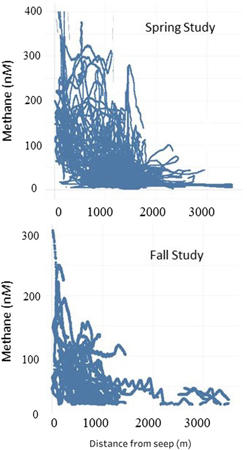
FIGURE 6. Methane concentrations from all gliders are plotted against the horizontal distance from the seep where the data was collected. The data are filtered to include only measurements below 450 m water depth. The spring study data is at the top.
Lateral variations of the methane plume are examined by projecting the data to the seafloor. Results from the spring experiment were split based on their elevation above the seafloor into 0–45 and 45–90 m (Figure 7). Both sets show high concentrations above the source with more background concentrations observed in the 45–90 m map and moving away from the source. Although limited to the south, the projected data reveal elevated methane concentrations can be detected at least 1.5 km (perhaps up to 2 km) from Bush Hill in all directions including up-slope to the west. This is consistent with the interpretation based on the vertical smashes. The data from the fall study includes, almost exclusively, data collected within 25 m of the seafloor during mini-yos (Figure 8). It shows similar spatial patterns as the spring study including lower concentrations to the east and southeast of the mud volcano summit. It is important to note that over the entire area mapped, even near the source, there is some fraction of the data that has background concentrations. This strongly suggests that the methane plume around the seep source is not continuous in space, time, or both.
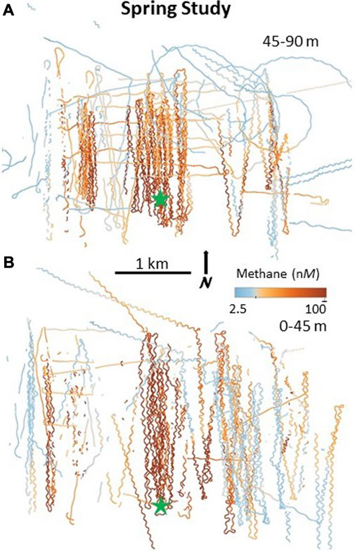
FIGURE 7. Glider traverse maps for data collected in the spring study of the Bush Hill area (green star marks seep) color coded for methane concentration. (A) shows the data binned between 45 and 90 m and (B) 0–45 m above the seafloor. The divergence in the methane color coding corresponds to the 25 nM or 10× the environmental background with orange colors indicating confident methane detection.
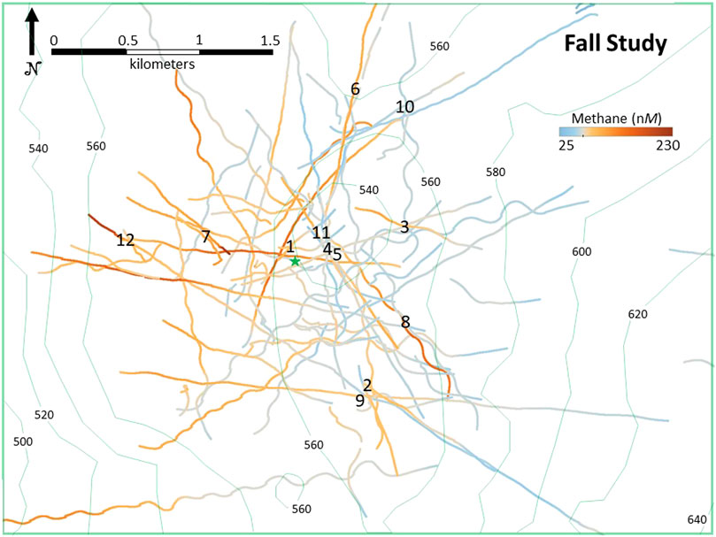
FIGURE 8. Glider traverse maps for data collected in the fall study of the Bush Hill area (green star marks seep) color coded for methane concentration. The glider paths are overlain on the seafloor bathymetry contoured in meters below sea level (bathymetry from NOAA). The divergence in the methane color coding corresponds to the quantitation limit with orange colors indicating confident methane detection. The numbers correspond to a temporal analysis (see Table 1).
Documenting temporal variability relies on multiple visits to the same site. In this regard the spring survey provided many more instances of repeat visits within a 12 h time period. Twenty five locations as close as 0.25 km and as far as 1.75 km from around Bush Hill were selected to document the extent of any temporal variations (Figure 9). Five locations closest to Bush Hill (<0.75 km) did not include any measurements below 50 nM (Figure 9). However, all of these locations show significant variations in methane concentration. Most locations more than 0.75 km distance from the seeps include at least some measurements below 50 nM and half of these include measurements below 25 nM (interpreted as the quantitation limit for the spring study).
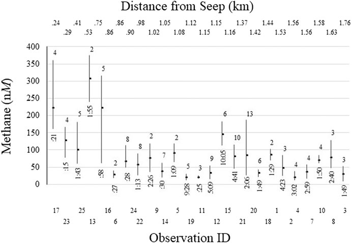
FIGURE 9. The plot shows the temporal variation at 25 points of varying distance from the source during the spring study. The horizontal distance is not scaled in the figure see the upper axis label. Observations numbers are shown on the lower axis. The number of replicate observations is shown above the observed range. The duration of observations is shown below. The vertical lines represent the spread of the observed concentrations with the tick mark indicating the average for each set of measurements.
Collectively, the temporal variability data suggest that the dispersal pattern of methane around Bush Hill is highly variable in both time and space. The areas closest to the source (∼0.75 km) appear to have concentrations that are almost always above detection limits, generally above 100 nmol, and with an average concentration of ∼160 nM (spring study, ∼100 nM for the fall study). At distances greater than ∼0.75 km the methane concentrations are typically between 50 and 100 nM (fall study ∼45–65 nM) and it is common for repeat sampling sites to include values both above and below quantitation limits. Based on the spring study concentrations, the general picture these observations generate is of an area surrounding the source (radius ∼0.75 km) with persistently higher methane concentrations (∼160 nM) but still occasionally having areas with little or no detectable methane. This central area is surrounded by a ∼concentric region that extends another ∼0.75 km and has concentrations around ∼70 nM, and with some places varying above and below the detection threshold on time scales of tens of minutes to several hours.
Current Directions and Speeds
Comparison of currents resolved into East and North vector components shows that the water column can be subdivided into three parts (Figure 10). In the upper 100 m of the water column, the currents are generally less than 0.3 m/s and are skewed to a northern direction. These results are consistent with satellite surface current models over the study area that suggest the location was centered between two counter rotating eddies. There is no systematic temporal pattern to the measured currents on the scale of days with significant ranges in both directions and speed occurring. Within-day variations could be related to diurnal forces such as tides and/or changing wind conditions during day and night.
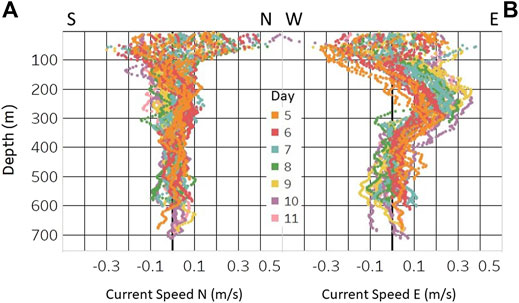
FIGURE 10. Average current data for all dives showing how the north (A) and east (B) velocity components vary with depth (vertical axis). The data are color-coded by the date of the dive (November 2018).
The depth range ∼100–400 m shows a pronounced eastward directed current with speeds ranging between 0.15 and 0.3 m/s (Figure 10). This current is most pronounced at 250 m depth. Focusing on the magnitude of the east vector component of the current reveals an increasing trend from the 5th to the 10th of November, best seen between 200 and 300 m.
For depths below 400 m, the current velocities are uniformly slower, generally less than 0.1 m/s, with no preferred orientation (Figure 10). In this depth range, there is no temporal pattern in the north-south component, but data from the 5th and 6th of November are modestly skewed to the east while results from the 9th and 10th are modestly skewed to the west.
Dives that approach within ∼25 m of the seafloor allow the ADCP to achieve bottom-lock. This extra positioning data allows processing of the ADCP data that resolves the bottom-current structure at a much higher spatial and temporal resolution. For near-bottom studies, the gliders conducted mini-yos each consisting of an approach toward the seafloor and ascent away after achieving a depth of ∼5 m from the seafloor. The bottom-water current data is analyzed initially by looking at the average current measured in each mini-yo. We then consider current variations within mini-yos that helps resolve the current structure on the scale of individual meters vertically and laterally and on time scales of 2–3 s.
Average mini-yo data shows a speed range from less than 0.03 to ∼0.18 m/s (Figure 11). The aggregate data reveal no simple relations in terms of current orientations or speeds relative to the bathymetry around Bush Hill. The data collected contain direction reversals and changes in speed that span the observed range on time scales of less than 4 h.
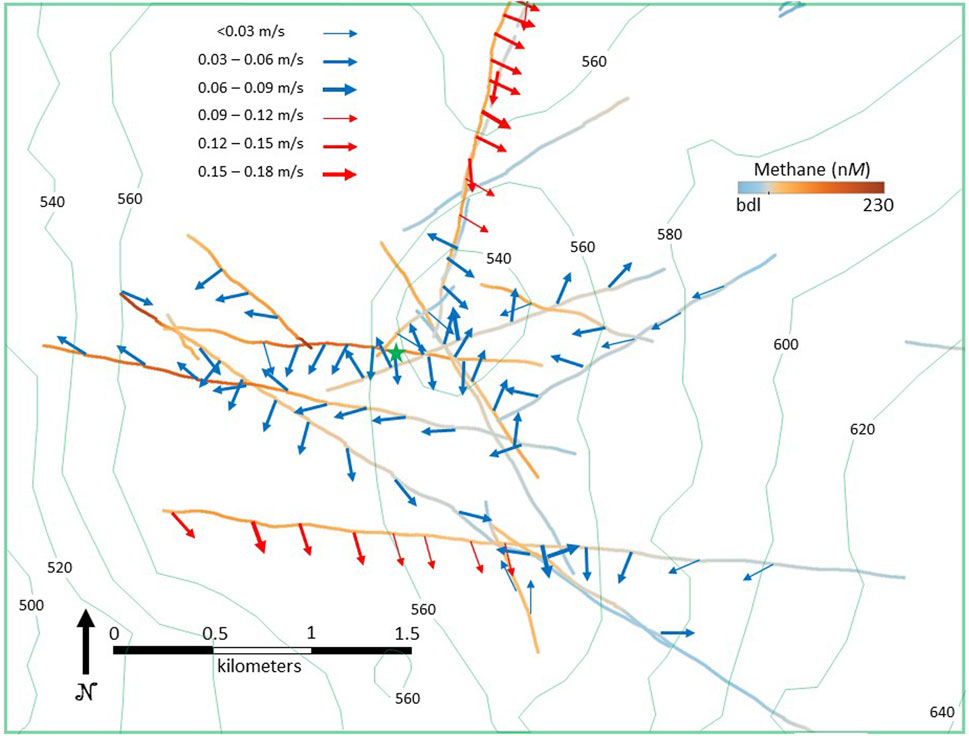
FIGURE 11. Average near-bottom current measurements are shown as vectors (see legend). Each vector tail is located on the glider path for that data point. Glider paths are color coded to indicate the methane concentration with orange colors indicating confident detection (see e.g., Figures 4–6). The green star represents the venting location for Bush Hill (27.7811°N, 91.5082°W). Bathymetry shown is in meters below sea level.
Near-bottom dives on Nov. 6th traversed relatively short distances and had a limited number of mini-yos (Figure 12). These dives found bottom-water currents with low speeds and highly variable directions. Two mini-yos on the northern crest of Bush Hill found low speed currents (less than 0.06 m/s) that nearly reversed directions over ∼3.5 h from WNW to ESE. Two dives on the southern flank of Bush Hill near the end of the Nov. 6th again found similar low current speeds and current directions that shifted by ∼90° from to the W to the N in ∼3.5 h.
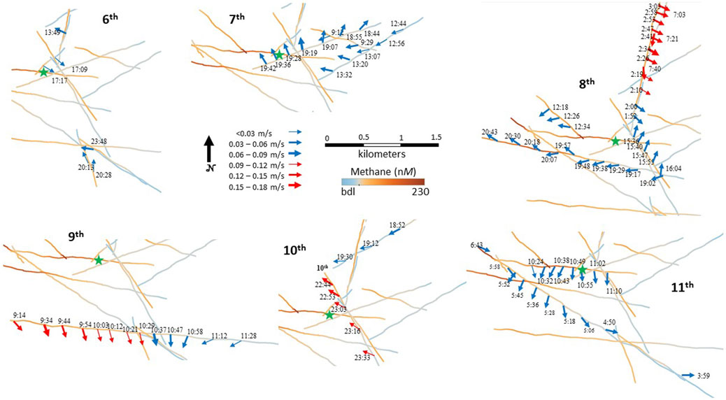
FIGURE 12. Detailed daily average near-bottom current measurements. Data as per Figure 10 but split out for each day with acquisition times indicated at the tail of each vector.
Three near-bottom dives took place on Nov. 7th skewed to the east of, and crossing just over the top of the summit of Bush Hill (Figure 12). These dives found bottom-water currents with low to intermediate speeds and variable directions. Currents measured in the earlier part of the day to east of the summit flowed up slope with low speeds (less than 0.06 m/s). A traverse over the summit later in the day found directions varying around being directed due north, without regard to the bathymetry and with higher average speeds (0.03–0.09 m/s).
Five near-bottom dives took place on November 8th crossing over the summit of Bush Hill and extending significantly far to the north and west (Figure 12). These dives found bottom-water currents with speeds ranging over nearly the entire observed range (0.03–0.18 m/s) and with directions in every quadrant. Currents measured in the earlier part of the day from ∼2:00 to 8:00 on the north side of the mud volcano found mostly high speed currents that shift from predominately eastward to southward directed over this time. Three dives later in the day (after 12:00) found a restricted range of speeds (0.03–0.06 m/s) with directions that varied from toward NNE to toward WSW.
A single near-bottom dive took place on Nov. 9th crossing from west to east over the southern extension of Bush Hill (Figure 12). This took just over 2 h and found bottom-water currents with directions predominately directed to the south but speeds ranging over the entire observed range. Current speeds were highest at the start of the dive to the west of Bush Hill (0.12–0.18 m/s) and dropped progressively as the glider went over the top of the elongate southern part of the mud volcano and traversed down the eastern slope (<0.03–0.09 m/s).
Three near-bottom dives took place on November 10th with one recording only a single mini-yo well to the east of Bush Hill and the other two traverses near/over the summit (Figure 12). Bottom-water currents were predominately to the west with a significant range of speeds (<0.03–0.15 m/s). The single average current measurement well to the east of Bush Hill, and nearly 100 m below its summit, is of a slow current (<0.03 m/s) flowing nearly due south. Similar low speed currents were measured just to the north of Bush Hill 13 h later directed to the ∼SW. However, 3 h later on a traverse over the summit of Bush Hill currents with speeds up to 0.15 m/s were measured flowing to the NW.
Two near-bottom dives took place in the first half of November 11th with one being an exceptionally long traverse from the SE across the southern flank of Bush Hill and the other traversing from nearly due west near/over the summit and directly over the seep vent (Figure 12). Bottom-water currents were slow with a limited range of speeds (<0.03–0.06 m/s) and directions ranged over only slightly more than 90° from directed E to directed SSW. A traverse from the southeastern slope to well to the west of the summit took nearly 3 h to complete documenting little variation in current speed (0.03–0.06 m/s) and directions that sweep from directed nearly E to directed SW and then abruptly back to directed SE. The change in current direction from SW to SE is found between data points separated by ∼100 m and ∼6 min between average measurements. A traverse over the summit that took 50 min documented consistent current speeds (0.03–0.06 m/s) flowing ∼S.
Analysis of the detailed current information contained in each mini-yo has the potential to reveal significant advection of methane near the seafloor. Each mini-yo resolves the 25 m above the seafloor into 2 m cubic bins. While most of the traverses did not image any significant structure to the bottom water currents, some revealed discrete higher velocity bottom water flows. Two examples of bottom water flows are shown from Nov. 8th and 9th. The traverse on the 8th starts on the lower slopes of the mud volcano on the north side and progresses away from the mud volcano up the slope to its north. The data reveal a much higher velocity flow in the bottom ∼8 m of the seawater column (Figure 13A). The traverse is oriented perpendicular to the flow direction. The higher-velocity bottom-water current has a width of ∼1 km and the southern and northern margins of the flow are elevated from the seafloor.
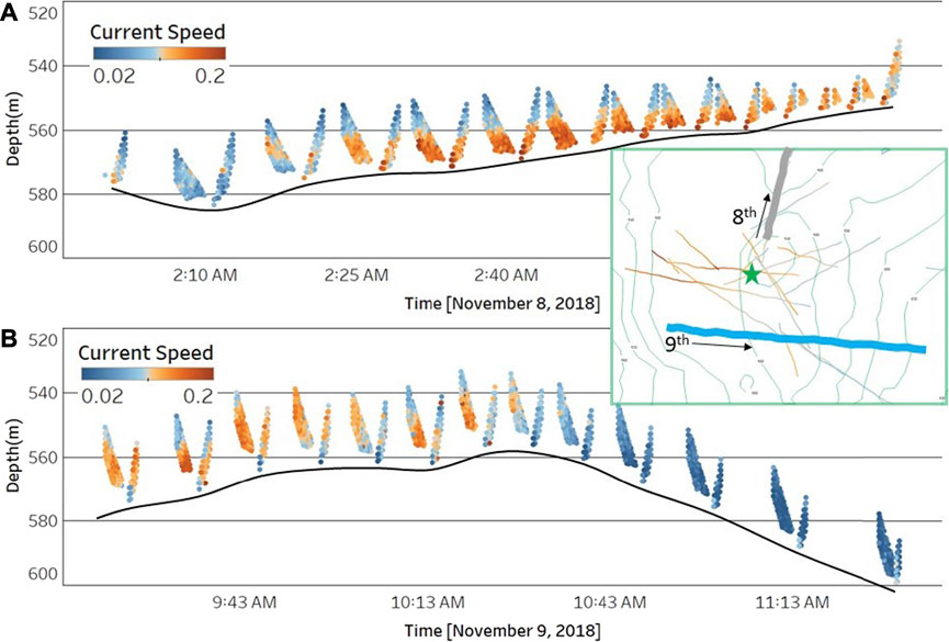
FIGURE 13. Detailed on-bottom data showing strong near bottom currents. (A) shows data for the 8th of November and (B) for the 9th. The current speeds shown range from 0.02 to 0.2 m/s and the color scale diverges at 0.11. The horizontal axes indicate time of acquisition for each day. The inset map shows the locations of the traverses relative to Bush Hill and the local bathymetry (Figure 10). The current direction of the 8th is predominately to the east and on the 9th to the south (Figure 11) so in both cases the traverse is across the flow direction. The pairs of data points are collected on the descent and ascent of each mini-yo.
The traverse on the 9th starts to the west of the mud volcano and goes up and over its elongate southern flank. The glider traverse is perpendicular to the flow direction and samples a 1.5 km wide part of the flow (truncated on the western side). This flow has a variable height, ranging from ∼6 to >14 m (Figure 13B). The higher-velocity flow is not restricted to the bottom and is decoupled from the seafloor both internally and at its eastern margin. The vertical extent of this flow is not constrained as higher velocity water is observed all the way to the top of some mini-yos.
Methane Concentrations and Current Directions
The methane plume structure at Bush Hill is potentially dictated by several processes but the most important of these that we can constrain is current variations. Short term variations in flux, for example, could lead to spatial variations in concentration but we have no constraints on it during the field studies. Therefore in the analysis below we focus on spatial and temporal variations that can be ascribed to current variations. The analysis is necessarily restricted to the fall study data as there was no ADCP deployed in the spring.
Examination of the data from the SEA027 traverses on the 6th to the 11th of November should provide direct insight into methane advection from the source (Figure 12). All current measurements on the 6th and 7th have current directions moving toward the source, or nearly tangent to it, suggesting the measurements locations are upwind of the source. Despite being upcurrent, the measurements on these days are split nearly equally between those that detected methane and those that did not. The parts of traverses closest to the source detected methane on both the 6th and 7th, but methane was also detected on the 6th in locations ∼1 km to the south despite northward directed currents. Traverses on the 8th and 9th found currents coming from the source or tangent to it, so they are mostly downcurrent of the source, and include some of the highest measured current velocities (Figure 12). Throughout most of the lengths of all these traverses methane is detected. Currents on the 10th are mostly oriented toward the source, upcurrent, with the traverse closest to the source measuring methane and the more distant traverse not detecting methane. Two traverses on the 11th include one that traveled over the source and another to the southwest that found current orientations from the source (downcurrent). Both traverses detected methane over most of their lengths except for the most distal part of the southwestern traverse.
The temporal variation of the currents can be examined by comparing repeat glider visits to a local area (less than 20 m radius) either by SEA027 (equipped with the ADCP) or where nearby ADCP at ∼the same time (within an hour) is recorded. We identified 12 times in the data where these criteria were met (Table 1). To simplify the data interpretation we characterize the current direction as above with the vector orientation described as with respect to the source as observed from the data collection point. Thus, currents can generally be flowing: from the source (observation is downcurrent), toward the source (observation is upcurrent), or tangent to the source (defined as being at approximately a right angle to the line connected the observation to the source).
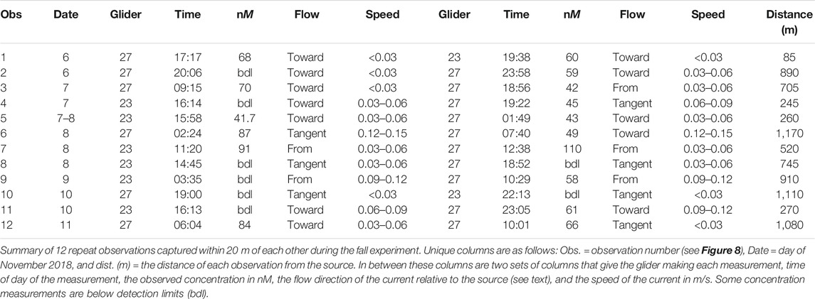
TABLE 1. Collocated observations with current data.
Two of the twelve repeat visits (7 and 9) have both observations with the current flowing from the source (Figure 12 and Table 1). Observation 7 has the two highest measured concentrations (∼100 nM) for all 24 measurement showing that high concentrations can persist locally for times of at least an hour. In contrast the first measurement at location 9 was below detection despite the current flowing from the source but ∼7 h later the concentration had increased to ∼70 nM. Two sets of observations (8 and 10) had both measurements below detection limits and in all four instances the current was tangent to the source. There are four examples of observations wherein the current was persistently flowing toward the source and these include examples of the methane concentration increasing, decreasing, and remaining the same on time scales from 2 to 7 h. There is a single example (observation 3) of the current direction reversing, initially flowing toward the source and ∼10 h later flowing from the source. In this instance the concentration decreases from 70 to 40 nM between measurements.
Discussion
Methane Distribution Around Bush Hill
Although the methane measurements and the fluid dynamics of the system indicate that it is not possible to image a static distribution of the methane concentrations around Bush Hill, a time averaged methane distribution pattern can be proposed. Toward this end we construct what we infer to be a 3D map of the time-averaged methane concentrations around Bush Hill beginning with the vertical distribution.
The descending dives place an effective ceiling for reliable methane detection over Bush Hill area at 100 m. This is consistent with prior hydrocast ex situ sampling (Solomon et al., 2009) and is typical for other ex situ sampling efforts above seeps releasing methane bubbles (e.g., Römer et al., 2019). However, the lateral glider operations in the spring study suggest that this result may reflect the methane detection height only near the source as dives more offset from the source, and lateral traverses, indicate lower maximum detection height (Figure 5). Intuitively it makes sense that ascending methane bubbles from the source would give rise to higher methane concentrations higher in the water column above the source. To uniformly define a bound for methane concentrations that are, on average, always above detection limits over the entire area we use an average detection concentration for methane of 25 nM (spring study) and require that methane be detected ∼50% of the sampling times (a 25 nM isosurface). These criteria generate a boundary over the seep that has a domed structure and extends out to ∼1,500–2,000 m.
The 25 nM isosurface surface defines a volume for the 3D map. To define concentration regions within that volume we use a combination of the map distributions for different depths (e.g., Figure 7) and smashes onto vertical planes (e.g., Figure 5). The 3D volume is not adequately sampled to robustly define lateral variations in all directions with confidence so we use a radially symmetric model. This allows us to define discrete volumes with average concentrations (Figure 14). The model honors the concentration patterns seen in both the spring and the fall but relies on the spring study for the concentrations.
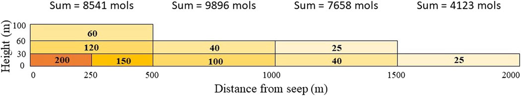
FIGURE 14. Shown is a half space block model for the concentration variations around the Bush Hill seep site. The numbers in each block indicate average concentrations in nM. The sums above the model are the total number of moles of methane contained in each 500 m wide volume assuming radial symmetry.
There are very few studies, of which we are aware, that present spatial patterns for dissolved methane around seeps. Solomon et al. (2009) studied methane release from Bush Hill with a primary focus on methane transfer to the atmosphere. As part of that work they did ex situ sampling during three submersible dives and 5 hydrocasts. The data is presented as a sparse radial cross-section of methane concentrations in the water column. Their cross section suggests methane concentrations > 1,000 nM extend more than 300 m away from Bush Hill and up to 80 m elevation within the first 150 m. Concentrations this high would have been above the linear range for the detectors used in the spring study and at or slightly above those used in the fall study. However, no concentrations were measured that approached the non-linear portions in either study. It is important to note that the near source sampling by Solomon et al. was done via submersible and intentionally sampled near the bubble streams, creating a bias toward high concentrations.
The Impact of Currents on Methane Distribution
Even slow currents will move methane released from a seep three to four orders of magnitude faster than diffusion so advective transport explains the methane distribution around Bush Hill. Prior on-bottom work at Bush Hill (Tryon and Brown, 2004; Kastner and MacDonald, 2006) has found little evidence of a distributed source for methane so it is reasonable to consider it as a point source. Taking methane as a passive chemical tracer from a point source one might be inclined to draw an analogy with smoke from a chimney. Using this analogy, the currents are expected to carry the methane downwind away from the source and thereby create an asymmetric distribution. The combined collection of current and compositional data (Figures 11, 12) allow us to test this model and find it lacking. We do observe some high concentrations downwind from the source but we also find high concentrations upwind of the source (Table 1). In general there is no clear relationship between the current direction relative to the source and the methane concentration observed.
Taking the near bottom average current data as a whole (Figure 11), there is no coherent direction in any area that persists over time. So in the analogy, the chimney is not located in a regular wind field that transports the smoke away; rather it is in an area with generally slow moving currents that change directions on time scales of hours. We suggest a better analogy is to think of the area surrounding Bush Hill as a smog basin with a central source. In this case the basin does not have any actual physical boundaries—there is higher bathymetry to the west and north but the seafloor slopes away to the east and south (Figure 1). Rather, the methane (smog) is retained around the source by the lack of any organized current to sweep it out of the area. The concentrations decrease vertically and laterally away from the source with progressive dilution.
Using a smog basin analogy, we can readily understand the lack of correlation between current and concentrations. The methane is being moved back and forth around the source so there is no particular significance to being upwind or downwind over the timescales of hours. The data from the spring and fall experiments define a similar sized detection radius – somewhat smaller in the fall. This could be an approximation of a quasi-steady-state environment around Bush Hill.
Temporal Aspects of Methane Distribution
Assuming the methane plume observed around Bush Hill is generally (always?) present, we can consider how its total methane content relates to that being released from the seep. On bottom characterization of the bubble flux from Bush Hill gives an output from the seep of ∼5,390 mol/day (Leifer and MacDonald, 2003). Summing over the entire methane plume (Figure 14) gives a total of ∼30,200 mol of methane or about 5.6 days equivalent of seeped methane. Similar calculations for the methane plume model proposed by Solomon et al. (2009) suggest 1.8 days equivalent. For the observed methane concentrations, these times are far too short to explain the marginal loss of methane via microbial oxidation (Pack et al., 2011). The upper boundary of the plume is interpreted to be controlled by more organized advective transport and dilution at higher levels in the water column (Figure 11); whereas the lateral margins simply reflect progressive dilution away from the source.
The presence of a persistent methane plume around the source could promote the stability of exposed methane hydrates (Kennicutt et al., 1988b). The initial growth of structure II or structure H hydrates (Sassen and MacDonald, 1994) at the depths of Bush Hill (>500 m) would be favored even at much higher water temperatures (at least up to 17°C) (Yin et al., 2018). In order to persist however, the exposed hydrates must maintain a methane concentration in the surrounding seawater that is at hydrate saturation—otherwise the hydrates would dissolve until the seawater was saturated. In the chimney analogy the saturated boundary layer around the hydrates would be continuously stripped away by the organized currents. In the smog basin analogy there should be a higher concentration plume of methane surrounding the hydrates so disruptions of the saturated boundary layer would not introduce “fresh” seawater but rather methane-rich seawater thereby minimizing the concentration gradient around the hydrates and reducing loses due to dissolution.
In their analyses of the hydrate dissociation Lapham et al. (2014) conclude that the observed long term stability of methane hydrates at Bush Hill is inconsistent with expected rates based on laboratory and in situ test measurements. They also conclude that the methane flux from below is insufficient to maintain the seafloor hydrates in a ∼steady state condition. They infer that the long term stability of seafloor hydrates at Bush Hill and other GoM seepages site is related to having a protective sediment cover that limits dissociation by maintaining saturation methane concentrations in pore water adjacent to the hydrate. The sediment cover is required to shield the saturated boundary layer from being depleted by currents. Our findings suggest that low current speeds and locally high methane concentrations (within a few centimeters of the hydrate) can also help promote long-term hydrate stability.
We hypothesize that the stabilization of exposed seafloor hydrates at other seep sites is indicative of the long-term presence of elevated methane concentrations and the current structure that this requires. If true, then the presence/absence of seafloor hydrates might be used as a test for grouping areas to contrast the character of their biologic communities. In particular we expect methane-oxidizing microbes in the water column to be at higher concentrations and to occupy a significantly greater volume at seeps with exposed hydrates.
Using the Observed Methane Distribution to Better Understand Seepage
The distribution of dissolved methane around the Bush Hill mud volcano is governed by the flux of methane from the seep and subsequent distribution by near-bottom currents. The data are insufficient to allow us to draw hard conclusions about details of the methane release. A simplification that is implicit to some of the preceding interpretations is that the release of methane from Bush Hill can be fairly approximated as constant over time scales of at least 10–20 min and up to 1–2 h. This simplification allows us to makes sense of the repeat current and concentration data in Table 1, for example. If the methane flux from the source dropped substantially or stopped entirely between the measurements, then the relevance of currents moving toward or away from the source relative to observation point would be far more nebulas. The fairly regular radial distribution of methane around Bush Hill would be far more complicated to explain as a product of both a varying source flux and varying current patterns. In this case the flux and currents would have to co-vary to explain the methane distribution. Thus, while a quasi-steady state flux is not strictly required by the data; we interpret the system to behave in this way as it provides the simplest explanation of the observations.
The limited amount of data on the distribution of dissolved methane at seeps means that we cannot interpret our data by analogy; i.e., there is no basis to characterize the methane plume at Bush Hill as typical or unusual. The approach we used to collect the data is relatively low cost for ocean field-work and so could be used to survey other thermogenic and biogenic sources of methane seepage to develop a more general understanding. It is our hope that others will leverage these methods to provide a more complete understanding of dissolved methane around seepage sites.
There are a number of potential changes to the experimental design that could provide more detailed and better constrained results. For example, more gliders (four or five) all equipped with ADCPs could provide an understanding of current variability in both space and time. A laser-based methane detector could provide similar sensitivity to the METS and reduce or eliminate the smoothing effect on the quantitation imparted by it. Collecting contemporaneous water samples, either from the glider(s) or via hydrocasts, could validate in situ concentration measurements.
Conclusion
We present the findings of two in situ characterization studies of methane concentrations around the Bush Hill mud volcano conducted in the spring and fall of 2018. High spatial resolution (∼5 m) mapping of methane concentrations as close as ∼5–90 m above the seafloor allowed a 3D understanding of the methane plume. Maximum observed concentrations were ∼400 nM, well below concentrations documented by ex situ samples captured via ROVs and submersibles at Bush Hill and other seep sites (which exceed 10,000 nM). On the other extreme, we found areas throughout the methane plume that had methane concentrations that were below detection limits. As might be expected, the frequency of non-detects increases away from the source. We interpret the concentration data to indicate the presence of a detectable methane plume within 30 m of the seafloor up to 2 km away from the source in all directions despite significant variations in the seafloor bathymetry.
Repeat sampling demonstrated significant variations in methane concentrations (and current directions) occur on time scales of 1–2 h. The majority (>90%) of the analyses conducted close to the source were above detection limits. At 750 m distance from the source, only about 65% of the analyses were above detection limits. This significant temporal and spatial variability presents a challenge for interpreting limited ex situ sampling. Comparison of the average results from the spring and fall studies suggests an overall decrease in the amount of methane present around the seep of ∼35%. However, nearly all other characteristics of the methane plume were similar between both studies.
By coupling the concentration data with current data we are able to demonstrate that there is no pervasive transport of methane away from the seep source (i.e., as one might picture for a classic chimney plume). The dissolved methane associated with the seepage lingers in the area of the source because the near bottom currents vary in direction often enough that they provide no effective long-distance transport. Comparison of observed total methane in the plume with estimated flux from the seep suggests that an equivalent of about 6 days accumulated methane is found in the plume. Examples of relatively high velocity (up to 0.18 m/s) near bottom currents with limited lateral extents were documented by high resolution ADCP coverage. If these currents were to persist for as long as 5 h they have the potential to displace methane located in the lower ∼20 m of the water column from the 2 km radius vicinity. Episodic occurrences of such currents may explain some of the significant temporal variations in concentration.
Data Availability Statement
The datasets presented in this article are not readily available because Data release is limited by ExxonMobil. Requests to access the datasets should be directed to d2lsbGlhbS5wLm1ldXJlckBleHhvbm1vYmlsLmNvbQ==.
Author Contributions
All authors contributed to the field effort with JB dealing with operations and planning, GS handling data ingestion and geodetic issues, and WM analyzing current and geochemical data. All three authors provided input into the ideas contained in this manuscript. WM did most of the manuscript preparation drawing heavily from internal reports to which all three authors contributed significant blocks of text and analyses. All authors provided direct input into the final versions of text and figures.
Funding
ExxonMobil’s Upstream Research Company provided all funding for the field work and subsequent data analysis.
Conflict of Interest
Authors WM, JB, and GS were employed by the company ExxonMobil Upstream Research Company during the period this research was conducted. ExxonMobil has never had working interest in GC blocks 184 and 185 (the Bush Hill area). The findings of this research have no bearing on any current development or production activities.
Publisher’s Note
All claims expressed in this article are solely those of the authors and do not necessarily represent those of their affiliated organizations, or those of the publisher, the editors and the reviewers. Any product that may be evaluated in this article, or claim that may be made by its manufacturer, is not guaranteed or endorsed by the publisher.
Acknowledgments
The field work presented here benefitted significantly from contributions from scientists associated with Alseamar especially in relation to analysis of the ADCP data and from Blue Ocean Monitoring. We also wish acknowledge significant contributions from other researchers at ExxonMobil. Lastly, we are thankful for ExxonMobil’s Upstream Research Company financial support of this effort and their interest in publishing the results.
References
Åström, E. K. L., Carroll, M. L., Ambrose, W. G., Sen, A., Silyakova, A., and Carroll, J. (2017). Methane Cold Seeps as Biological Oases in the High-Arctic Deep Sea. Limnol. Oceanogr. 63, S209–S231. doi:10.1002/lno.10732
Brooks, J. M., Cox, H. B., Bryant, W. R., Kennicutt, M. C., Mann, R. G., and McDonald, T. J. (1986). Association of Gas Hydrates and Oil Seepage in the Gulf of Mexico. Org. Geochem. 10, 221–234. doi:10.1016/0146-6380(86)90025-2
Brooks, J. M., Kennicutt, M. C., Fay, R. R., McDonald, T. J., and Sassen, R. (1984). Thermogenic Gas Hydrates in the Gulf of Mexico. Science 225, 409–411. doi:10.1126/science.225.4660.409
Brooks, J. M., Kennicutt, M. C., Macdonald, I. R., Wilkinson, D. L., Guinasso, N. L., and Bidigare, R. R. (1989). “Gulf of Mexico Hydrocarbon Seep Communities: Part IV - Description of Known Chemosynthetic Communities,” in Proceedings of the 21st Offshore Technology Conference, OTC, Houston, TX, May 1989. 5954, 663–667.
Brooks, J. M., Kennicutt, M. C., II, Bidigare, R. R., and Fay, R. R. (1985). Hydrates, Oil Seepage, and Chemosynthetic Ecosystems on the Gulf of Mexico Slope. Eos 66, 105. doi:10.1029/eo066i010p00106-01
Coleman, J. M., Roberts, H. H., and Bryant, W. R. (1991). “Late Quaternary Sedimentation,” in The Gulf of Mexico Basin, The Geology of North America. Editor A. Salvador (Boulder, CO: Geological Society of America).
Cordes, E., Hourdez, S., Predmore, B., Redding, M., and Fisher, C. (2005). Succession of Hydrocarbon Seep Communities Associated With the Long-Lived Foundation Species Lamellibrachia luymesi. Mar. Ecol. Prog. Ser. 305, 17–29. doi:10.3354/meps305017
De Beukelaer, S. M., MacDonald, I. R., Guinnasso, N. L., and Murray, J. A. (2003). Distinct Side-Scan Sonar, RADARSAT SAR, and Acoustic Profiler Signatures of Gas and Oil Seeps on the Gulf of Mexico Slope. Geo-Mar Lett. 23, 177–186. doi:10.1007/s00367-003-0139-9
De Beukelaer, S. M. (2003). Remote Sensing Analysis of Natural Oil and Gas Seeps on the Continental Slope of the Northern Gulf of Mexico. MSc thesis. Mexico: Texas A&M University, 117.
Di, P., Feng, D., Tao, J., and Chen, D. (2020). Using Time-Series Videos to Quantify Methane Bubbles Flux from Natural Cold Seeps in the South China Sea. Minerals 10 (3), 216. doi:10.3390/min10030216
Galloway, W. E., Bebout, D. G., Fisher, W. L., Dunlap, J. B. J., Cabrera-Castro, R., Lugo-Rivera, J. E., et al. (1991). The Gulf of Mexico Basin: The Geology of North America. Editor A. Salvador (Boulder, CO: Geological Society of America).
Galloway, W. E. (2008). “Depositional Evolution of the Gulf of Mexico Sedimentary Basin,” in The Sedimentary Basins of the United States and Canada: Sedimentary Basins of the World. Editor A. D. Miall (Netherlands: Elsevier), 505–549.
Girard, F., Sarrazin, J., and Olu, K. (2020). Impacts of an Eruption on Cold-Seep Microbial and Faunal Dynamics at a Mud Volcano. Front. Mar. Sci. 7. doi:10.3389/fmars.2020.00241
Greinert, J. (2008). Monitoring Temporal Variability of Bubble Release at Seeps: The Hydroacoustic Swath System GasQuant. J. Geophys. Res. 113, C07048. doi:10.1029/2007jc004704
Hu, L., Yvon-Lewis, S. A., Kessler, J. D., and MacDonald, I. R. (2012). Methane Fluxes to the Atmosphere from Deepwater Hydrocarbon Seeps in the Northern Gulf of Mexico. J. Geophys. Res. 117, C01009–C01023. doi:10.1029/2011JC007208
Hudec, M. R., Norton, I. O., Jackson, M. P. A., and Peel, F. J. (2013). Jurassic Evolution of the Gulf of Mexico Salt Basin. Bulletin 97, 1683–1710. doi:10.1306/04011312073
Johansen, C., Macelloni, L., Natter, M., Silva, M., Woosley, M., Woolsey, A., et al. (2020). Hydrocarbon Migration Pathway and Methane Budget for a Gulf of Mexico Natural Seep Site: Green Canyon 600. Earth Planet. Sci. Lett. 545, 116411. doi:10.1016/j.epsl.2020.116411
Kastner, M., and MacDonald, I. (2006). Final Technical Report on: Controls on Gas Hydrate Formation and Dissociation, Gulf of Mexico: In Situ Field Study with Laboratory Characterizations of Exposed and Buried Gas Hydrates. DOE Report (DOE Award Number: DE-FC26-02NT41328), 31.
Kennicutt, M. C., Brooks, J. M., Brooks, G. J., and Denoux, G. J. (1988b). Leakage of Deep, Reservoired Petroleum to the Near Surface on the Gulf of Mexico Continental Slope. Mar. Chem. 24, 39–59. doi:10.1016/0304-4203(88)90005-9
Kennicutt, M. C., Brooks, J. M., Bidigare, R. R., and Denoux, G. J. (1988a). Gulf of Mexico Hydrocarbon Seep Communities-I. Regional Distribution of Hydrocarbon Seepage and Associated Fauna. Deep Sea Res. 35, 1639–1651. doi:10.1016/0198-0149(88)90107-0
Lapham, L. L., Chanton, J. P., Chapman, R., and Martens, C. S. (2010). Methane Under-Saturated Fluids in Deep-Sea Sediments: Implications for Gas Hydrate Stability And Rates of Dissolution. Earth Planet. Sci. Lett. 298, 275–285. doi:10.1016/j.epsl.2010.07.016
Lapham, L. L., Wilson, R. M., MacDonald, I. R., and Chanton, J. P. (2014). Gas Hydrate Dissolution Rates Quantified With Laboratory and Seafloor Experiments. Geochim. Cosmochim. Acta 125, 492–503. doi:10.1016/j.gca.2013.10.030
Leifer, I. (2019). A Synthesis Review of Emissions and Fates for the Coal Oil Point Marine Hydrocarbon Seep Field and California Marine Seepage. Geofluids 2019, 4724587. doi:10.1155/2019/4724587
Leifer, I. (2010). Characteristics and Scaling of Bubble Plumes from Marine Hydrocarbon Seepage in the Coal Oil Point Seep Field. J. Geophys. Res. 115, C11014. doi:10.1029/2009jc005844
Leifer, I., and MacDonald, I. (2003). Dynamics of the Gas Flux from Shallow Gas Hydrate Deposits: Interaction Between Oily Hydrate Bubbles and the Oceanic Environment. Earth Plant Sci. Lett. 210, 411–424.
Levin, L. (2005). “Ecology of Cold Seep Sediments: Interactions of Fauna With Flow, Chemistry and Microbes,” in Oceanography and Marine Biology: Annual Review. Editors R. N. Gibson, R. J. A. Atkinson, and J. D. M. Gordon (Milton Park: Taylor & Francis), 1–46. doi:10.1201/9781420037449.ch1
MacDonald, I. R., Boland, G. S., Baker, J. S., Brooks, J. M., Kennicutt, M. C., and Bidigare, R. R. (1989). Gulf of Mexico Hydrocarbon Seep Communities. Mar. Biol. 101, 235–247. doi:10.1007/bf00391463
MacDonald, I. R., Guinasso, Jr., N. L., Sassen, R., Brooks, J. M., Lee, L., and Scott, K. T. (1994). Gas Hydrate that Breaches the Sea Floor on the Continental Slope of the Gulf of Mexico. Geology 22, 699–702. doi:10.1130/0091-7613(1994)022<0699:ghtbts>2.3.co;2
MacDonald, I. R. (2011). Remote Sensing and Sea-Truth Measurements of Methane Flux to the Atmosphere (HYFLUX Project). DOE Award No.: DE-NT0005638 Final Report. 164.
Pack, M. A., Heintz, M. B., Reeburgh, W. S., Trumbore, S. E., Valentine, D. L., Xu, X., et al. (2011). A Method for Measuring Methane Oxidation Rates Using Lowlevels of 14C-Labeled Methane and Accelerator Mass Spectrometry. Limnol. Oceanogr. Methods 9, 245–260. doi:10.4319/lom.2011.9.245
Peel, F. J., Travis, C. J., and Hossack, J. R. (1995). “Genetic Structural Provinces and Salt Tectonics of the Cenozoic Offshore U.S. Gulf of Mexico,” in Salt Tectonics: A Global Perspective. Editors Jackson, M. P., Roberts, D. G., and Snelson, S., 65, 153–175. doi:10.1306/m65604c7
Razaz, M., Di Iorio, D., Wang, B., Daneshgar Asl, S., and Thurnherr, A. M. (2020). Variability of a Natural Hydrocarbon Seep and its Connection to the Ocean Surface. Sci. Rep. 10, 12654. doi:10.1038/s41598-020-68807-4
Römer, M., Hsu, C.-W., Loher, M., MacDonald, I. R., dos Santos Ferreira, C., Pape, T., et al. (2019). Amount and Fate of Gas and Oil Discharged at 3400 m Water Depth from a Natural Seep Site in the Southern Gulf of Mexico. Front. Mar. Sci. 6, 700. doi:10.3389/fmars.2019.00700
Sager, W. W. (2002). “Geophysical Detection and Characterization of Chemosynthetic Organism Sites,” in Stability and Change in Gulf of Mexico Chemosynthetic Communities. Editor I. R. MacDonald (New Orleans, LA: U.S. Department of the Interior), 456.
Salvador, A. (1991). “Triassic-Jurassic,” in The Gulf of Mexico Basin: The Geology of North America. Editor A. Salvador (Boulder, CO: Geological Society of America).
Sassen, R., Joye, S., Sweet, S. T., deFreitas, D. A., Milkov, A. V., and MacDonald, I. R. (1999). Thermogenic Gas Hydrates and Hydrocarbon Gases in Complex Chemosynthetic Communities, Gulf of Mexico Continental Slope. Org. Geochem. 30, 485–497. doi:10.1016/s0146-6380(99)00050-9
Sassen, R., and MacDonald, I. R. (1994). Evidence of Structure H Hydrate, Gulf of Mexico Continental Slope. Org. Geochem. 22, 1029–1032. doi:10.1016/0146-6380(94)90036-1
Sassen, R., MacDonald, I. R., Guinasso, N. L., Joye, S., Requejo, A. G., Sweet, S. T., et al. (1998). Bacterial Methane Oxidation in Sea-Floor Gas Hydrate: Significance to Life in Extreme Environments. Geology 26, 851–854. doi:10.1130/0091-7613(1998)026<0851:bmoisf>2.3.co;2
Sibuet, M., and Olu, K. (1998). Biogeography, Biodiversity and Fluid Dependence of Deep-Sea Cold-Seep Communities at Active and Passive Margins. Deep Sea Res. Part Topical Stud. Oceanogr. 45, 517–567. doi:10.1016/S0967-0645(97)00074-X
Sibuet, M., and Roy, K. O.-L. (2002). “Cold Seep Communities on Continental Margins: Structure and Quantitative Distribution Relative to Geological and Fluid Venting Patterns,” in Ocean Margin Systems. Editors G. Wefer, D. Billett, D. Hebbeln, B. B. Jørgensen, M. Schlüter, and T. C. E. van Weering (Berlin: Springer), 235–251. doi:10.1007/978-3-662-05127-6_15
Smith, A. J., Flemings, P. B., and Fulton, P. M. (2014). Hydrocarbon Flux from Natural Deepwater Gulf of Mexico Vents. Earth Planet. Sci. Lett. 395, 241–253. doi:10.1016/j.epsl.2014.03.055
Sohl, N. F., Martínez, E. R., Salmerón-Ureña, P., and Soto-Jaramillo, F. (1991). “Upper Cretaceous,” in The Gulf of Mexico Basin: The Geology of North America. Editor A. Salvador (Boulder, CO: Geological Society of America).
Solomon, E. A., Kastner, M., MacDonald, I. R., and Leifer, I. (2009). Considerable Methane Fluxes to the Atmosphere from Hydrocarbon Seeps in the Gulf of Mexico. Nat. Geosci. 2, 561–565. doi:10.1038/ngeo574
Thomanek, K., Zielinski, O., Sahling, H., and Bohrmann, G. (2010). Automated Gas Bubble Imaging at Sea Floor - A New Method of In Situ Gas Flux Quantification. Ocean Sci. 6, 549–562. doi:10.5194/os-6-549-2010
Tryon, M. D., and Brown, K. M. (2004). Fluid and Chemical Cycling at Bush Hill: Implications for Gas- and Hydrate-Rich Environments. Geochem. Geophys. Geosyst. 5, a, n. doi:10.1029/2004GC000778
Uhlig, C., Kirkpatrick, J. B., D'Hondt, S., and Loose, B. (2018). Methane-Oxidizing Seawater Microbial Communities from an Arctic Shelf. Biogeosciences 15, 3311–3329. doi:10.5194/bg-15-3311-2018
Vardaro, M. F., MacDonald, I. R., Bender, L. C., and Guinasso, N. L. (2005). Dynamic Processes Observed at a Gas Hydrate Outcropping on the Continental Slope of the Gulf of Mexico. Geo. Mar. Lett. 26, 6–15. doi:10.1007/s00367-005-0010-2
Weber, T. C., Mayer, L., Jerram, K., Beaudoin, J., Rzhanov, Y., and Lovalvo, D. (2014). Acoustic Estimates of Methane Gas Flux from the Seabed in a 6000 km2 Region in the Northern Gulf of Mexico. Geochem. Geophys. Geosyst. 15, 1911–1925. doi:10.1002/2014GC005271
Keywords: seep, methane, Bush Hill, in situ detection, volume mapping, ocean currents, near seafloor, temporal variation
Citation: Meurer WP, Blum J and Shipman G (2021) Volumetric Mapping of Methane Concentrations at the Bush Hill Hydrocarbon Seep, Gulf of Mexico. Front. Earth Sci. 9:604930. doi: 10.3389/feart.2021.604930
Received: 11 September 2020; Accepted: 12 August 2021;
Published: 27 August 2021.
Edited by:
Ira Leifer, Bubbleology Research Intnl, United StatesReviewed by:
Jeemin Rhim, Dartmouth College, United StatesVitor Hugo Magalhaes, Portuguese Institute for Sea and Atmosphere (IPMA), Portugal
Dong Feng, Shanghai Ocean University, China
Copyright © 2021 Meurer, Blum and Shipman. This is an open-access article distributed under the terms of the Creative Commons Attribution License (CC BY). The use, distribution or reproduction in other forums is permitted, provided the original author(s) and the copyright owner(s) are credited and that the original publication in this journal is cited, in accordance with accepted academic practice. No use, distribution or reproduction is permitted which does not comply with these terms.
*Correspondence: William P. Meurer, d2lsbGlhbS5wLm1ldXJlckBleHhvbm1vYmlsLmNvbQ==