
95% of researchers rate our articles as excellent or good
Learn more about the work of our research integrity team to safeguard the quality of each article we publish.
Find out more
ORIGINAL RESEARCH article
Front. Earth Sci. , 11 May 2021
Sec. Environmental Informatics and Remote Sensing
Volume 9 - 2021 | https://doi.org/10.3389/feart.2021.601019
This article is part of the Research Topic Recent Advances in Natural Methane Seep and Gas Hydrate Systems View all 14 articles
 Peter Vrolijk1,2*
 Lori Summa1,3
 Benjamin Ayton1,4
 Paraskevi Nomikou5
 Andre Hüpers6Frank Kinnaman7Sean Sylva1
 David Valentine7
 Richard Camilli1
Natural seeps occur at the seafloor as loci of fluid flow where the flux of chemical compounds into the ocean supports unique biologic communities and provides access to proxy samples of deep subsurface processes. Cold seeps accomplish this with minimal heat flux. While individual expertize is applied to locate seeps, such knowledge is nowhere consolidated in the literature, nor are there explicit approaches for identifying specific seep types to address discrete scientific questions. Moreover, autonomous exploration for seeps lacks any clear framework for efficient seep identification and classification. To address these shortcomings, we developed a Ladder of Seeps applied within new decision-assistance algorithms (Spock) to assist in seep exploration on the Costa Rica margin during the R/V Falkor 181210 cruise in December, 2018. This Ladder of Seeps [derived from analogous astrobiology criteria proposed by Neveu et al. (2018)] was used to help guide human and computer decision processes for ROV mission planning. The Ladder of Seeps provides a methodical query structure to identify what information is required to confirm a seep either: 1) supports seafloor life under extreme conditions, 2) supports that community with active seepage (possible fluid sample), or 3) taps fluids that reflect deep, subsurface geologic processes, but the top rung may be modified to address other scientific questions. Moreover, this framework allows us to identify higher likelihood seep targets based on existing incomplete or easily acquired data, including MBES (Multi-beam echo sounder) water column data. The Ladder of Seeps framework is based on information about the instruments used to collect seep information (e.g., are seeps detectable by the instrument with little chance of false positives?) and contextual criteria about the environment in which the data are collected (e.g., temporal variability of seep flux). Finally, the assembled data are considered in light of a Last-Resort interpretation, which is only satisfied once all other plausible data interpretations are excluded by observation. When coupled with decision-making algorithms that incorporate expert opinion with data acquired during the Costa Rica experiment, the Ladder of Seeps proved useful for identifying seeps with deep-sourced fluids, as evidenced by results of geochemistry analyses performed following the expedition.
Seeps occur throughout the world along active and passive continental margins (e.g., Campbell et al., 2002), but their occurrence is rare and their distribution uneven. Comprehensive surveys do exist (e.g., Judd and Hovland, 2009; Skarke et al., 2014; Weber et al., 2014) but even they cover only a small fraction of the world’s oceans. A complete description of Earth’s cold seeps and their variability has yet to be attempted.
Seeps have been studied for decades as an important window into subsurface fluid processes. They occur in a range of geologic settings and exhibit a variety of fluid expulsion mechanisms that emanate from fluid sources 10 s to 1000 s of meters below the seafloor (e.g. Suess, 2018). They display a broad range of morphological characteristics at the seafloor, including convex, mound-shaped features associated with seep-related carbonates, concave pockmarks or collapse features, and mud volcanoes, ranging from less than a meter to several kilometers in diameter (e.g. Judd and Hovland, 2009). Different types of seeps support unique ecological niches (e.g., Sibuet and Olu, 1998; Sahling et al., 2003; Levin, 2005), allow scientists to track the release of greenhouse gases (e.g., methane and to a lesser extent carbon dioxide) from the Earth into the ocean/atmosphere (Judd, 2004; Leifer et al., 2006), and provide locations where deep-sourced fluids are sampled and analyzed (Kastner et al., 1991; Barnes et al., 2010). In this paper we emphasize the search for seeps that reflect a fluid migration pathway for fluids that may be affected by fluid-rock interactions at the subduction zone plate interface. Information about mineral reactions and corresponding fluid-rock interactions at the plate interface is useful for understanding earthquake and seismogenic processes (Peacock, 1990; Moore and Vrolijk, 1992), but the proposed methods apply to problems as far-reaching as ocean exploration on outer solar system worlds (e.g., Hand and German, 2018).
The search for seeps with deep-sourced fluids is challenging. Large areas of the seafloor must be surveyed at significant expense, yielding incomplete information (e.g. Judd and Hovland, 2009; Skarke et al., 2014; Weber et al., 2014). Geophysical tools used for the surveys are evolving rapidly, and as such, may have variable acquisition and processing approaches (e.g. Mitchell et al., 2018). Once seeps are found, sample collection and return programs for seep analysis are technologically difficult, expensive, and time-consuming (e.g., IODP scientific ocean drilling), similar to space exploration analogs (e.g. Perserverence and OSIRIS REx). To help address these issues, a flexible method is required that allows for the use of tools available on any particular day and the specific scientific objectives of the research. The optimal tools and datasets for one expedition may differ from those used on another.
To develop this methodology, we posed the problem of identifying seeps with deep-sourced fluids on the Costa Rica accretionary prism using limited, preliminary data collected above the seafloor. The methodology applied serves as a tool to assist scientists in the decision-making process for finding seeps in an objective and reproducible manner. Our approach is intended to improve the success of drilling programs, for example, and can be extended to alternative scientific objectives, like the discovery and characterization of subsea chemolithoautotrophic oases, oases with specific organisms (e.g., microbial mats), or comprehensive seep flux syntheses. Moreover, this methodology can be used in concert with autonomous vehicles that require a cognitive basis to recognize and identify potential targets and make autonomous decisions to deviate from a programmed path, linger at a site, and collect additional information to evaluate more fully.
Our approach comprises two crucial elements: a Ladder of Seeps and a Spock decision-assistance algorithm. The Ladder of Seeps is a rigorous framework of measurements and observations that make ship-based investigations more efficient and successful and guide autonomous vehicle exploration. In this study, the Ladder of Seeps guides a survey from the lower rung of a ladder with uncertain information about the presence of seeps, to the top rung of a ladder that identifies seeps with deep-sourced fluids derived from the subduction plate interface. Our approach is adapted from the astrobiology community (Neveu et al., 2018) and a Ladder of Life where autonomous space exploration vehicles search for evidence of life on extraterrestrial bodies. The Ladder of Life is an explicit application of the Scientific Method in that it addresses the extent to which any particular analysis addresses the goal (i.e. presence of life), evaluates information about the instruments used to make measurements (e.g., sensitivity and detectability of the sought-for signal and the chance for a false positive), and considers contextual criteria that places any measurement in the context of the feature being analyzed (how difficult is the feature to analyze, and what is the chance of a false negative?). The top ladder rung (presence of life) is only achieved as the interpretation of last resort, or when the collection of analyses has successfully ruled out any plausible competing hypotheses.
The second crucial element uses decision-making algorithms that incorporate expert opinion with knowledge gained from data collected during a cruise (e.g., machine learning) and produce an objective and reproducible record of every site-selection decision. Modern decision-making algorithms build on early Expert Systems developed to guide complex decision-making in the geosciences (Nikolopoulos, 1997), including identifying organic molecules (Lindsay et al., 1993) and assessing whether a prospect site is likely to contain a specified ore type (Gaschnig, 1982). Unlike modern machine learning techniques, Expert Systems hard-coded geophysical or chemical knowledge through the application of a complex system of rigid rules. As a result, they tended to be difficult to extend and are brittle, with poor performance when observations failed to match their assumptions. In contrast, model-based approaches developed and applied here encode expert knowledge as “priors” with any degree of certainty, and adapt their parameters dynamically in response to data specific to the domain of interest. Experts may encode some strong priors to enforce certain relationships between observations and seepage, while allowing the algorithm to learn others. The model is chosen to allow for rapid learning and inference but remains expressive, is flexible, and seeks observations to improve its parameterization so that it becomes specialized to a local problem as new data are collected. Furthermore, the model allows previously excluded features to be added with few structural changes, so that it can be used with data outside of its original design (e.g., emerging new technologies).
The Ladder of Seeps framework implemented in decision-making algorithms seeks to improve scientific success at a lower cost. Cost arises in many forms on a research vessel: financial costs (day rate), time costs (e.g., planning missions and searching for individual seeps), risk of failure to achieve scientific objectives (e.g., missed opportunities), risk of device failure (e.g., loss of an autonomous vehicle), and energy budgets (autonomous devices). Our approach is intended to apply scarce resources efficiently to achieve the maximum scientific gain.
We tested the ladder framework implemented in decision-making algorithms as part of R/V Falkor (Schmidt Ocean Institute) expedition FK181210, which sailed in the Pacific Ocean off the southern coast of Costa Rica from 10 to 23 December, 2018 (Figure 1). The purpose of the cruise was to demonstrate the advancement of technology in autonomous exploration; conventional scientific objectives were secondary and pursued in order to test the technology systems employed. Nevertheless, we strove to emulate a conventional scientific expedition even though we had only 10 days (including transits) of ship time and compressed data collection, interpretation, and ROV mission planning into those same 10 days rather than the months available to most expeditions.
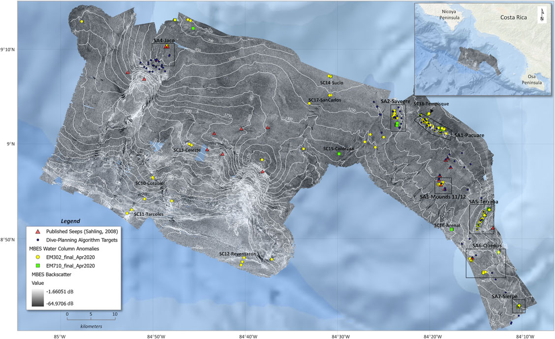
FIGURE 1. Multibeam backscatter and bathymetry contours (meters) of full study area. Map records MBES water column anomalies identified in this study, previously published seep locations (Sahling et al., 2008), and targets identified by Spock for investigation during the expedition. Map shows uneven distribution of water-column anomalies with depth as well as tendency to occur in clusters. Many anomalies found in areas of previously identified seeps, but new locations of seepage are also observed. Seep Clusters (SC) and Arrays (SA), defined to reflect hierarchy in organization of seep features, are labeled with Costa Rican river names for purposes of communication.
The expedition used the ship’s Kongsberg EM302 and EM710 MBES instruments for mapping and the SuBastian1 remotely operated vehicle (ROV) for seafloor observations and sampling. In addition, two autonomous underwater gliders (AUGs) were deployed during the cruise: AUG Nemesis was deployed for most of the cruise with a magnetometer and conductivity, temperature and depth (CTD) sensor payload to test vehicle endurance improvements, and AUG Sentinel (Duguid and Camilli, 2021) was equipped with a Doppler sonar and CTD to test and maintain an adaptive sea bottom-conforming flight path. Automated interpretation and planning processes were deployed and tested to identify potential seep targets, to arrange those targets into ROV and AUG transects that optimized scientific rewards under operational constraints, and to manage and optimize multiple, sometimes simultaneous operations in the most efficient manner possible. Lastly, an automated motion planner relying on machine vision was implemented for ROV robotic arm manipulation. Initial ROV missions used considerable information from previous studies and the geoscience staff, while later transects were planned by the automated planning processes using the ladder framework combined with preliminary real-time data collected during the expedition.
The southern coast of Costa Rica has been the focus of nearly 2 decades of seep-related research, including multiple geophysical cruises, multiple ROV and HOV expeditions, and three ODP/IODP drilling expeditions. Those studies greatly advanced understanding of deep fluid sources at subduction zone plate interfaces (e.g. Hensen et al., 2004; Mau et al., 2007; Ranero et al., 2008; Kluesner et al., 2013; Riedinger et al., 2019), and identified a number of seep sites at which deep-sourced fluids might be sampled (e.g. Füri et al., 2010). As such, rather than having to develop new insights into the way seep systems work, we were able to use the existing information from Costa Rican seeps, supplemented with information from Hydrate Ridge offshore Oregon (e.g. Torres et al., 2009; Baumberger et al., 2018), and seep processes in general to guide our geologic strategy to help support the primary technology demonstration objectives. To pursue this strategy, we revisited known and previously studied seep sites (e.g., Bohrmann et al., 2002; Linke et al., 2005; Mau et al., 2006; Klaucke et al., 2008; Sahling et al., 2008) as well as documenting newly discovered seep sites.
A Ladder of Seeps was constructed to provide a framework for relating data acquisition and interpretation to scientific objectives (Figure 2), and in our case identifying seeps with a higher likelihood of emitting deep-sourced fluids. The framework could be modified for alternative objectives, like searching for hydrothermal vents, cold seeps with microbial mats, or seep surveys to estimate fluid flux. While achieving the goal of identifying deep-sourced seeps with high confidence only from measurements above the sediment-ocean interface is unlikely because of fluid dilution effects, using the ladder can increase the likelihood of finding these seeps using low-resolution screening data, and thus improve the chances that deeper sediment cores taken at the seep sites will recover deep-sourced fluids. The ladder includes measurements common on marine geophysical vessels and conducted on the R/V Falkor expedition used to identify seafloor features common in seep environments such as carbonate crusts, mounds, seep biota, and bubbles. No single measurement is sufficient to identify a deep-sourced seep, but the ladder provides a framework to help an investigator determine which measurements to collect at each stage of analysis and understand the combination of measurements that increases the likelihood of identifying seeps with deep-sourced fluids.
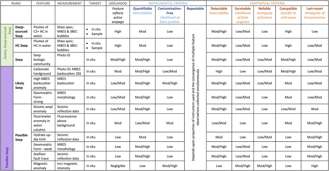
FIGURE 2. Ladder of Seeps. Conceptual framework for exploring for specific seep types. Lower part of table defines exploration progression from Possible to Likely Seep, and upper part describes different types of active seeps with each higher rung representing subset of seep type below. Table columns include type of feature observed in nature (Feature), what type of Measurement is made to detect feature, whether measurement is made above seafloor or below (Target), and Likelihood that proposed Feature describes Ladder Rung. Issues of Instrumental Criteria include whether proposed Feature is Quantifiable (Detectable), Contamination-Free (False Positive) and Repeatable. Contextual Criteria represent an explicit evaluation of scientific method by considering whether feature is Detectable, Survivable (False Negative), Reliable, Compatible (i.e. specific to natural cold seeps), and Last-Resort interpretation (i.e. does evidence refute all other possible hypotheses). Deep-sourced fluids are placed at top of ladder in this instance to identify locations for earthquake studies, but ladder could be modified for other scientific objectives.
The Ladder (Figure 2) assumes no initial knowledge of a given survey area. It presents a hierarchy of rungs that ascend from no knowledge to Possible Seep, on to Likely Seep, and then to Confirmed Seep, Hydrocarbon Seep (i.e. one with alkane gases), and Deep-Sourced Seep on the top rung. Note that, in general, the cost of data acquisition to ascend each rung increases. Each rung is achieved by the positive identification of a particular seep Feature and the corresponding measurement used to identify the feature. The target column indicates whether the measurement is made above the seafloor (in situ) or from subsurface fluid samples. The Likelihood column reflects an opinion about whether the specific measurement achieves the higher ladder rung (e.g. hydrocarbon seepage); note that aggregate measurements at a Possible Seep rung can increase Likelihood above that of any individual measurement. The Instrumental Criteria include assessments of whether the feature is quantifiable (detectable) with any particular measurement, at the physical and temporal scales of measurement (e.g., what chance does a passing ship have to observe a time-varying bubble flux?), whether the measurement is contamination-free (i.e. likelihood of false positive), and if it is repeatable. For example, magnetic anomalies are poor indicators of seeps because seep features are neither quantifiable (i.e. a seep must precipitate a magnetic mineral in sufficient volumes to rise above background noise) nor contamination-free (inversion of magnetic data allow multiple geologic scenarios). On the other hand, identification of a seep biologic consortium (e.g., microbial mats, tubeworms, clams, and mussels) is possible from photographs of the seafloor, and the chance of mis-identification (false positive) from photos is low.
The contextual criteria address how easy the sought-for feature is to recognize in the environment being analyzed and with the tool being used. Microbial mats, for example, are often detected by the color contrast between mats and surrounding sediments so detection will be better when the contrast is greater. Hydrocarbon plumes in the water column have variable survivability because of the time-varying nature of seeps and the ability of currents to disperse plumes. On the other hand, if a bubble plume is observed (reliable), confidence in the discovery of a seep is high. And bubble plumes are associated with few other marine geologic features (compatible), although some seep biota are found in other environments (e.g., mats associated with organic-rich sediments or slumps). The final column (last-resort) aggregates all of the instrumental and contextual criteria used to identify a particular feature to evaluate the ambiguity of interpretation, or whether plausible alternative explanations for the measurement are permitted.
Seafloor and acoustic backscatter mapping address the second rung of the ladder (Likely Seep; Figure 2). These data were collected with a 30 kHz Kongsberg EM302 MBES and a Kongsberg EM710 operating at 70 kHz on the R/V Falkor (Schmidt Ocean Institute cruise FK181210)2. While the survey covered 2,967 km2 of seafloor in water depths from 225 to 3,616 m, the ship-track covered some areas multiple times as the ship was repositioned for AUG deployment/recovery and ROV operations.
The resulting seafloor map was created by oversampling the EM302 data; swaths on adjacent lines overlapped by ca. 20% in order to accommodate reasonable water column illumination. The EM710 was activated in water depths <1,000 m, but a ship-track dictated by EM302 data collection caused gaps between adjacent EM710 lines with a narrower beam footprint. Seafloor picks from both datasets were combined to create a bathymetric map gridded at 30 m even though local areas with EM710 data could allow a bathymetric grid at 15 m.
A seafloor backscatter map was constructed at a resolution of 15 m using standard methods in Qimera3 (Supplementary Material). We applied a generic processing workflow in order to generate real-time backscatter maps for ROV operations planning and Spock analyses and recognize that further data processing might provide additional data insights. Maps were created in both geographic coordinates and projected onto UTM projection WGS 84 UTM Zone 16 N.
Water column data, which address the fourth rung of the ladder (HC seep; Figure 2), were collected with both EM302 and EM710 MBES instruments, and water column anomalies were systematically identified with the Feature Detection algorithms in FMMidwater4 software. More detailed descriptions of filtering parameters applied and interpretation strategies employed are given in Supplementary Material and Supplementary Table S1.
Point Clusters defining water column anomalies were imported into Fledermaus and further filtered using the Clustering Algorithm tool to eliminate any remaining noise and to separate multiple anomalies contained within a single Point Cluster. Given the resulting character, shape, amplitude distribution, and position in the water column, each resulting anomaly was labeled a high, medium, or low confidence bubble plume (Supplementary Table S8). Low confidence anomalies were excluded from further analysis.
To aid in seafloor mapping, the source location of every water column anomaly was estimated with the Fledermaus Cluster Summary Object Tool by regressing a 3D line through the points and extrapolating that line to the seafloor. When poor or no regressions resulted, the seafloor source was manually estimated. For each resulting interpreted plume, we compiled a seafloor X, Y, Z location, recorded the number of points within the interpreted plume, defined the position of the base of the plume in the water column (Low, Moderate, or High), and interpreted a Low, Moderate, or High confidence in the final seafloor source interpretation.
The Sentinel AUG was deployed on two missions using an onboard adaptive mission controller, which enabled the AUG to transition autonomously from water column profiling in waters >1000 m deep, to a bottom-following behavior, wherein the AUG maintained an altitude band of between 5 and 50 m altitude above the seafloor. This behavior enabled the AUG’s downward-looking 600 kHZ phased array Doppler velocity log (DVL) to interrogate both the water column and seafloor below the vehicle. Post-processing of acoustic ping ensembles (bin velocities and acoustic return intensities) for each of the four beams was merged with synchronized vehicle pose using a shear method process similar to that described by Visbeck (2002) to estimate water column velocities with 1 m vertical resolution. Thresholding of individual beam intensity while accounting for through-water acoustic attenuation and distance-dependent beam spreading enabled identification of seafloor contacts and water column acoustic anomalies attributable to bubble plumes (further details about method described in Supplementary Material, Sect. 2.7). Water column and seafloor (i.e., bottom lock) velocity estimates were then integrated with AUG dead-reckon navigation estimates to generate a DVL-odometry estimate of vehicle track which constrained vehicle position uncertainty to within approximately 15% of distance traveled. Using this DVL-odometry estimate, locations and intensities of seafloor and water column acoustic contacts were mapped to identify possible seep bubble plumes and carbonate hardgrounds. It is noteworthy that this AUG mapping process required only 20 J/m of linear survey, allowing for unattended mapping operations of up to weeks in duration before requiring AUG recharge or recovery.
A series of automated algorithms formulated around Bayesian statistics, information theory, and multi-vehicle routing with time windows were developed and combined to identify cold seeps using bathymetric, acoustic backscatter, and water column data collected in real-time. These algorithms are collected into an application informally called Spock. Use of Spock was intended to plan ROV dives to increase the number of seeps visited during a dive (i.e. to advance sites from Possible Seeps to confirmed Seeps on the Ladder of Seeps). The success of predictions was tested by human observations from an ROV, and data obtained early in the cruise were used to update probabilities with the intent of improving prediction success on each subsequent ROV dive.
The operational significance of our approach is that newly acquired bathymetric, backscatter, and preliminary water column data were combined into ROV seep targets in an objective and reproducible manner in as little as 2 h, faster than analyses done by hand. The algorithmic approach identified novel candidate locations that may have otherwise been overlooked and was able to extract in a quantitative manner the relative strengths of evidence for seepage while at the same time evaluating sites without seeps, thereby strengthening the certainty of places to avoid.
Spock operates by using observation data and evidence of seep presence to learn the parameters of a Bayesian discrete undirected graphical model (Buntine, 1994) that correlates seep presence with local bathymetry and backscatter. Random samples of the model parameters that were consistent with the data were generated using the Metropolis Hastings algorithm (MacKay, 1998), which were then used to compute probabilities of seepage presence. Scores were assigned to visiting each site, which were computed according to Bayesian multi-armed bandit algorithms (Kaufmann et al., 2012; Lattimore and Szepesvári, 2020). The Bandit algorithms assigned a better score if a site had a high probability of seepage and if it displayed data signals that were uncommon in the data set. For example, pockmarks are uncommon in the Costa Rica data set so the influence of pockmarks on seepage probability was uncertain. Higher scores directed dives towards pockmarks so that posterior probabilities were better refined. Bandit algorithms describe how to select the relative weights of seep probability and uncertainty, and prove that these strategies result in more seeps found than only visiting the sites with the highest probability. A final stage solved for a connected track that maximized the cumulative score of all visited sites, limited by how far the ROV could travel over the time allotted to the dive (Desrosiers et al., 1995).
The initial Bayesian framework applied to the first dive was based on expert opinion trained on published data for cold seeps on the Costa Rica margin (Sahling et al., 2008). The Sahling et al. (2008) study identified 112 candidate seep sites associated with mounds, pockmarks, and faults visible in the bathymetry map, as well as high backscatter. The sites labeled with active seepage in the Sahling et al. (2008) data set were marked as seeps for algorithm training. For the planned dives, sites with higher probability of seepage were identified based on the generated bathymetric and acoustic backscatter maps. Because prior studies indicated that seeps were frequently associated with mounds, pockmarks, faults visible in the bathymetry map, and high backscatter, locations with evidence of these bathymetric features and/or backscatter above background levels were identified from the map and used to build a candidate set of dive sites.
Bubble plumes identified from MBES water column data provided additional evidence for seepage, but few plumes were identified at the time of dive planning. Across all algorithmically planned dives, 19 plumes were available. When plumes were available, the location of the seafloor source was visually estimated from the base of the plume. The estimated source locations were added to the candidate site set if they did not align with candidates derived from bathymetry and acoustic backscatter.
Initial ROV dives were planned by hand, focused on seep areas defined by others, and took valuable time from other activities early in the expedition. Five subsequent ROV dives and two Sentinel AUG missions were planned with Spock’s assistance. Every potential dive site was labeled in terms of features that were present, absent, or unmeasured, including mounds, pockmarks, high backscatter, and bubble plumes. The presence of high slope was hypothesized to be correlated with seepage and was also included because the Bayesian approach allows consideration of primitive hypotheses. Every possible combination of features was modeled as having a fixed probability of a seep being present. Over the course of the cruise, Spock learned the seep presence probabilities, and then used that information to identify the sites with the highest probability of seepage. Each dive selected 2–10 sites within close proximity to visit out of between 10 and 40 candidate sites that could be reached on a given dive. The Spock predictions were checked by hand to validate that dive targets were logical and of scientific interest.
Formulation of site selection as a multi-armed bandit problem balanced visiting sites that best improved seep presence probabilities against visiting sites with a high estimated probability of seepage. Multi-armed bandit algorithms produce strategies for sampling that maximize the expected reward drawn from unobserved probability distributions; in other words, when initial probabilities are based on global knowledge, how can that knowledge be refined in a given location to maximize success in finding seeps? In this case, the reward was 1 for a seep being present, and 0 otherwise, and the multi-armed bandit algorithm selected the combinations of features to visit to maximize expected reward. Among the many available multi-armed bandit algorithms, we used Information Directed Sampling (IDS; Russo and Van Roy, 2018). IDS provides a score for each possible site and directs that the site with the lowest score should be visited. By employing this approach, we sought to maximize opportunities for advancing on the Ladder of Seeps. IDS was chosen from a selection of bandit strategies because it is suitable for Bayesian problems, which allowed us to use priors drawn from previous observations in the area and model suspected correlations. Furthermore, IDS yields an explicit quantification of the relative contributions of seep likelihood and probability refinement towards score, making Spock’s recommendations more interpretable. While IDS coupled with our conditional independence model gave scores for each dive, the choice of which sites to visit was still a combinatorial problem. Any number of sites could be visited if a path between them could be produced that was consistent with the average underwater speed of the vehicle and the time allotted for the dive. The optimal dive that minimized the IDS score was solved as a discrete search problem. Bounds on the score of any path that included a set of sites were computed, which allowed the optimal path to be found without explicitly evaluating all possible paths.
The term “seep” is applied to phenomena at a range of scales from the area of an instrument placed on the seafloor to measure fluid flux (e.g., Tryon et al., 1999) to a km-scale map feature (e.g., Klaucke et al., 2008; Sahling et al., 2008). In order to test predictions of seep locations with Spock, a seep must be defined at a scale (50 m) that can be evaluated. To account for different spatial scales, a mapping hierarchy was defined and applied to data derived from bathymetry, acoustic backscatter, and interpreted seafloor sources of plumes. The smallest entity in the hierarchy is a Seep that is limited to a seafloor dimension of <5 m based on the size of seeps on land. Fluid flux from an individual seep is variable over multiple timescales (e.g., Tryon et al., 1999, Tryon et al., 2002). The scale of a seep is much smaller than mapping resolution.
Seeps occur in clusters on the seafloor rather than being randomly distributed, so individual seeps that occur near one another were collected into Seep Clusters. The scale of Seep Clusters is conditionally defined to lie between >5 m and <10 s to 100 s of meters based on observations of cold seeps on land (Gouveia and Friedmann, 2006; Barth and Chafetz, 2015) and includes multiple backscatter pixels. The boundary of a seep cluster occurs at a transition from a higher to lower seafloor backscatter value. To verify the significance of this boundary, the mean backscatter value is computed for each interpreted seep cluster and compared with the mean backscatter value of the surrounding region. Rather than use raw backscatter values, those values were binned and re-gridded at 50 m resolution in order to reduce the influence of data artifacts.
Seep Clusters similarly exist in groupings, designated as Seep Arrays. Seep Arrays sometimes occur around a clear bathymetric feature like the Jaco Scar (Seep Array 4; Figure 1), or sometimes in linear arrays that might reflect seepage along high-angle faults (Seep Array 2; Figure 1). The purpose of defining Seep Arrays is to help raise questions about sub-surface structure that might promote fluid flow. Costa Rican river and lake names were assigned to Seep Arrays to assist in communication. Given the desired relationship between Seep Arrays and geologic structures, dimensions of Seep Arrays are defined between 100 s of meters and 1–5 km.
At sites visited by the ROV, geologic and biologic observations were compiled using Squidle+5 open-source software that allows real-time capture and annotation of ROV observations, coupled to flexible data storage for post-cruise analysis (e.g., Proctor et al., 2018). Squidle+ was expanded to include geologic observations like the state of the seafloor and structures observed (e.g., rubble). By using Squidle+, the geoscience participants generated consistent observations from site to site and between observers. The observations were captured within a classification scheme established and used by NOAA on the Okeanos Explorer (e.g., Gomes-Pereira et al., 2016), modified to include additional observations that help establish the position of each site on the Ladder of Seeps. Figure 3 shows examples of the main seafloor features logged in Squidle+ during ROV dives. Biologic observations remain generic because of the geoscience expertise onboard, but the Squidle+ database allows more detailed interpretations. The classified ROV observations were captured in a geospatial mapping and analysis system and integrated with seafloor bathymetry and backscatter maps, MBES water column analyses, and sample data to build the spatially related Seep Clusters and Seep Cluster Arrays described above.
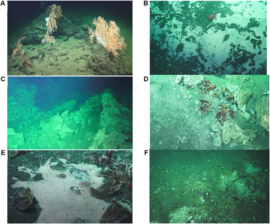
FIGURE 3. Seep observations photographed by ROV. (A) Corals affixed to carbonate crust outcrops, Dive SO204 (SA4: Jaco); (B) Methane bubble stream rising out of edge of microbial mat, Dive SO206 (SA1: Pacuare); (C) Jagged carbonate crust outcrops, Dive SO204 (SA4: Jaco); (D) Clam colony nestled along edge of carbonate crust and adjacent thin microbial mat covered by snails, Dive SO204 (SA4: Jaco); (E) Thick microbial mat fringed by clams, Dive SO210 (SA2: Savegre); (F) Tubeworms growing from carbonate crust outcrop and flanked by clams, Dive SO208 (SA3: Mounds 11/12). Specific photo locations identified in Supplementary Materials (Seep_Array_Documentation.pdf).
Seafloor conditions were recorded by the CTD onboard the ROV. The ROV was also equipped with a double focusing membrane inlet mass spectrometer operating as payload to identify water column chemical anomalies in a functionally similar configuration to that described in Feseker et al. (2014), Camilli et al. (2010), and Camilli et al. (2009). A 6 mm diameter polyurethane sample introduction tube connected to the length of the manipulator arm and backed by a small impeller pump provided continuous sample introduction to the mass spectrometer’s inlet. Analytes of interest included methane, ethane, hydrogen sulfide, propane, carbon dioxide, and benzene, which were observed in real-time as molecular ion peak and ratio signatures at m/z: 15, 27, 34:32, 43, 44, and 78, respectively. Ion peak height data were post-processed with a 10- min temporal “box” filter centered at ± 5 min to identify the onset and approximate magnitude of anomalously increased ion peak intensities above background levels.
Pore water and headspace gas samples were obtained from ROV push-cores using standard methods (Supplementary Material). Preserved pore water samples were analyzed for major and minor elements and oxygen and hydrogen isotope ratios at the University of Bremen. Methane concentrations were measured from headspace gas samples and from CTD water samples at the University of California, Santa Barbara by gas chromatography, and stable carbon isotope ratios of methane were measured at Woods Hole Oceanographic Institution. Because analytical precision is much greater than the precision required for the interpretations reached in this study, details of the methods used are documented in Supplementary Material.
Water column anomalies that satisfy criteria of size, shape, amplitude distribution, and position in the water column are interpreted as bubble plumes (Anderson, 1950; Sullivan-Silva, 1989; Medwin and Clay, 1998) and offer the most substantive evidence for seafloor seeps from a sea-surface measurement. We recorded 209 unique bubble plumes that are tabulated in Supplementary Table S2. Information in those tables include the interpreted seafloor source of the bubble plume (X, Y, Z), the date and time it was observed, the number of points attributed to the bubble plume, our confidence that the water column anomaly is a bubble plume, and the MBES source of the observation. Some plumes were recorded by both MBES systems, and some plumes were recorded more than once.
The seeps are unevenly distributed in depth over the study area (Figure 4). Comparing plume occurrence with the distribution of bathymetry depth nodes suggests that there is no significant coverage bias in these results (i.e. ca. 5 × difference in number of depth nodes in survey area inside the upper and lower depth limits). In addition, small-moderate plumes are present at all depths, but the largest plumes are found where plumes are clustered in depth. A gap in plume occurrence is found between ca. 800–1000 m.
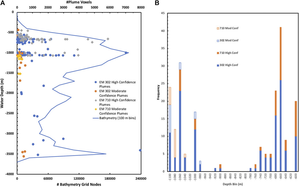
FIGURE 4. Observed depth distribution of water column anomalies (bubble plumes) for EM302 and EM710 datasets. Note that EM710 sonar deactivated in water depths > ca. 1000 m. (A) Bubble plumes plotted as number of voxels (points) in final Fledermaus model vs. depth for High and Moderate Confidence plume interpretations. Bottom axis (blue curve) records number of bathymetry nodes in 100 m bins to test for possible coverage bias (e.g., between 800 and 1000 m where few plumes identified). (B) Histogram of EM302 and EM710 High and Moderate Confidence bubble plumes binned in 20 m increments. Note paucity of observations between 800 and 1000 m water depth.
Water column anomalies identified in AUG sonar data correspond in space to anomalies identified with ship-based MBES data (Figure 5). While the data were collected at a much higher acoustic frequency with vastly different spatial coverage and resolution, processed in a different way, and collected on different days than the ship recordings, the correspondence in seep source location between AUG and MBES data is remarkable.
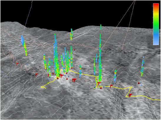
FIGURE 5. AUG sonar observations of bubble plumes in SA1: Pacuare (red flags) compared with EM302 plume observations (pyramids represent seafloor source and blue-green-yellow-red colored stalks are bubble plumes with red colors indicating amplitudes of 3–10 dB and light blue amplitudes between −30 and −45 dB). Pink lines represent AUG flight path. Note that plumes identified at bottom of any flight cycle. Yellow line is ROV Dive 205/206 path. Closely spaced bathymetric contours in dive area at 10 m increments; shallowest depth contour at top of dive site is −660 m, and shallowest depth contour at top of image is −600 m. VE = 3x. View to NE. Note that given AUG navigation uncertainties, reasonable correspondence found between EM302 and AUG plume interpretations.
Application of the mapping hierarchy led to the identification of seven Seep Arrays from the combination of ship-based bathymetry, backscatter intensity, and water column anomalies (Figure 1). Four of the seven arrays occur in association with seafloor mounds, faults, and landslides identified by previous studies (Jaco, Quepos, Sierpe, and Mounds 11/12). A fifth array (SA2: Savegre) sits just outboard from a long, curved, steep slope that may coincide with a structural boundary. The remaining two arrays (Pacuare and Terraba), as well as several individual water column anomalies in the NW corner of the study area, occur at ∼600–650 m water depth, near the intersection of the base gas hydrate stability zone with the seafloor.
Two to eight Seep Clusters have been mapped within each array. Cluster maps, high-resolution seafloor maps, raw and reclassified backscatter maps, and any additional data used to map the clusters are found in Supplementary Material (Seep_Array_Documentation.pdf). The clusters range in area from 0.01 to ∼1 km2, although most are <0.1 km2. Most clusters include all key mapping features: water column anomalies, relatively high backscatter intensities, and some seafloor bathymetric expression of a fluid pathway, e.g. mound, fault, break-in-slope, pockmark. A few clusters have no water column anomalies and were mapped from ROV observations (described below). Because Seep Clusters are smaller than Seep Arrays, the bathymetric morphology can change with the scale of the observation. For example, the clusters mapped in SA3: Mounds 11/12 consist of a SW plunging ridge, a gentle slope, and domes (mounds), while individual seeps are found on slopes, ridges, or mounds. Figure 6 illustrates the mapping of two clusters that exemplify differences in attributes that may influence predictions made by Spock. SA1: Pacuare (Figure 6A) comprises six seep clusters ranging from 0.01 to 0.4 km2, each with a minimum of 2–3 water column anomalies. At the scale of the array, each cluster occurs along a bathymetric ridge, although local topography around individual seeps may be flat. The mean backscatter class value for each cluster is above local background, although within standard deviation, particularly for the smaller clusters. In contrast, SA7: Sierpe (Figure 6B), in the southeast of the study area, contains just two seep clusters, ranging from 0.01 to 0.03 km2. Both have water column anomalies, but backscatter intensity is similar to background. The high-resolution characteristics of these arrays are described in the next section (ROV Mapping).
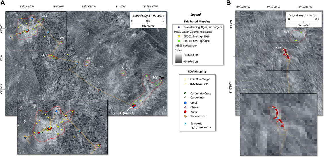
FIGURE 6. ROV mapping of representative seep clusters. Maps illustrate MBES backscatter and bathymetric contours (meters) for two sites with different seep characteristics. Seep clusters defined from ship-based mapping are defined by red polygon outlines, labeled by Seep Cluster number. ROV observations annotated in Squidle + are superimposed. (A) Seep Array 1—Pacuare contains six clusters between 600 and 650 m water depth. Four clusters (SC1-3, SC6) were occupied during ROV dives SO205/SO206, and display heterogeneous distribution of carbonate crusts, corals, bacterial mats, and tubeworms that occur in regions of higher backscatter. SC1 characterized by mound-shaped geometry (inset map) while remaining clusters occur on topographic ridges, flats, and valleys. (B) Seep Array 7—Sierpe contains only two seep clusters between 690 and 720 m water depth, dominated by bacterial mats, with no carbonate crusts. Seafloor topography flat with backscatter values close to background (inset map).
In addition to Seep Clusters mapped within each of the arrays, we also identified individual clusters independent of the arrays. These clusters were defined in regions where two to three water column anomalies were identified within a few hundred meters to a kilometer of each other. The proximity of the seeps in these clusters suggests a broader geologic control, but that control was difficult to identify from the available data, hence they were given no formal Array designation (e.g. Seep Clusters Reventazon, and Tarcoles, adjacent to the trench; Figure 1).
ROV mapping of individual dive sites provided the critical piece of information that allowed a target site to move from Likely Seep to Seep on the Ladder, based on observations of seep biologic communities and carbonate hardgrounds (Figure 2). The ROV dive sites visited during this expedition display the authigenic carbonates and associated biologic communities typical of seafloor seep environments and observed by previous expeditions to this region (e.g. Bohrmann et al., 2002; Mau et al., 2006; Klaucke et al., 2008; Sahling et al., 2008; Levin et al., 2015). Generic descriptions of the seep communities were sufficient to achieve the Ladder of Seeps objectives for this study, but the full expedition database is archived with the R2R repository6 and can be revisited if a more detailed description of seep characteristics is warranted for future study. Table 1 records observations of biologic communities and authigenic carbonates discovered at each ROV site. Complete tables of Squidle + annotations can be found in Supplementary Material (Annotations-ROV Excel files). The seep-related biologic communities observed in the study area included clusters of siboglinid tubeworms, abundant aggregations of vesicomyid clams, rare mussel beds, deepwater corals, and bacterial mats. Most are spatially associated with carbonate crusts, boulders, and mounds (Figure 3). Seep succession models (e.g. Cordes et al., 2008; Lessard-Pilon et al., 2010; Bowden et al., 2013; Guillon et al., 2017) suggest that bacterial mats are the earliest to develop at new seep sites. Subsequent precipitation of authigenic carbonate permits mussel colonization, and declining sulfide seepage allows tubeworm colonies to begin to dominate. Vesicomyid clams are prominent members of seep communities but tolerate a large range of chemical fluxes and concentrations, and as such, are less diagnostic for seep succession processes. They are, however, thought to enhance the anaerobic oxidation of methane, which can in turn accelerate the formation of the authigenic carbonates needed as substrates by other fauna (Guillon et al., 2017). Deepwater corals often grow on authigenic carbonates derived from hydrocarbon seepage, but their nutrition is considered to come from non-seep sources (Cordes et al., 2008) and may be concentrated in areas where seeps are no longer active.

TABLE 1. Summary of ROV seep observations.
Approximately 30 Seep Sites were documented during nine ROV dives (Table 1). Detailed maps of each dive site are included in Supplementary Materials (Seep_Array_Documentation.pdf). Figure 6 illustrates the key observations at two new sites with characteristics typical of those used to promote placement of a seep on the Ladder. SA1: Pacuare (ROV dives SO205/SO206; Figure 6A) comprises six individual seep clusters ranging from 0.01 to 0.4 square kilometers, each with a minimum of 2–3 water column anomalies. The seeps all occur at 652–695 m water depth (Supplementary Table S2), within 100 m of the intersection of the base gas-hydrate stability zone with the seafloor (Bohrmann et al., 2002, and Mapping Seafloor Conditions). At the scale of the array, the seeps occur along a series of dip-parallel topographic ridges, although local topography around individual seeps may be flat. The more well-developed clusters have mound-shaped topography and high backscatter intensity consistent with well-developed authigenic carbonates. Because additional seeps and seep clusters were identified by post-cruise comprehensive water column analyses, two seep clusters (SC4-5) lie beyond the ROV path. At the remaining four seep clusters (SC1-3; SC6), characteristic authigenic carbonates and seep biologic communities were observed (Figure 6A). SC1 is one of the largest seep clusters in the study area and consists of 19 individual seeps with an overall cluster diameter of ∼1 km. The biologic communities suggest that the most active area of seepage is near the center; the edges of the cluster are dominated by authigenic carbonates and corals, whereas the central area contains abundant bacterial mats, tubeworms, and authigenic carbonate crusts. Occasional observations of minor carbonates and/or mats along the dive pathway suggest the emergence of new seeps, but the features were likely too small to be identified as targets by Spock. SC2 and CS3 also display only rare carbonates and minor bacterial mats but do have water column anomalies. SC6 is another composite of individual seeps with 14 water column anomalies. The ROV path intersected only the southern portion of the cluster, where we found a heterogeneous mixture of carbonate crusts, bacterial mats, and minor corals, suggesting a complex distribution of seep activity.
In contrast to SA1: Pacuare, SA7: Sierpe (Dive SO209; Figure 6B) contains only two seep clusters at ∼700 m water depth, ranging in area from 0.01 to 0.03 km2. Water column anomalies were recognized during the initial shipboard processing of MBES data in this area. Those anomalies, coupled with published subsurface indicators of fluid flow (Kluesner et al., 2013), resulted in a strong pre-dive prediction of seep targets by Spock. Without those observations, the pre-dive prediction would have been much weaker, as neither the seafloor topography nor the backscatter intensity provided any strong indicators of seepage. The ROV dive identified abundant bacterial mats, and fields of vesicomyid clams, consistent with a robust seep in the relatively early stages of development. No carbonate crusts were observed.
A synthesis of ROV mapping at the dive sites confirms the presence of biologic communities that would designate a seep as Active (Figure 2) at approximately two-thirds of the sites (Table 1). At six of those sites, however, the communities were dominated by deepwater corals, suggesting that at those specific sites, seeps may be dormant.
Seafloor conditions were recorded by the CTD onboard the ROV, and the temperature and depth readings are used to document seafloor conditions (Supplementary Table S3; Supplementary Figure S1). While temperatures vary at water depths greater than 1000 m, there is good convergence in observations at 700 m. Combining these observations with a calculation of the hydrate stability field (Dickens and Quinby-Hunt, 1994) leads to an inference of the top of the hydrate layer at 580–600 mss, identical to the depth range reported by Bohrmann et al. (2002).
The purpose of the porewater and gas analyses is to identify samples with possible deep fluid components, the top rung in the Ladder of Seeps, and to gather additional information about the longevity and frequency of individual seeps. Sample locations are recorded in Supplementary Table S4. We applied a process and fluid source framework developed in previous work (e.g., Whiticar, 1999; Chan and Kastner, 2000; Kopf et al., 2000; Silver et al., 2000; Grant and Whiticar, 2002; Lückge et al., 2002; Milucka et al., 2012) that include water modified by diagenesis and very low-grade metamorphic reactions (ultimate goal), water from deep compaction processes (>1 km), and hydrocarbon gas generated by thermal cracking of organic matter. Shallow fluid sources and processes that alter both shallow and deep fluids include water produced from shallow (<1 km) compaction, biogenic gas generated by microbial processes, bacterial methane oxidation, and hydrate formation and disassociation. Given these limited goals and the limited time and geoscience staff resources available on the ship, we only collected samples that were analyzed onshore and excluded ship-based analyses that might better define microbial processes (e.g., bicarbonate concentration). We also only took 1–2 samples in each core rather than the more conventional profiles because we collected short cores (ca. 25 cm) and had insufficient time for more sampling.
Most cores consist of only a single porewater analysis (Table 2), although samples SO210-01, -03, and -06 all include an upper and lower sample. In most cases, porewaters were extracted from a depth of 10–15 cm in the core. Ion concentrations are presented with respect to their concentration in seawater.
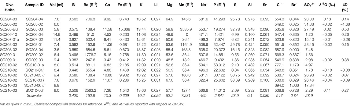
TABLE 2. Inorganic pore water chemistry results.
The following cations are enriched in sampled pore waters with respect to seawater: B, Ba, Fe, K, Mn, Na, P, and Si (Table 2). Only one sample (SO209-03) has less B than seawater, and two samples (SO206-04 and SO-210-03) have less Ba than seawater (two samples have the same concentration of Ba as seawater). All samples have more Fe than seawater (up to 250 × enrichment), and all samples are enriched in Mn (up to 500 × enrichment) except for one sample (SO206-04); which has none. Extreme Fe and Mn enrichments occur in the same sample (SO-205-03). All samples are enriched in P with an enrichment up to 15 × (SO204-04), except for SO206-04, which has half seawater concentration. K and Na are modestly enriched in all samples (up to 1.4 × for K and 1.3 × for Na), but sample SO209-03 has a slight Na depletion. Si is enriched in all samples up to a factor of ca. 5 × (SO210-01).
Ca is enriched in four samples with respect to seawater, like Na and K, but in most samples, Ca is depleted with as little as 1/3 the calcium of seawater (SO209-03). Li concentrations hover around seawater values (0.020–0.031 mM), and the same if found for Mg (48.9–67.0 mM) except that the number of depleted samples is smaller and enriched samples greater, and Mg enrichment > depletion. The average Sr concentration is less than seawater, but five samples out of 14 have more Sr than seawater.
There is more S in four samples than seawater, but in other samples S is depleted to such small concentrations (0.337 mM in SO210-01) that the average of S in all samples analyzed is half of seawater concentration. Those four samples also have similar
Analyzed samples also have both more and less Cl− and Br− than seawater. In general, depletion and enrichment of both species occur in the same samples. The lowest Cl− (523.6 mM) and Br− (0.820 mM) concentrations occur in the same sample (SO207-02), and the highest Cl− (587.9 mM) and Br− (0.900 mM) concentrations also occur in a single sample (SO208-04). Note that two samples (SO210-01u and SO210-06u) have much higher Cl− (777.1 and 694.0 mM) and Br− (1.179 and 1.066 mM) concentrations. Both have Cl/Br comparable to seawater (659 and 651, respectively; SW = 651). Sample SO210-06u was too small for cation analysis, and major cation (Na, Ca, and Mg) ratios with Cl are less than seawater, while all other samples have Na/Cl > seawater and Mg/Cl < seawater and much less than other samples. We consider these values suspicious because the anion concentrations are so far from seawater values and the adjacent, lower samples have values more in line with the rest of the sample set. These two samples are excluded from further analysis, but because there is no compelling evidence for how the samples may have been altered, the values are nevertheless reported.
Oxygen and hydrogen isotope ratios of pore waters cluster around seawater values (Table 2). Oxygen isotope ratios are all within 0.2‰ of seawater, and hydrogen isotope ratios are within 2‰ of seawater. The greatest deviations from seawater are uncorrelated between oxygen and hydrogen isotope ratios.
Methane gas concentrations range from negligible to absent up to 38.5 mM (Table 3). A cluster of samples with methane concentrations <1 mM (Figure 7) consist of samples taken as background samples and seep samples. A second cluster of samples range from 1 to 10 mM, and the biggest group of samples have methane concentrations between 10 and 40 mM. Local background values range from 0.5 to 2.0 nmol/L (Mau et al., 2006). Ethane is detected in most samples, especially those from Dives 206, 207, 208, 209, and 210, but propane is detected in only three samples. Benzene occurs in all but one sample.
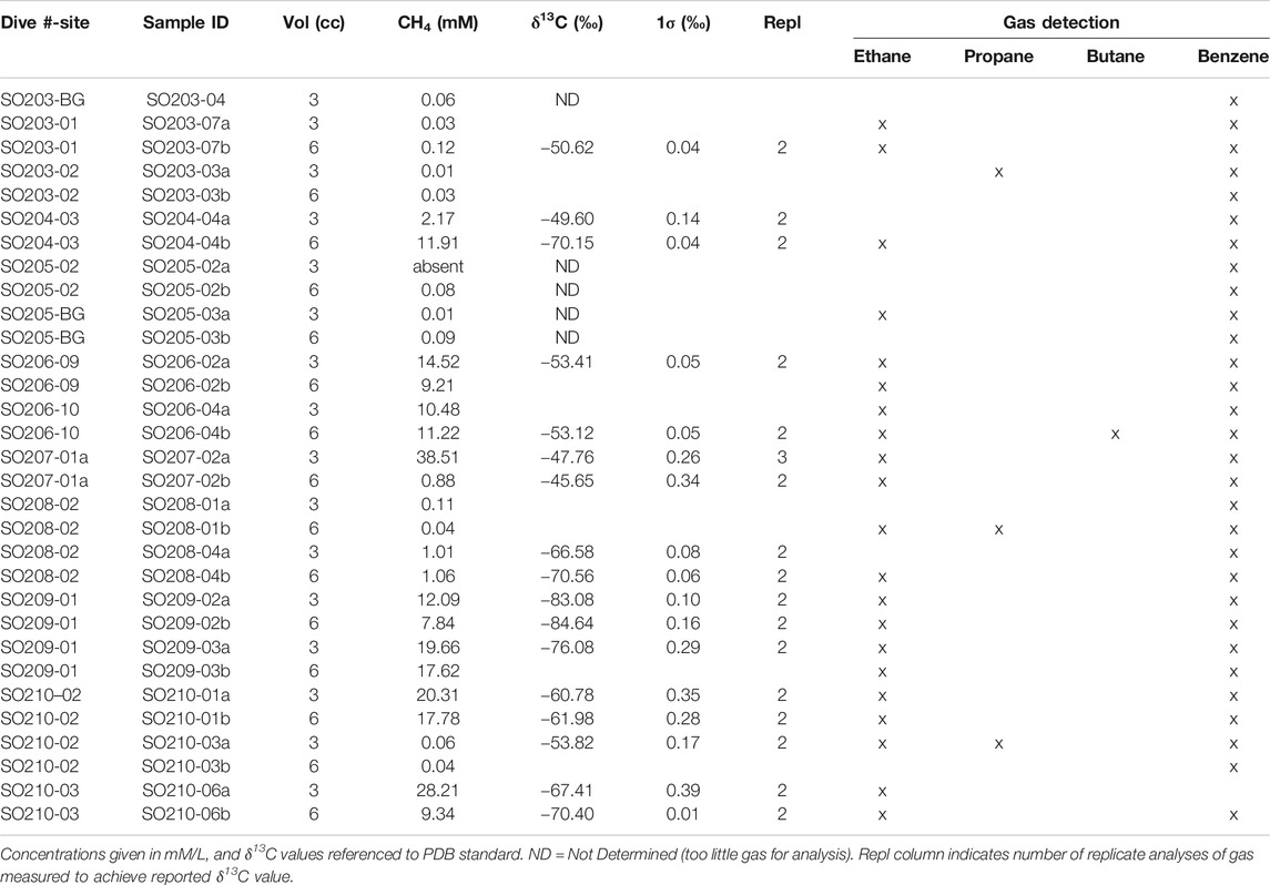
TABLE 3. Sediment headspace gas results.
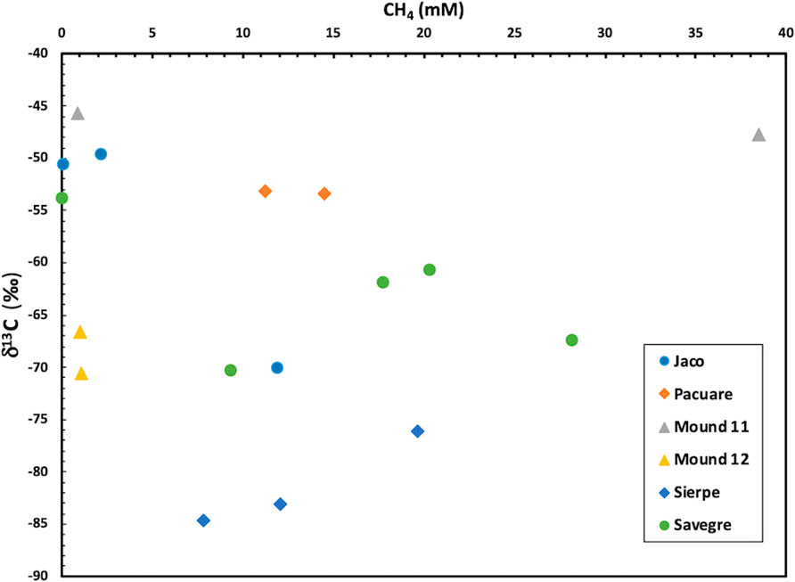
FIGURE 7. Headspace methane gas concentration vs. carbon isotope ratio of methane. Methane gas concentration ranges from negligible to 38.5 mM, and carbon isotope ratios range from −45.7 to −84.6‰ PDB, covering spectrum from thermogenic to biogenic methane. Note that two samples from Mound 11 differ in methane concentration but yield similar carbon isotope ratios; these are two samples taken at different depths in same core and suggest recent influx of methane in order to create a large concentration gradient.
Carbon isotope ratios of methane gas range in value from −45.7 to −84.6‰ (PDB; Table 3). Samples with the lowest methane concentrations (<5 mM) record isotopic ratios that range from −45.7 to −70.6‰ while samples with higher methane concentrations include the full spectrum of carbon isotope ratios (Figure 5). Two seep arrays show decreasing carbon isotope ratios with increasing methane concentration (Jaco and Savegre). Methane analyzed from Mound 11 has similar isotopic ratios but different gas concentrations, Pacuare also has similar isotopic ratios but for similar methane concentrations, Mound 12 records low methane concentrations and similar isotopic ratios, and Sierpe records an increase in carbon isotope ratio with increasing methane concentration (Figure 7).
Two CTD water samples were collected in the middle of a gas plume sampled in april and May, 2002 and interpreted by Mau et al. (2006) to be sourced from a seep on the Jaco Scar (their CTD 7). We collected samples at 1780 and 1800 mss where Mau et al. (2007) encountered methane concentrations between 50 and >200 nmol/L with an average of 85.2 nmol/L.
We found methane concentrations with an average of 52.0 nmol/L with individual values as great as 72.6 nmol/L (Supplementary Table S5). While these values are on the low end of methane concentrations measured by Mau et al. (2007), they are still well above the concentrations measured by Mau et al. (2014) outside the plume (7.1 nmol/L) and at offset background sites (1.9, 1.3, and 0.8 nmol/L). In addition, we measured C3 concentrations (average = 17.0 nmol/L) that are also above the methane background concentrations.
Water column chemical anomalies identified by the ROV’s payload mass spectrometer (Supplementary Table S6) are a rare fraction of the in-situ measurement record (n = 3170) for methane, ethane, hydrogen sulfide, propane, carbon dioxide, and benzene (representing 1.5%, 0.88%, 0.28%, 1.1%, 1.8%, and 0.32%, of the sample record, respectively). Methane, carbon dioxide, and propane anomalies exhibit correlation across all ROV dives, but the relative magnitude of these water column anomalies appear to be independent of sediment headspace gas sample concentrations collected at neighboring locations. The relative magnitudes of propane anomalies are highest when the carbon isotope ratio of methane in an adjacent sample is less negative. Of the 46 methane anomalies recorded on Dives 204–210, 36 occurred within the limits of seep clusters previously mapped. CO2 anomalies are the most abundant of the monitored analytes and had the highest discovery rate outside of seep clusters (8 of 58 anomalies). Ethane and propane anomalies are less common but were also detected on all dives, both species of anomalies occurring most often during Dives 204 and 210. All but 4 out of 28 (ethane) and 34 (propane) anomalies occur within mapped seep cluster boundaries, and the 4 exceptions are co-located with one another.
In contrast to the headspace gas samples, benzene was only detected during Dive 204 (9 anomalies) and 208 (1 anomaly). Seven occurrences of H2S anomalies were recorded on Dive 204, and one each during Dive 208 and 210. All H2S anomalies occur within seep clusters and are associated with seeps (including bubble plumes) on Dives 208 and 211.
An ROV data logging failure prevented simultaneous recording of analyte water stream temperature, precluding estimation of chemical species concentrations in absolute terms. If these anomalies are considered within the context of depth-dependent temperature records logged by same-day CTD casts, the ion peak data indicate mole fraction anomaly ranges above background of between: 10 ppb and 10 ppm for methane, 10 and 100 ppb for ethane and propane, and 1 and 10 ppb for benzene. Fragmentary temperature logs suggest that analyte fluids with elevated temperatures may have contributed to an amplification of ion intensity anomalies detected in the vicinity of the Jaco scar.
Based on ship-based mapping, ROV observations, and sample analyses, we classified each seep location as (Table 1): 1) Active Strong, requiring the presence of microbial mats or clams, a headspace methane concentration >10 mM, and optional observation of bubble plume(s); 2) Active Weak with a seep biologic community but headspace methane concentration from 1 to 10 mM; 3) Dormant, where carbonate crusts and seep biota reflect past active seepage, but for which there is no evidence of methane in headspace gas samples and microbial mats and clams that require high methane flux are absent; and 4) Non-seep, where no biologic, chemical, or physical evidence of seepage is present. This classification is necessary for algorithmic seep predictions.
Spock was used to plan most ROV dives and two AUG missions incorporating new data collected during the expedition. Early Spock dive plans were compared with independent plans constructed by humans, and subsequent plans were only checked by humans, thereby freeing staff to devote more time to new data analysis and interpretation. Further details on Spock implementation are described in Supplementary Material.
Prior to the cruise, Spock was trained on bathymetric feature presence and backscatter data derived from previous cruises on the Costa Rican active margin (Sahling et al., 2008). Features that were absent from this training data were instantiated with priors that reflected their expected influence on seep probabilities (i.e. expert opinion).
Previously detected seepage at a site and high confidence evidence of bubbles were instantiated with strong positive priors so that sites with those features were more likely to show evidence of seepage (Table 4). Medium confidence bubble signatures were instantiated with a weaker positive prior. Low confidence bubbles and high slope were predicted to influence probability of seepage, but the impact, whether positive or negative, was unknown a priori. These features were instantiated with an uninformative prior that initially did not influence predictions. The effects of those features were learned through data gathered on the cruise.
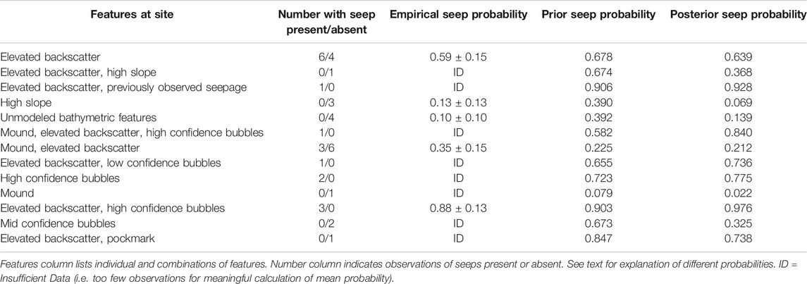
TABLE 4. Seep presence and probabilities—Spock results.
Table 4 records predicted seep probabilities for the feature combinations visited by Spock alongside truth values for how many of those sites had seepage present. Prior probabilities are based on training data only, while posterior probabilities are based on both training data and data gathered during the cruise (Table 1; Active Strong and Active Weak seeps are counted as seeps present in this analysis, and Dormant or Non-seep results are seeps absent). Empirical probabilities with 1 standard deviation (1σ = 68%) confidence intervals are computed using the Wilson score interval for binomial events (Wilson, 1927; Wallis, 2013), but most feature combinations lacked sufficient information to compute meaningful average values.
Few sites were visited for each combination of features, and this introduces significant uncertainty into empirical measures of seep presence probability. The prior probabilities of elevated backscatter, mounds with elevated backscatter, and elevated backscatter with high confidence bubbles are within the 1σ confidence interval of the empirical seep probabilities. The predictions reflect the algorithm’s belief that areas of high slope interpreted as normal fault scarps have a low probability of seepage, but high confidence bubbles are strongly associated with seeps, both of which held true throughout the cruise. Unmodeled bathymetric features, like flat seafloor, valleys, and ridges (Table 1), yielded no examples of seeps without further supporting indications (high backscatter or high confidence bubbles).
When observations from the cruise are included, modeled probabilities for seeps along high slopes and unmodeled bathymetric features drop and align better with empirical probabilities, illustrating the benefit of expanded datasets. All predictions are within the empirical 1σ confidence interval, and the mean deviation from the maximum likelihood empirical estimate drops to 0.115. The greatest change in pre- and post-cruise probabilities, both increase and decrease, arise from feature combinations that were rare or absent from the training set (e.g., high slope presence and mid-confidence bubble signatures).
In addition to generating probabilities of seepage, Spock can extract a relative measure of the impact of each feature on the probability of seepage (Table 5). The algorithm produces an expected probability of seepage conditioned on the feature being present, and a probability conditioned on seepage being absent. If the former is larger, it indicates that seepage is more likely when the feature is present, so the feature has a positive impact. In the opposite case, seepage is more likely without that feature. If the two are identical, seepage is just as likely regardless of whether the feature is present, and so the feature has no impact. While the relative influence of most features remains unchanged, the ranking of individual features shifted with the cruise results.
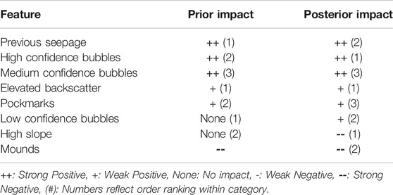
TABLE 5. Relative impacts of individual features at beginning and end of cruise.
We applied a series of new and established technologies to search for seeps on the Costa Rica accretionary margin:
1) Water column imaging from MBES and a novel AUG Doppler sonar survey
2) In situ mass spectrometry to identify hydrocarbons dissolved in ocean water that complement traditional core and CTD water analyses and help ascend a Ladder rung in our search for deep-sourced fluids
3) A decision-support system based on a Ladder of Seeps that helps define the data required to reach a specific scientific conclusion and Spock, a computer algorithm designed to use low resolution screening data and expert opinion to identify higher probability seep targets
Did these steps prove useful in improving operational efficiency and success rate in the search for higher probability, deep-sourced seep sites?
To evaluate the impact of our approach, the state of knowledge before the Falkor expedition must be defined. Sahling et al. (2008) conducted “a systematic search for methane-rich seeps at the seafloor” and documented >100 seeps. This compilation was based on 4 separate research cruises between 1999 and 2003, each cruise requiring approximately one month of ship time, plus additional bathymetric data collected earlier (Ranero et al., 2003). However, the resolution of the regional bathymetric map used for this analysis was only 100 m (von Huene et al., 2000; Ranero et al., 2008), which limited the scale of features that could be identified (>100 m). While this scale of observation was sufficient to detect the major seep clusters mapped in this study, some of the smaller seep clusters would have gone unrecognized (e.g., SC5 in SA1: Pacuare, Supplementary Materials: Seep_Array_Documentation.pdf). The Sahling et al. (2008) compilation contains a mixture of sites where seep biota confirm the need for fluid flux from below the seafloor, and sites where possible seep candidates are defined by seafloor morphology and acoustic backscatter. Subsequent Alvin dives (e.g., seeps 64 & 68; Sahling et al., 2008) demonstrated that some of the seep candidates classified as seeps had no evidence of seepage. Using the Ladder of Seeps, this distinction includes Seeps (confirmed flux) and Possible Seeps. Moreover, seeps described by Sahling et al. (2008) include seep clusters and seep arrays from our mapping hierarchy, both of which contain multiple individual seeps.
In addition to testing our approach at established seeps, the Falkor expedition documented 24 seep clusters and numerous additional isolated seeps never before described with only a single 10-days cruise. Fourteen of the newly identified seep clusters occur in 3 seep arrays: SA1: Pacuare, SA2: Savegre, and SA5: Terraba, and these 3 seep arrays alone may account for a substantial fraction of the total subsurface fluid flux released into the ocean along this part of the margin.
A significant contributor to our success was the use of modern MBES swath-mapping systems and collection and analysis of water column backscatter data unavailable during the previous R/V Sonne and Meteor expeditions. While the benefits of water column data to regional seep surveys is established (e.g., Skarke et al., 2014; Weber et al., 2014), this study further strengthens the value of collecting, processing, and interpreting water column data by documenting another successful example. The Falkor MBES systems resulted in a >3× improvement in seafloor resolution (30 m) and a continuous backscatter map (15 m), allowing a more detailed description of seafloor geomorphic forms and a better appreciation of nested geomorphic forms (e.g., Jasiewicz and Stepinski, 2013). However, as demonstrated by the Alvin dives referenced above, the use of bathymetric morphology and seafloor backscatter alone yields an incomplete picture of seep occurrence, including false negative interpretations.
The Ladder of Seeps requires a critical examination of each sonar system (Supplementary Table S7) and its ability to help ascend from a Likely Seep to Seep (Figure 2). One examination is based on a comparison of acoustic anomalies derived from each of the shipboard MBES systems (Figure 8A) because the data are collected at the same time, which reduces the uncertainty created by varying seep flux over time. This analysis documents fewer anomalies recorded by the 70 kHz data (Supplementary Material), which is attributed to a smaller swath width (i.e. less water column interrogated), higher frequency energy interacting with bubble plumes differently (i.e. bubble size distribution), and a lower signal-noise in the 70 kHz data. However, the 70 kHz data also identify anomalies unseen in the 30 kHz data (e.g., SA3: Savegre—SC3; Figure 8B).
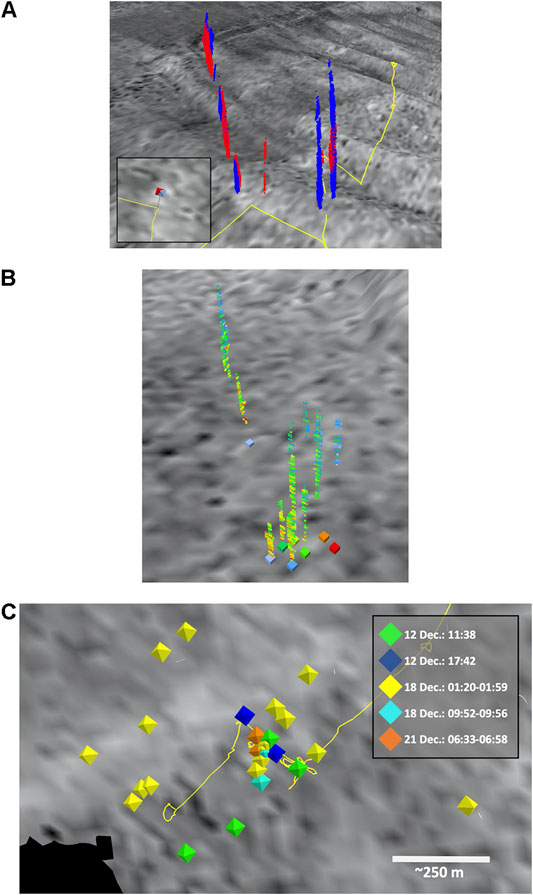
FIGURE 8. (A) Comparison of EM302 (blue) and EM710 (red) bubble plumes in SA1: Pacuare. Excellent overlap of points recorded at same time supports interpretation that both sonars imaging same plumes. Plumes on left side near sharp corner in ROV path (yellow line) are SC2. Inset figure shows seafloor source of S1 (blue) and S2 (red). Distance along yellow ROV path between the two seep clusters ∼450 m. (B) Moderate confidence anomalies identified on EM710, SA2: Savegre-SC3. No comparable anomalies are apparent on EM302 data, offering evidence of false negative in 30 kHz data. Colors in water column anomalies represent acoustic backscatter amplitude with red colors at +10 dB and light blue colors at −9 dB. Distance between main grouping of plumes and outlier plume ∼380 m (C) Time series of EM302 data, SA2: Savegre-SC2. While anomalies were observed at all times, number of anomalies varies over 9-days timespan.
The manner of multiple ship operations also provides a time record of bubble plumes with as many as five observations made over 9 days (Figure 8C). The details of this comparison are provided in Supplementary Material, but the complexities of varying seep flux, changing ocean current directions and magnitude, and uncertainty in seafloor source locations make comparison of specific seeps difficult to impossible. While a multitude of sonar issues (e.g., static offsets and ray-tracing errors) can affect the location of water column anomalies in space, we think the biggest potential error arises from the extrapolation of water column points, especially when the base is above the seafloor, back to its seafloor source. However, comparing seeps within a seep cluster is feasible (Figure 8C), and the spatial scale of clusters is comparable to the grid dimensions used by Spock (50 m), which minimizes the impact of small errors locating individual seeps. Within the 9- days observation period most seep clusters remain active although the number of individual seeps will change. There are seep clusters (e.g., SA3: Savegre—SC3; Figure 8B) that are only observed at one time (two observations).
Acoustic anomalies recorded by the AUG sonar provide a novel contribution to the time history of seeps. The AUG sonar recorded acoustic anomalies near anomalies documented by EM302 and EM710 data (Figure 5), but additional anomalies are identified farther from established anomalies. These may be false positive results, or they could reflect lower bubble fluxes or smaller bubble sizes-further research is required to work out the limits of this new approach. Nevertheless, the potential for an AUG sonar to document a long-term time record of seeps identified by ship-based sonars is tremendous.
Because this is a well-studied margin and our cruise revisited documented seep locations, our results contribute to the record of decade-scale seep durability. However, previous authors apply the term seeps at a multitude of scales so some translation of previous results into our seep/seep cluster/seep array hierarchy is required. Comparison of individual seeps at a scale of 2–5 m—well below mapping resolution—is difficult to impossible so a more feasible objective is comparison of seep clusters and seep arrays.
The crest of the Jaco scar was identified as a site of active seepage (Sahling et al., 2008), and our expedition recovered CTD samples with methane well above background at the same sites sampled by Mau et al. (2014). Some of the seep clusters within SA4: Jaco (SC3, 4, 7, 8 in Table 1) contain well-developed deep-sea corals that would have used seep-related carbonates as a substrate. There was limited evidence along our ROV dive paths, however, for bacterial mats or other fauna that require a continuous, currently active source of methane, and no water column acoustic anomalies were observed, suggesting that at least some of the seeps are dormant. However, our Jaco seep sites visited by ROV are different than those studied by Mau et al. (2014) so even though they documented seep evolution on the year timescale with subsequent cruises, we can only confirm that the Jaco seep array maintains evidence of seepage on a 15- years timescale.
Previous expeditions to Mounds 11 and 12 collected methane flux observations between 2002 and 2009 (Linke et al., 2005; Mau et al., 2006; Füri et al., 2010; Tryon et al., 2010; Levin et al., 2015). All expeditions observed elevated methane concentrations near the seafloor. In 2005, the R/V Atlantis (AT-11-28) deployed submarine flux meters for 12 months (Füri et al., 2010). High-flux events were observed near the beginning and end of the deployment, as well as in late Sept-early Oct 2005, approximately midway through the deployment (Füri et al., 2010). Füri et al. (2010) also noted episodic free gas expulsions at Mounds 11 and 12 in the Spring of 2009 (RV Atlantis AT 15–44). Combining our observations with these previous data leads to the recognition that the Mound 11 seep system (our SA3: SC4) remains active on the days, weeks, months, year-long, and 15- years timescales, and the adjacent Mound 11 seep cluster (SA3: SC3) visited by Tryon et al. (2010), where they observed mats, may have become dormant (Table 1). Comparing our results for Mound 12 with previous work is complicated by the fact that Tryon et al. (2010) report no location information for their observations, but both of the seep clusters that we observed (SA3: SC1 and SC2) had either ROV-observed bubbles or mats (Table 1), consistent with the record of mats by Tryon et al. (2010) at Mound 12 and the observation of seep biota on the seafloor and methane in seawater above Mound 12 by Mau et al. (2006). On this basis, we conclude that Mound 12 has remained an active seep for 13 years or more. U/Th dates of the seep-derived carbonate at the two sites range from 3.4 to 10 ka (Kutterolf et al., 2008), reflecting a protracted history of seep processes during which shorter period processes wax and wane.
All of the observations regarding short- and long-term seep episodicity and durability suggest that the search for active seeps is best conducted at the scale of seep clusters and arrays, with a search duration of at least 1–2 weeks. Autonomous approaches such as AUG water column mapping coupled to Spock’s decision-making capabilities constitute a possible breakthrough in our ability to identify and map these systems efficiently and at low-cost.
The goal of this study is to improve the chances of finding seeps with deep-sourced fluids using a Ladder of Seeps framework. Inorganic fluid chemistry is critical to this effort as a means of gaining insights into silicate mineral reactions in seismogenic intervals (e.g., Moore and Vrolijk, 1992). Because fluid volumes at seismogenic depths (ca. 10–15 km) are small compared to the fluid volume in near-surface, porous sediments, extreme dilution of deep fluids is expected for shallow samples. Organic gases serve as a deep-fluid proxy if compounds are discovered that only form at elevated temperatures.
The characteristics of deep-sourced fluids along the Costa Rican margin, defined by ODP Leg 170 and IODP Expedition 334 samples and analyses, include lower salinity fluids (e.g., Silver et al., 2000), Li and Ca enrichment (Chan and Kastner, 2000; Kopf et al., 2000; Torres et al., 2014; Expedition 334 Scientists, 2011) and elevated B (Kopf et al., 2000). In addition, higher hydrocarbons are found in active subduction faults (Lückge et al., 2002), and ethane is interpreted as coming from a thermogenic source based on carbon isotope ratios.
We applied three methods to seek deep-sourced fluids. Two methods (CTD water samples and in-situ mass spectrometry; Figure 2, top Ladder rung) search for dissolved hydrocarbon gases in the ocean that reflect deep-sourced fluids. The final method, samples from sediment cores, yields more detailed information on proxy gases and inorganic chemistry. The mass spectrometer deployed on the ROV produces a larger dataset (ca. 3100 samples vs. 16 sediment and two CTD water samples) collected while undergoing other tasks, and it allows qualitative identification of anomalies in real-time. Sediment and CTD water samples require dedicated ship time to collect and the technical experience to choose the ‘best’ sample locations, but they provide more detailed information about concentrations and isotopic ratios as well as inorganic species. The benefits and limitations of each method are outlined in Supplementary Table S7, but our synthesis suggests that a combination of approaches provides the greatest confidence in ascending the ladder to the top rung: confirmed deep-sourced fluids.
The inorganic geochemistry of pore waters offers no compelling evidence for deep-sourced fluids. While some measurements of Cl are below seawater values, as low as 524 mM/l, these values remain closer to seawater chlorinity than the values found in ODP drilling (Silver et al., 2000), and our samples’ proximity to hydrate makes Cl variations from hydrate formation/disassociation difficult to exclude. Li concentrations (Table 2) are lower than seawater concentrations, consistent with the observations of Torres et al. (2014), and the one sample with more Li than seawater is well below the Li concentration inferred to reflect deep fluid sources (74 μM; Torres et al., 2014 and up to 148 μM, Kopf et al., 2000). Measured calcium concentrations are likely primarily affected by abundant carbonate crust formation, and indeed most values are below seawater concentration (Table 3). While some samples have B concentrations above seawater, these are interpreted as resulting from alteration of organic matter (see below).
Methane is one species that is found in high concentrations with respect to seawater. In Figure 9A, samples are divided into those with <1 mM concentration (blue border), 1–10 mM (orange border), and >10 mM (red border). Samples with no methane have near-seawater sulfate concentrations. In many methane-rich samples, sulfate is almost exhausted. Samples without methane have >2× B than seawater (Figure 9B), much more P than seawater (Figure 9C), and near-seawater Ca concentrations (Figure 9D). This pattern of concentrations is interpreted as alteration of organic matter contributing B and P species to porewaters without any calcite precipitation.
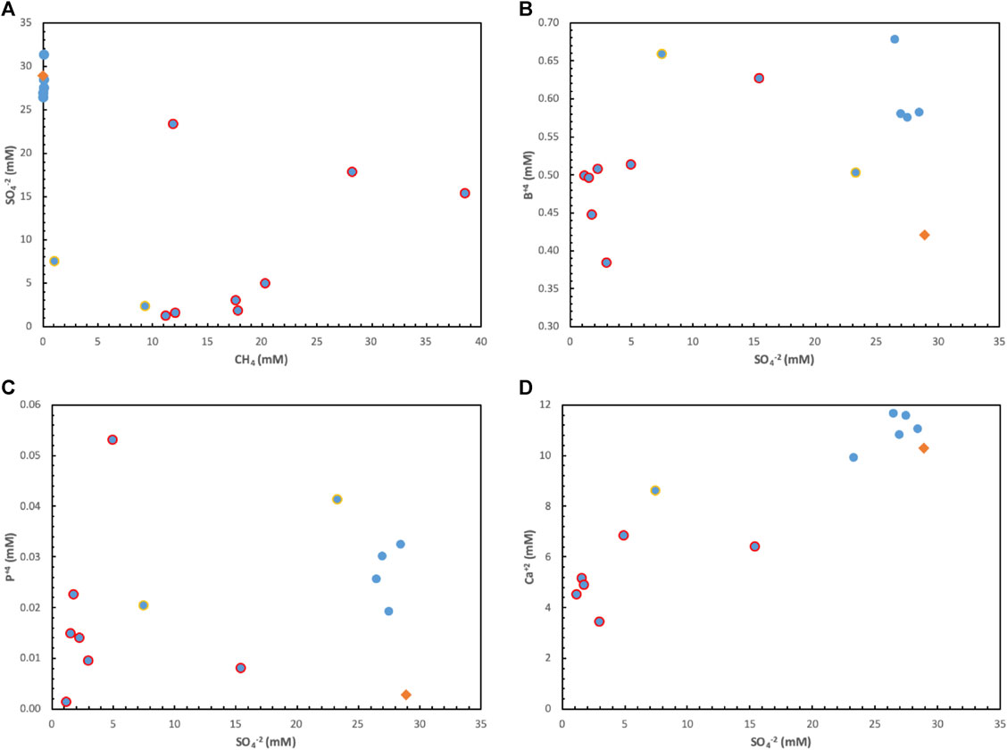
FIGURE 9. Pore water summary graphs for methane alteration processes. In each plot orange diamond is seawater reference. Samples with >10 mM methane outlined in red, and 1–10 mM methane outlined in orange. Methane-poor samples (<1 mM) have no outline. (A) Head-space methane gas concentration vs. pore water sulfate concentration. Many methane-rich samples are depleted in sulfate. (B) Sulfate vs. boron concentration in pore waters. Methane-poor samples enriched in B with respect to seawater, reflecting organic matter degradation without sulfate reduction. Most methane-rich samples have B concentrations closer to seawater. (C) Sulfate vs. phosphorous concentration in pore waters. Methane-poor samples enriched in P with respect to seawater, reflecting organic matter degradation without sulfate reduction. Most methane-rich samples have P concentrations closer to seawater, but 2 methane-rich samples have high P concentration. (D) Sulfate vs. calcium concentration in pore waters. Methane-poor samples have sulfate and Ca concentrations near seawater but methane-rich samples have depleted sulfate and Ca from carbonate precipitation.
In contrast, the methane-rich samples have B and P concentrations much closer to seawater values, and calcium concentrations are half or less than seawater concentrations. For these samples the source of carbon is methane, which is consumed by Anaerobic Oxidation of Methane (AOM; e.g., Milucka et al., 2012), which results in no change in B or P concentrations. AOM reactions consume sulfate (Milucka et al., 2012), resulting in the near exhaustion of sulfate in methane-rich samples.
Carbon isotope ratios of methane show no clear pattern with methane concentration (Figure 7) but range from values around −50‰ that could reflect thermogenic methane and values as low as −84.6‰, which represent biogenic methane. Interpretation of thermogenic methane at Mound 11 (Figure 7) is consistent with more detailed analyses, as is the biogenic gas interpretation for Mound 12 (Schmidt et al., 2005; Füri et al., 2010; Krause et al., 2014).
In headspace gas samples, ethane, propane, and benzene are detected (Table 3), but the gas concentrations remain unquantified. Propane and benzene occurrences are especially critical because there is a high probability that they are only produced by thermal cracking of organic matter. Moreover, in-situ mass spectrometer measurements (Figure 10) indicate propane and benzene anomalies at just over half of the seep clusters visited, and in just over half of those sites they occur together. Even though carbon isotope ratios of methane samples indicate a large biogenic gas component in many samples, the presence of propane and benzene in samples suggests that seeps at all dive sites have some unquantified fraction of thermogenic gas.
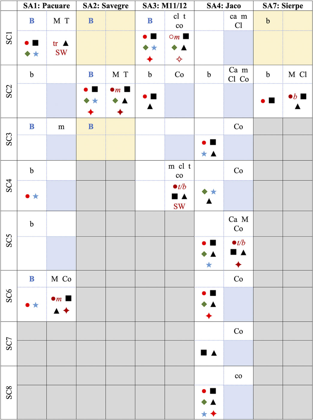
FIGURE 10. Synthesis of seep results. Data arranged by seep array (columns) and cluster (rows); gray boxes indicate no seep cluster defined, orange boxes reflect seep clusters unvisited by ROV, and blue boxes visited by ROV but no samples obtained. Each seep cluster divided into 4 observation types: 1) acoustic anomalies/bubble plumes (upper left); B: 5 + plumes, b: <5 plumes, and blank = 0 plumes; 2) observed seep biota and substrate (upper right) where upper case indicates major component and lower case is minor component; M: mats; T: tubeworms; Cl: clams; Co: corals; Ca: carbonate; 3) mass spectrometer anomalies (lower left); ●: methane; ethane; ◆: propane; ▲: benzene; ★: carbon dioxide; ✦: hydrogen sulfide); 4) pore water and head-space gas results from push cores (lower right); ●: methane >20 mM; ○: methane = 1–10 mM; tr: methane <0.1 mM; ethane; ◆: propane; ▲: benzene; ✦: sulfate = 0–5 mM; ✧: sulfate = 2–20 mM; SW: sulfate = >20 mM; letters following methane symbols indicate δ13C ratios: t: -40 to −50‰; m: −50 to −65‰; b: < −65‰.
While it is tempting to try to work out biogenic/thermogenic gas proportions based on carbon isotope ratios, the problem is further complicated by AOM processes that can increase the carbon isotopic value of residual methane if methane conversion is incomplete (e.g., Whiticar, 1999). Sulfate concentrations in pore water combined with flux inferences derived from seep biota (e.g., mats reflect high fluxes) could constrain AOM reaction progress, a necessary variable in the Rayleigh distillation problem arising from incomplete AOM consumption. Preliminary calculations suggest that our data suite remains too unconstrained to provide meaningful estimates of thermogenic gas proportion.
In summary, hydrocarbon gases offer good evidence for deep-sourced fluids, and on this basis, we confirm access to a deep fluid source at Mound 11 and suggest that most or all sites have received some component of thermogenic gas. While AOM complicates interpretation of a thermogenic gas from carbon isotope ratios, the presence of propane and benzene are proxy indicators of a thermogenic gas component. If Spock were expanded to rank the probability of sampling a higher concentration of deep-sourced fluids in subsurface samples (e.g., by scientific drilling) at each seep cluster, then an evolved approach that yields an improved estimate of the fraction of thermogenic gas is warranted.
Formal decision-support systems offer a number of benefits for documenting important decisions undertaken during scientific investigations and rendering them reproducible. These systems require a clear definition of what constitutes advancement and success, and the Ladder of Seeps was developed as a foundation for this purpose. A crucial aspect of decision-support systems is that they tolerate analytical uncertainty that may arise from processing and interpreting data quickly if that uncertainty has no appreciable impact on the probability distributions used by Spock. In other words, the use of a decision-support system specifies where back-of-the-envelope results are sufficient, and where results must be produced at a high precision. All of the data collection and analysis efforts in our study follow this principle (e.g., construction of a seafloor backscatter product using a generic processing workflow).
As deployed on this expedition, Spock was intended to improve the probability that visited sites could ascend to the ‘Seep’ rung in the Ladder of Seeps. Conceptually, this is performed by analyzing remote observations that allow a site to be identified as ‘Possible Seep’ or ‘Likely Seep’, and identifying combinations of observations that are more likely to be associated with fluid release. Because photographic identification is used to identify seep-dependent biota and confirm the acoustic bubble plume interpretation by verifying the flux of nutrients to the seafloor, visiting the site remains necessary to move up the ladder. Spock allows the associations between combinations of features and seepage probability to be learned quickly and balances the advantage of gathering new information against the benefits of visiting sites with high probability of seepage. Using Spock to perform dive planning resulted in significant time savings, allowed dives to make use of information from the most recent observations, and generated an objective record of why specific sites were chosen for investigation. A more detailed comparison between Spock and human-planned dives in terms of time and efficacy is presented in the Supplementary Material.
Even though our survey area was large and many seeps were visited, the number of unique observations remains small (Table 4), leading to some counter-intuitive conclusions. For example, the inference that high slope areas (normal fault scarps) are a good indicator that no seeps will be found (Table 5) arises from the Spock search for active seeps. Normal fault scarps are most common over the Jaco Scar, but the absence of water column anomalies and the abundance of deep-sea corals led us to consider this a dormant and weak-active (SA4: Jaco—SC5) seep array. The in-situ mass spectrometer data recorded a large number of anomalies for all species (Figure 10), but we think the number of anomalies is more affected by local data acquisition conditions than seep flux. How seeps are classified is critical for Spock’s success, and this is an area that requires further research to reach a scientific consensus, which in turn will lead to modifications of the Ladder of Seeps. The Ladder is an explicit description of a community picture of seep systems. The Spock algorithms will benefit from a database of priors that incorporates more global information about seeps at different scales while retaining the flexibility to adapt to local conditions. Moreover, the means to steer vehicles away from sites that have features without demonstrated seepage is an important benefit that probably exceeds human capabilities.
As an example, Spock inferred that mounds are considered good indicators that no seeps will be found. However, this inference arises because features are defined at a scale of 50 m, a dimension chosen to ensure a high probability of finding a seep at that location if there is one to be found. Others have described mounds as an important seep element in this region, but those descriptions are at the scale of a seep cluster (e.g., Klaucke et al., 2008, describe Mounds 11 and 12 as 600–1000 m across) that is too large for efficient seep surveys. Bathymetric morphologies defined at a multitude of scales may further help identify successful seep candidates. The observation also illustrates the importance of adding water column data to Spock’s priors-high predicted probabilities for Dive nine sites (with no mound) depended on the availability of preliminary water column processing.
The Spock algorithms used observations from MBES and ROV dives to improve the planning and prediction model, resulting in shifts in the relative importance of different features (Table 5). The rate-limiting step in this work was the processing of raw MBES data and preliminary interpretation. Even simple tasks like identifying bathymetric morphology are daunting with large datasets, in particular if considering morphologic features at multiple scales of observation. Efficient, automated systems for aiding this analysis are available (e.g., Geomorphons; Jasiewicz and Stepinski, 2013) and could be added to the workflows. The presence of water column anomalies had the biggest impact on the success of finding seeps, but it was impossible to process the water column data during the cruise with the limited staff available. While the Feature Detection filters in FMMidwater are a benefit for finding anomalies, either more staff or faster filtering methods are needed to produce precise seafloor seep locations for Spock predictions in real-time.
The combined Ladder of Seeps and Spock approach could be modified to address other pressing questions, like estimating global fluxes of chemical species from seeps (e.g., Mau et al., 2006). Improved estimates probably derive from recognizing different seep types with different time-integrated fluxes. An analogous Ladder could be constructed to help define these seep types and the data needed to confirm any particular seeps as one type at a specified confidence level, and a Spock routine could be devised to efficiently collect the necessary data to achieve a confident extrapolation to all seep candidates.
To address the question posed at the outset, the combined Ladder of Seeps and Spock approach provided us an effective and inexpensive means to identify seeps with the potential to yield deep-sourced fluids. Thirty seep sites were identified and visited with 9 ROV dives over the space of only 10 days, facilitated by the application of the Ladder framework within Spock’s decision-making algorithms, coupled to historical data. High resolution bathymetry and backscatter data, coupled with water column anomalies allowed us to get from Possible to Likely Seep and helped us identify successful targets for ROV dives that collected observations allowing us to ascend to the highest confirmed seep rungs.
As a result of this short expedition, we identify SA3: Mound 11 and SA1: Pacuare as good candidates to pursue subsurface data collection studies to evaluate fluid migration pathways that could be sampled via cores taken hundreds of meters below the seafloor to obtain undiluted samples of deep-sourced fluids. A fair question is whether Spock would have brought us to Mound 11 in the absence of prior seep information and the absence of bubbles, but the proximity to Mound 12, the bathymetric morphology, and the high backscatter may have sufficed. In contrast, the decision to visit SA1: Pacuare was solely Spock’s and is predicated based on the high number of bubble plumes, the close proximity of seep targets, and the bathymetric morphology and backscatter character. There is no prior indication of seeps at SA1: Pacuare. Seismic imaging of potential deep fluid-flow pathways at these seep clusters would reinforce the screening data collected during this study and provide a compelling reason for scientific drilling likely to result in a high probability of scientific success. Crutchley et al. (2014), in their study of the impact of fluid advection on gas hydrate stability at Mounds 11 and 12, used 2D and 3D seismic data to illustrate possible fault-related fluid-flow pathways for the gas in hydrates at those seep sites. A similar approach could be taken for SA1: Pacuare.
The use of Spock in this expedition contributed objectivity, repeatability, and time savings to the process of dive planning. Scoring all sites ensured that promising locations were not overlooked, while continuous data assimilation meant that sites were reconsidered under the most up-to-date understanding of the environment. Further, the algorithms provided a means to optimize probability of finding seepage against constraints on ROV dive time. This optimization was performed several hours faster than an equivalent dive could have been hand-designed and allowed the science team to focus instead on data interpretation.
From a broader perspective, our use of Spock also represents a step forward in the application of automated reasoning to intelligent exploration of the oceans and planetary bodies. Autonomous exploration vehicles must be able to learn from data and reason about the priorities of observations. Spock demonstrated this capability through the prediction of seep likelihoods and selection of dive sites to maximize probability of climbing the Ladder of Seeps. Deployment of such a system would lead to more thorough examination over a longer duration than has previously been possible, without the need for frequent communication and the risk and expense of manned exploration, or the need for frequent communication with remotely operated systems.
Our research expedition set out to apply and test new analytical and decision-support systems in the search for cold seeps in the Costa Rican accretionary margin. Existing seep locations were visited to confirm the viability of our systems against existing knowledge, but additional seep locations were also discovered with our methods. A Ladder of Seeps was developed in the context of a specific scientific goal-identify seep sites with deep-sourced fluids-and it served as a foundation for Spock, which was used in ROV and AUG dive planning to collect additional data to further ascend the ladder. Many of the new seep sites discovered are attributed to MBES water column imaging methods, but the use of AUG sonar to identify water column anomalies shows the potential to collect additional information without the use of a dedicated surface ship. Data from an in-situ mass spectrometer deployed on the ROV complements data collected from traditional sediment sample methods. We think that the use of advanced data collection and decision-support technologies will elevate our understanding of how cold seep systems contribute to Earth systems.
The datasets generated for this study can be found in the R2R repository (https://www.rvdata.us/data).
RC was chief scientist for the R/V Falkor cruise, contributed processing and analysis of AUG sonar data, operated and processed in-situ mass spectrometer data, and led coordination of the diverse disciplinary tasks. PV, LS, and PN guided ROV dives and recorded observations, directed and processed samples on the ship, and interpreted new MBES bathymetry and backscatter data. PV processed water column data on the ship and post-cruise and took lead responsibility for writing this manuscript. LS compiled and integrated bathymetry, backscatter, bubble plume source, and Squidle+ data into maps and described those processes and results in this manuscript. BA executed missionplanning algorithms (Spock) on the ship and wrote up those processes and results here. AH collaborated on pore water chemistry analyses, FK measured methane concentrations in headspace gas and CTD water samples, and DV provided the laboratory resources for methane concentration analyses. SS contributed carbon isotope ratio measurements of methane from headspace gas samples.
Support for this research was provided through NASA PSTAR Grant #NNX16AL08G and National Science Foundation Navigating the New Arctic grant #1839063. Use of the R/V Falkor and ROV SuBastian were provided through a grant from the Schmidt Ocean Institute. The AUG Nemesis and the Aurora in-situ mass spectrometer was provided through in-kind support from Teledyne Webb Research and Navistry Corp, respectively.
The authors declare that the research was conducted in the absence of any commercial or financial relationships that could be construed as a potential conflict of interest.
The authors wish to thank NASA, the National Science Foundation, Schmidt Ocean Institute, Teledyne Webb Research, and Navistry Corp for their generous support, as well as the country of Costa Rica for permitting operations in national waters. Additionally, the authors would like to recognize the valuable contributions of the entire FK181210 science team and especially Angelos Mallios and David Pingal for AUG support, Eric Timmons for computational support, and Ariell Friedman for Squidle + modifications and support. Bathymetry and acoustic backscatter maps were created by Marine Tech Deborah Smith (Schmidt Ocean Institute) and delivered to the scientific party as input to the seep-hunting analysis. Finally, the authors would like to thank the captain and crew of the R/V Falkor as well as the ROV SuBastian operations team for their skillful and friendly assistance.
The Supplementary Material for this article can be found online at: https://www.frontiersin.org/articles/10.3389/feart.2021.601019/full#supplementary-material
Data Sheet 1 | Seep_Array_Documentation.pdf
Data Sheet 2 | Supplementary Files (Annotations-ROV Excel files)
Data Sheet 3 | Supplementary Text
Data Sheet 4 | Supplementary Tables 1-9
Image 1 | Supplementary Figure 1
1https://schmidtocean.org/technology/robotic-platforms/4500-m-remotely-operated-vehicle-rov/
4https://confluence.qps.nl/fledermaus7/how-to-articles/how-to-fmmw/how-to-fmmidwater-feature-detection-in-fmmidwater
Anderson, V. C. (1950). Sound scattering from a fluid sphere. J. Acoust. Soc. Am. 22 (4), 426–431. doi:10.1121/1.1906621
Barnes, P. M., Lamarche, G., Bialas, J., Henrys, S., Pecher, I., Netzeband, G. L., et al. (2010). Tectonic and geological framework for gas hydrates and cold seeps on the Hikurangi subduction margin, New Zealand. Mar. Geol. 272 (1–4), 26–48. doi:10.1016/j.margeo.2009.03.012
Barth, J. A., and Chafetz, H. S. (2015). Cool water geyser travertine: crystal geyser, utah, united states. Sedimentology 62 (3), 607–620. doi:10.1111/sed.12158
Baumberger, T., Embley, R. W., Merle, S. G., Lilley, M. D., Raineault, N. A., and Lupton, J. E. (2018). Mantle‐derived helium and multiple methane sources in gas bubbles of cold seeps along the cascadia continental margin. Geochem. Geophys. Geosyst. 19 (11), 4476–4486. doi:10.1029/2018gc007859
Bohrmann, G., Heeschen, K., Jung, C., Weinrebe, W., Baranov, B., Cailleau, B., et al. (2002). Widespread fluid expulsion along the seafloor of the Costa Rica convergent margin. Terra Nova 14 (2), 69–79. doi:10.1046/j.1365-3121.2002.00400.x
Bowden, D. A., Rowden, A. A., Thurber, A. R., Baco, A. R., Levin, L. A., and Smith, C. R. (2013). Cold seep epifaunal communities on the Hikurangi Margin, New Zealand: composition, succession, and vulnerability to human activities. PLoS One 8 (10), e76869, doi:10.1371/journal.pone.0076869
Buntine, W. L. (1994). Operations for learning with graphical models. JAIR 2, 159–225. doi:10.1613/jair.62
Camilli, R., Bingham, B., Reddy, C. M., Nelson, R. K., and Duryea, A. N. (2009). Method for rapid localization of seafloor petroleum contamination using concurrent mass spectrometry and acoustic positioning. Mar. Pollut. Bull. 58 (10), 1505–1513. doi:10.1016/j.marpolbul.2009.05.016
Camilli, R., Reddy, C. M., Yoerger, D. R., Van Mooy, B. A., Jakuba, M. V., Kinsey, J. C., et al. (2010). Tracking hydrocarbon plume transport and biodegradation at deepwater horizon. Science 330 (6001), 201–204. doi:10.1126/science.1195223
Campbell, K. A., Farmer, J. D., and Des Marais, D. (2002). Ancient hydrocarbon seeps from the Mesozoic convergent margin of California: carbonate geochemistry, fluids and palaeoenvironments. Geofluids 2 (2), 63–94. doi:10.1046/j.1468-8123.2002.00022.x
Chan, L. H., and Kastner, M. (2000). Lithium isotopic compositions of pore fluids and sediments in the Costa Rica subduction zone: implications for fluid processes and sediment contribution to the arc volcanoes. Earth Planet. Sci. Lett. 183 (1, 2), 275–290. doi:10.1016/s0012-821x(00)00275-2
Cordes, E. E., McGinley, M. P., Podowski, E. L., Becker, E. L., Lessard-Pilon, S., Viada, S. T., et al. (2008). Coral communities of the deep Gulf of Mexico. Deep Sea Res. Oceanogr. Res. Pap. 55 (6), 777–787. doi:10.1016/j.dsr.2008.03.005
Crutchley, G. J., Klaeschen, D., Planert, L., Bialas, J., Berndt, C., Papenberg, C., et al. (2014). The impact of fluid advection on gas hydrate stability: Investigations at sites of methane seepage offshore Costa Rica. Earth Planetary Sci Lett. 401, 95–109. doi:10.1016/j.epsl.2014.05.045
Desrosiers, J., Dumas, Y., Solomon, M. M., and Soumis, F. (1995). Chapter 2 Time constrained routing and scheduling. Handbooks Operat. Res. Manag. Sci. 8, 35–139. doi:10.1016/s0927-0507(05)80106-9
Dickens, G. R., and Quinby-Hunt, M. S. (1994). Methane hydrate stability in seawater. Geophys. Res. Lett. 21 (19), 2115–2118. doi:10.1029/94gl01858
Duguid, Z., and Camilli, R. (2020). Improving resource management for unattended observation of the marginal ice zone using autonomous underwater gliders. Front. Robot. AI 7, 579256. doi:10.3389/frobt.2020.579256
Expedition 334 Scientists, (2011). Costa Rica Seismogenesis Project (CRISP): sampling and quantifying input to the seismogenic zone and fluid output. IODP Prel. Rept. 334, 114. doi:10.2204/iodp.pr.334.2011
Feseker, T., Boetius, A., Wenzhöfer, F., Blandin, J., Olu, K., Yoerger, D. R., et al. (2014). Eruption of a deep-sea mud volcano triggers rapid sediment movement. Nat. Commun. 5 (1), 5385–5388. doi:10.1038/ncomms6385
Füri, E., Hilton, D. R., Tryon, M. D., Brown, K. M., McMurtry, G. M., Brückmann, W., et al. (2010). Carbon release from submarine seeps at the Costa Rica fore arc: implications for the volatile cycle at the Central America convergent margin. Geochem. Geophys. Geosyst. 11 (4). doi:10.1029/2009gc002810
Gaschnig, J. (1982). in Prospector: an expert system for mineral exploration. Editor D. Michie, 47–64. New York: Gordon and Breach Science Publishers.
Gomes-Pereira, J. N., Auger, V., Beisiegel, K., Benjamin, R., Bergmann, M., Bowden, D., et al. (2016). Current and future trends in marine image annotation software. Prog. Oceanogr. 149, 106–120. doi:10.1016/j.pocean.2016.07.005
Gouveia, F. J., and Friedmann, S. J. (2006). Timing and prediction of CO2 eruptions from Crystal Geyser, UT (No. UCRL-TR-221731). Livermore, CA (United States): Lawrence Livermore National Lab.(LLNL).
Grant, N. J., and Whiticar, M. J. (2002). Stable carbon isotopic evidence for methane oxidation in plumes above Hydrate Ridge, cascadia oregon margin. Glob. Biogeochem. Cycles 16 (4), 71–1. doi:10.1029/2001GB001851
Guillon, E., Menot, L., Decker, C., Krylova, E., and Olu, K. (2017). The vesicomyid bivalve habitat at cold seeps supports heterogeneous and dynamic macrofaunal assemblages. Deep Sea Res. Part Oceanogr. Res. Pap. 120, 1–13. doi:10.1016/j.dsr.2016.12.008
Hand, K. P., and German, C. R. (2018). Exploring ocean worlds on Earth and beyond. Nat. Geosci. 11 (1), 2–4. doi:10.1038/s41561-017-0045-9
Hensen, C., Wallmann, K., Schmidt, M., Ranero, C. R., and Suess, E. (2004). Fluid expulsion related to mud extrusion off Costa Rica-A window to the subducting slab. Geology 32 (3), 201–204. doi:10.1130/g20119.1
Jasiewicz, J., and Stepinski, T. F. (2013). Geomorphons - a pattern recognition approach to classification and mapping of landforms. Geomorphology 182, 147–156. doi:10.1016/j.geomorph.2012.11.005
Judd, A. G. (2004). Natural seabed gas seeps as sources of atmospheric methane. Environ. Geol. 46 (8), 988–996. doi:10.1007/s00254-004-1083-3
Judd, A., and Hovland, M. (2009). Seabed fluid flow: the impact on geology, biology and the marine environment. Cambridge: Cambridge University Press. doi:10.1017/CBO9780511535918
Kastner, M., Elderfield, H., and Martin, J. B. (1991). Fluids in convergent margins: what do we know about their composition, origin, role in diagenesis and importance for oceanic chemical fluxes?. Philos. Trans. R. Soc. Lond. Ser. A Phys. Eng. Sci. 335 (1638), 243–259. doi:10.1098/rsta.1991.0045
Kaufmann, E., Cappe, O., and Garivier, A. (2012). On Bayesian Upper Confidence Bounds for Bandit Problems, in: Proceedings of the fifteenth international conference on artificial intelligence and statistics La Palma, Canary Islands: MLResearchPress, in PMLR 22:592-600.
Klaucke, I., Masson, D. G., Petersen, C. J., Weinrebe, W., and Ranero, C. R. (2008). Multifrequency geoacoustic imaging of fluid escape structures offshore Costa Rica: implications for the quantification of seep processes. Geochem. Geophys. Geosyst. 9 (4), 708. doi:10.1029/2007gc001708
Kluesner, J. W., Silver, E. A., Bangs, N. L., McIntosh, K. D., Gibson, J., Orange, D., et al. (2013). High density of structurally controlled, shallow to deep water fluid seep indicators imaged offshore costa rica. Geochem. Geophys. Geosyst. 14 (3), 519–539. doi:10.1002/ggge.20058
Kopf, A., Deyhle, A., and Zuleger, E. (2000). Evidence for deep fluid circulation and gas hydrate dissociation using boron and boron isotopes of pore fluids in forearc sediments from costa rica (ODP Leg 170). Mar. Geology 167 (1, 2), 1–28. doi:10.1016/s0025-3227(00)00026-8
Krause, S., Steeb, P., Hensen, C., Liebetrau, V., Dale, A. W., Nuzzo, M., et al. (2014). Microbial activity and carbonate isotope signatures as a tool for identification of spatial differences in methane advection: a case study at the Pacific Costa Rican margin. Biogeosciences 11, 507–523. doi:10.5194/bg-11-507-2014
Kutterolf, S., Liebetrau, V., Mörz, T., Freundt, A., Hammerich, T., and Garbe-Schönberg, D. (2008). Lifetime and cyclicity of fluid venting at forearc mound structures determined by tephrostratigraphy and radiometric dating of authigenic carbonates. Geology 36 (9), 707–710. doi:10.1130/g24806a.1
Lattimore, T., and Szepesvári, C. (2020). Bayesian bandits. Bandit algorithms. Cambridge: Cambridge University Press, 438–457.
Leifer, I., Luyendyk, B. P., Boles, J., and Clark, J. F. (2006). Natural marine seepage blowout: contribution to atmospheric methane. Glob. Biogeochem. Cycles 20 (3), 268. doi:10.1029/2005gb002668
Lessard-Pilon, S., Porter, M. D., Cordes, E. E., MacDonald, I., and Fisher, C. R. (2010). Community composition and temporal change at deep Gulf of Mexico cold seeps. Deep Sea Res. Part Topical Stud. Oceanogr. 57 (21–23), 1891–1903. doi:10.1016/j.dsr2.2010.05.012
Levin, L. A., Mendoza, G. F., Grupe, B. M., Gonzalez, J. P., Jellison, B., Rouse, G., et al. (2015). Biodiversity on the rocks: macrofauna inhabiting authigenic carbonate at Costa Rica methane seeps. PLoS One 10 (7), e0131080. doi:10.1371/journal.pone.0131080
Levin, L. (2005). Ecology of cold seep sediments. Oceanogr. Mar. Biol. Annu. Rev. 43, 1–46. doi:10.1201/9781420037449.ch1
Lindsay, R. K., Buchanan, B. G., Feigenbaum, E. A., and Lederberg, J. (1993). DENDRAL: a case study of the first expert system for scientific hypothesis formation. Artif. Intell. 61 (2), 209–261. doi:10.1016/0004-3702(93)90068-m
Linke, P., Wallmann, K., Suess, E., Hensen, C., and Rehder, G. (2005). In situ benthic fluxes from an intermittently active mud volcano at the Costa Rica convergent margin. Earth Planet. Sci. Lett. 235 (1, 2), 79–95. doi:10.1016/j.epsl.2005.03.009
Lückge, A., Kastner, M., Littke, R., and Cramer, B. (2002). Hydrocarbon gas in the Costa Rica subduction zone: primary composition and post-genetic alteration. Org. Geochem. 33 (8), 933–943. doi:10.1016/s0146-6380(02)00063-3
MacKay, D. J. (1998). Introduction to Monte Carlo methods. Learning in graphical models. Dordrecht: Springer, 175–204. doi:10.1007/978-94-011-5014-9_7
Mau, S., Rehder, G., Arroyo, I. G., Gossler, J., and Suess, E. (2007). Indications of a link between seismotectonics and CH4 release from seeps off costa rica. Geochem. Geophys. Geosystems 8 (4). doi:10.1029/2006gc001326
Mau, S., Rehder, G., Sahling, H., Schleicher, T., and Linke, P. (2014). Seepage of methane at Jaco Scar, a slide caused by seamount subduction offshore costa rica. Int. J. Earth Sci. (Geol Rundsch) 103 (7), 1801–1815. doi:10.1007/s00531-012-0822-z
Mau, S., Sahling, H., Rehder, G., Suess, E., Linke, P., and Söding, E. (2006). Estimates of methane output from mud extrusions at the erosive convergent margin off costa rica. Mar. Geol. 225 (1–4), 129–144. doi:10.1016/j.margeo.2005.09.007
Medwin, H., and Clay, C. S. (1998). Fundamentals of acoustical oceanography, California. Academic Press. doi:10.1121/1.426950
Milucka, J., Ferdelman, T. G., Polerecky, L., Franzke, D., Wegener, G., Schmid, M., et al. (2012). Zero-valent sulphur is a key intermediate in marine methane oxidation. Nature 491 (7425), 541–546. doi:10.1038/nature11656
Mitchell, G. A., Orange, D. L., Gharib, J. J., and Kennedy, P. (2018). Improved detection and mapping of deepwater hydrocarbon seeps: optimizing multibeam echosounder seafloor backscatter acquisition and processing techniques. Mar. Geophys. Res. 39 (1, 2), 323–347. doi:10.1007/s11001-018-9345-8
Moore, J. C., and Vrolijk, P. (1992). Fluids in accretionary prisms. Rev. Geophys. 30 (2), 113–135. doi:10.1029/92rg00201
Neveu, M., Hays, L. E., Voytek, M. A., New, M. H., and Schulte, M. D. (2018). The ladder of life detection. Astrobiology 18 (11), 1375–1402. doi:10.1089/ast.2017.1773
Nikolopoulos, C. (1997). Expert systems: introduction to first and second generation and hybrid knowledge based systems, London: Marcel Dekker.
Peacock, S. A. (1990). Fluid processes in subduction zones. Science 248 (4953), 329–337. doi:10.1126/science.248.4953.329
Proctor, R., Langlois, T., Friedman, A., Mancini, S., Hoenner, X., and Davey, B. (2018). “Cloud-based national on-line services to annotate and analyse underwater imagery”, in IMDIS 2018 International Conference on Marine Data and Information Systems, 05-07 November 2018, Barcelona, Spain. 59, 49. Available at: https://imdis.seadatanet.org/content/download/121493/file/IMDIS2018_Proceedings.pdf.
Ranero, C. R., Grevemeyer, I., Sahling, H., Barckhausen, U., Hensen, C., Wallmann, K., et al. (2008). Hydrogeological system of erosional convergent margins and its influence on tectonics and interplate seismogenesis. Geochem. Geophys. Geosyst. 9 (3), 679. doi:10.1029/2007gc001679
Ranero, C. R., Weinrebe, W., Grevemeyer, I., Phipps Morgan, J., Vannucchi, P., and von Huene, R. (2003). Tectonic structure of the Middle America pacific margin and incoming cocos plate from Costa Rica to Guatemala, America. AGUFM, T52C–T0289.
Riedinger, N., Torres, M. E., Screaton, E., Solomon, E. A., Kutterolf, S., Schindlbeck‐Belo, J., et al. (2019). Interplay of subduction tectonics, sedimentation, and carbon cycling. Geochem. Geophys. Geosyst. 20 (11), 4939–4955. doi:10.1029/2019gc008613
Russo, D., and Van Roy, B. (2018). Learning to optimize via information-directed sampling. Operat. Res. 66 (1), 230–252. doi:10.1287/opre.2017.1663
Sahling, H., Galkin, S. V., Salyuk, A., Greinert, J., Foerstel, H., Piepenburg, D., et al. (2003). Depth-related structure and ecological significance of cold-seep communities-a case study from the Sea of okhotsk. Deep Sea Res. Part Oceanogr. Res. Pap. 50 (12), 1391–1409. doi:10.1016/j.dsr.2003.08.004
Sahling, H., Masson, D. G., Ranero, C. R., Hühnerbach, V., Weinrebe, W., Klaucke, I., et al. (2008). Fluid seepage at the continental margin offshore Costa Rica and southern nicaragua. Geochem. Geophys. Geosystems 9 (5), 978. doi:10.1029/2008gc001978
Schmidt, M., Hensen, C., Mörz, T., Müller, C., Grevemeyer, I., Wallmann, K., et al. (2005). Methane hydrate accumulation in “Mound 11” mud volcano, Costa Rica forearc. Mar. Geology 216 (1, 2), 83–100. doi:10.1016/j.margeo.2005.01.001
Sibuet, M., and Olu, K. (1998). Biogeography, biodiversity and fluid dependence of deep-sea cold-seep communities at active and passive margins. Deep Sea Res. Part Topical Stud. Oceanogr. 45 (1), 517–567. doi:10.1016/s0967-0645(97)00074-x
Silver, E., Kastner, M., Fisher, A., Morris, J., McIntosh, K., and Saffer, D. (2000). Fluid flow paths in the Middle America Trench and Costa Rica margin. Geology 28 (8), 679–682. doi:10.1130/0091-7613(2000)28<679:FFPITM>2.0.CO;2
Skarke, A., Ruppel, C., Kodis, M., Brothers, D., and Lobecker, E. (2014). Widespread methane leakage from the sea floor on the northern US Atlantic margin. Nat. Geosci. 7 (9), 657–661. doi:10.1038/ngeo2232
Suess, E. (2018). in Marine cold seeps: background and recent advances. Hydrocarbons, Oils and lipids: diversity, origin, Chemistry and fate. Editor H. Wilkes (Cham: Springer International Publishing), 1–21.
Sullivan-Silva, K. B. (1989). Underwater acoustic scattering from spherical particulates and bubbles. London, Connecticut: Naval Underwater Systems Center Newport RI.
Torres, M. E., Embley, R. W., Merle, S. G., Trehu, A. M., Collier, R. W., Suess, E., et al. (2009). Methane sources feeding cold seeps on the shelf and upper continental slope off central Oregon, USA. Geochem. Geophys. Geosyst. 10 (11). doi:10.1029/2009gc002518
Torres, M. E., Muratli, J. M., and Solomon, E. A. (2014). “Data report: minor element concentrations in pore fluids from the CRISP-A transect drilled during Expedition 334,” in The expedition 334 scientists, proc. IODP. Editors P. Vannucchi, K. Ujiie, N. Stroncik, and A. Malinverno (Tokyo: Integrated Ocean Drilling Program Management International, Inc.), 334. doi:10.2204/iodp.proc.334.201.2014
Tryon, M. D., Brown, K. M., and Torres, M. E. (2002). Fluid and chemical flux in and out of sediments hosting methane hydrate deposits on Hydrate Ridge, OR, II: H.ydrological processes. Earth Planet. Sci. Lett. 201 (3, 4), 541–557. doi:10.1016/s0012-821x(02)00732-x
Tryon, M. D., Brown, K. M., Torres, M. E., Tréhu, A. M., McManus, J., and Collier, R. W. (1999). Measurements of transience and downward fluid flow near episodic methane gas vents, hydrate ridge, cascadia. Geology 27 (12), 1075–1078. doi:10.1130/0091-7613(1999)027<1075:MOTADF>2.3.CO;2
Tryon, M. D., Wheat, C. G., and Hilton, D. R. (2010). Fluid sources and pathways of the Costa Rica erosional convergent margin. Geochem. Geophys. Geosyst. 11 (4), 818. doi:10.1029/2009gc002818
Visbeck, M. (2002). Deep velocity profiling using lowered acoustic Doppler current profilers: bottom track and inverse solutions. J. Atmos. Ocean. Technol. 19 (5), 794–807. doi:10.1175/1520-0426(2002)019<0794:DVPULA>2.0.CO;2
von Huene, R., Ranero, C. R., Weinrebe, W., and Hinz, K. (2000). Quaternary convergent margin tectonics of Costa Rica, segmentation of the Cocos Plate, and Central American volcanism. Tectonics 19 (2), 314–334. doi:10.1029/1999tc001143
Wallis, S. (2013). Binomial confidence intervals and contingency tests: mathematical fundamentals and the evaluation of alternative methods. J. Quant. Linguist. 20 (3), 178–208. doi:10.1080/09296174.2013.799918
Weber, T. C., Mayer, L., Jerram, K., Beaudoin, J., Rzhanov, Y., and Lovalvo, D. (2014). Acoustic estimates of methane gas flux from the seabed in a 6000 km2region in the northern gulf of mexico. Geochem. Geophys. Geosyst. 15 (5), 1911–1925. doi:10.1002/2014gc005271
Whiticar, M. J. (1999). Carbon and hydrogen isotope systematics of bacterial formation and oxidation of methane. Chem. Geol. 161 (1–3), 291–314. doi:10.1016/s0009-2541(99)00092-3
Keywords: seep, autonomous exploration, Costa Rica, geochemistry, water column data, temporal variability, decision-making algorithm
Citation: Vrolijk P, Summa L, Ayton B, Nomikou P, Hüpers A, Kinnaman F, Sylva S, Valentine D and Camilli R (2021) Using a Ladder of Seeps With Computer Decision Processes to Explore for and Evaluate Cold Seeps on the Costa Rica Active Margin. Front. Earth Sci. 9:601019. doi: 10.3389/feart.2021.601019
Received: 31 August 2020; Accepted: 18 February 2021;
Published: 11 May 2021.
Edited by:
Martin Scherwath, University of Victoria, CanadaReviewed by:
Mario Veloso, GEOMAR Helmholtz Center for Ocean Research Kiel, GermanyCopyright © 2021 Vrolijk, Summa, Ayton, Nomikou, Hüpers, Kinnaman, Sylva, Valentine and Camilli. This is an open-access article distributed under the terms of the Creative Commons Attribution License (CC BY). The use, distribution or reproduction in other forums is permitted, provided the original author(s) and the copyright owner(s) are credited and that the original publication in this journal is cited, in accordance with accepted academic practice. No use, distribution or reproduction is permitted which does not comply with these terms.
*Correspondence: Peter Vrolijk, ZGltZWd1cnVAZ21haWwuY29t
Disclaimer: All claims expressed in this article are solely those of the authors and do not necessarily represent those of their affiliated organizations, or those of the publisher, the editors and the reviewers. Any product that may be evaluated in this article or claim that may be made by its manufacturer is not guaranteed or endorsed by the publisher.
Research integrity at Frontiers
Learn more about the work of our research integrity team to safeguard the quality of each article we publish.