Stochastic Simulation of Strong Ground Motions From Two M > 5 Uttarakhand Earthquakes

Many studies based on the geodetic data and statistical analysis of seismicity have pointed out that sufficient amount of stress accumulated in the Himalayan plate boundary may host a big earthquake. Consequently, high seismic activities and infrastructural developments in the major cities around Himalayan regions are always of major concern. The ground motion parameter estimation plays a vital role in the near real time evaluation of potentially damaged areas and helps in mitigating the seismic hazard. Therefore, keeping in mind the importance of estimation of ground motion parameters, we targeted two moderate-size earthquakes that occurred recently within a gap of 10 months in Uttarakhand region with M > 5.0 on 06/02/2017 and 06/12/2017. The ground motions are simulated by adopting a stochastic modeling technique. The source is assumed as ω⁻², a circular point source (Brune’s model). The average value of reported anelastic attenuation from various studies, the quality factor, Q_s = 130.4*(f^0.996), and stress drop values obtained through iterative procedure are considered for simulations. The stochastic spectra are generated between 0.1 and 10 Hz of frequency range. The site effect is also estimated by using the H/V method in the same frequency range. The synthetic spectra are compared with the observed Fourier amplitude spectra obtained from the recorded waveform data and converted back to the time histories. The stochastic time histories are compared with the observed waveforms and discussed in terms of amplitude (PGA). The simulated and observed response spectra at different structural periods are also discussed. The mismatch between the observed and simulated PGA values along with the GMPE existing for shallow crustal earthquakes is also discussed in the present work.

Introduction

The much evident Himalayan seismicity is attributed to the collision between the Indian and Eurasian plate. The Himalayan arc extends up to 2,500 km from the Indus River Valley in the west to the Brahmaputra river in the east and holds high seismic risk to the population residing in India and surrounding regions. The Western Himalayas including the states of Jammu and Kashmir, Himachal Pradesh, and Uttarakhand experience moderate to large magnitude earthquakes regularly.

The historical studies show that the Himalayas have witnessed one of the largest magnitude earthquakes among continental–continental collision boundaries. The 1897 Assam (M = 8.0), 1950 Assam–Tibet (M = 8.6), 1934 Bihar–Nepal (M = 8.0), 1999 Chamoli (M = 6.8), 2005 Kashmir (M = 7.6), and 1991 Uttarkashi (M = 6.8) are a few earthquakes to mention which has affected around more than a million people in terms of deaths, injuries, and other damages combined.

The recent Nepal earthquake M_w = 7.8 that occurred on 25 April 2015 affected four neighboring countries. It is reported by many agencies like the Center for Disaster Management and Risk Reduction Technology (CEDIM) (2015), that the total economic loss is in the order of 10 billion U.S. dollars, which is about a half of Nepal’s gross domestic product. The 2015 earthquakes will have grave long-term socioeconomic impact on people and communities in Nepal [United Nations Office for the Coordination of Humanitarian Affairs (UN-OCHA) (2015)] (Goda et al., 2015). The hazard and the consequent risk related to earthquakes will continue to rise in the Himalayan region with an increase in population and related infrastructure. Thus, it is an obligation to find and keep the scientific knowledge updated in order to better understand the ground excitations triggered by the earthquakes and the related response of the structures during the ground vibrations.

In order to understand and contribute to the seismic hazard studies in the Himalayan region, we analyzed and simulated two moderate-size earthquakes that occurred in Guptakashi (mb = 5.6) and Ukhimath (mb5.1) regions of Uttarakhand state on 06/02/2017 and 06/12/2017, respectively (NEIC and USGS). We choose these earthquakes because they occurred at the same location within a gap of 10 months and share the same epicentral zone of 1991 M_w = 6.8 Uttarakhand earthquake and 1999 M_w = 6.5 Chamoli earthquake. Moreover, the location of these earthquakes falls very near to the seismic gap capable of yielding catastrophic earthquakes in future (see Figure 1). Though no great earthquake has occurred in the Garhwal–Kumaun region in recent history, this section of the Himalayas between the ruptured zones of Kangra (1905) and Bihar–Nepal (1934) earthquakes has been recognized as the seismic gap, and it has been interpreted to have accumulated strain to generate huge earthquakes in the future (Khattri and Tyagi, 1983; Yeats and Thakur, 1998; Bilham, 2001; Kumar and Sharma, 2019).

FIGURE 1

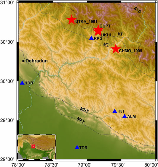
FIGURE 1. Map showing location of earthquakes (red asterisk) and distribution of recording stations (Green triangles).

Therefore, we propose to simulate the ground motions from these two earthquakes by adopting a well-known stochastic point source modeling technique. The technique assumes the spectral amplitude of the ground motion with the engineering notion that high-frequency motions are basically random vibrations (Hanks, 1979; Mc Guire and Hanks, 1980; Hanks and Mc Guire, 1981; Boore, 2003). The source of these random vibrations (earthquake) is assumed as a circular point source (Brune’s model) and the amplitude spectra follows ω⁻² fall with frequency. It is a simple technique that has been as successful as more sophisticated methods in predicting ground motion amplitudes over a broad range of magnitudes and distances. In spite of its popularity, this technique has certain limitations which cannot be neglected, especially when the distance between the source to site does not offer the agreement for point source assumption, that is, if source dimension <= epicenter distance. The technique does not consider the rupture geometry and directivity effects which cannot be ignored in case of large-magnitude earthquakes. Therefore, the finite fault approach is a preferable tool, especially for near-field simulations that can account for both fault and the directivity effects (Beresnev and Atkinson, 1997). Nevertheless, stochastic modeling has considerable advantage for being simple. The technique requires little or no information on the slip distribution on fault. Therefore, it becomes a good modeling tool for past earthquakes as well as for future events with unknown slip distributions.

Thus, our study expresses that the simple assumption of ω⁻² circular point source (Brune’s model) is good enough to synthesize seismograms from moderate-size earthquakes. In this article, we have made an attempt to reproduce the time histories by using the already-reported parameters required for simulation such as medium properties in terms of quality factor published in various literature works. An average value of the attenuation property of the medium, that is, quality factor (Q_s = 130.4*(f^0.998) (Knopoff, 1964) reported by many studies (see Gupta and Kumar, 2002; Parvez et al., 2003, Joshi, 2006a; 2006b; Chopra et al., 2012; Sharma et al., 2014; Harinarayan and Kumar, 2018) for Western Himalayas is used and found reliable to reproduce the strong ground motion (herein after SGM) in good agreement with the observed data. We emphasize that averaging the parameter values from many studies that focused on the same region will reduce the associated error of the parameters and deliver the optimum values useful for the modeling. We estimated the suitable stress drop values for both the earthquakes by generating a number of time histories and comparing the RMS error for each value of stress drop between the observed and predicted PGA values. The stress drop estimated for Guptakashi (mb = 5.6) and Ukhimath (mb5.1) are 73 and 105 bars, respectively. The values are very well in comparison with the values obtained by Joshi, 2006a, 2006b; Chopra et al., 2012; Sharma et al., 2014.

This study also emphasizes the contribution from the local site effect. The local site effect is proposed to obtain empirically which generally shows very large variations as compared to the source and medium properties. Therefore, in this study, the modeled acceleration spectra is structured by using source and medium information at first, and then it is corrected by the local site effects beneath each recording station, which is estimated empirically using the H/V method (Nakamura, 1989; 2008).

The site-corrected spectra (herein after synthetic acceleration spectra) are then compared with the Fourier amplitude spectra (herein after FAS) of the observed accelerograms obtained from the recorded waveform data. The comparison is done for frequency ranges between 0.1 and 10 Hz.

The synthetic acceleration spectra are then inverted to obtain the stochastic time series (synthetic accelerograms) and compared with observed accelerograms for amplitude (peak ground accelerations, PGA). There is a good agreement between the observed and predicted peak ground accelerations. This indicates that the considered parameters such as stress drop and attenuation properties are appropriate for strong ground motion modeling in this region.

The response spectra with 5% damping at different structural periods is also obtained from the synthetic and recorded accelerograms. The modeled pseudo spectral accelerations (PSA), velocity (PSV), and displacement (PSD) obtained are compared with the observed ones for both the earthquakes at each station.

The observed and estimated PGA values are also compared with existing GMPEs for shallow crustal seismicity (see results and discussion section). The above mentioned work on the simulation of strong ground motions is encouraging and can be adopted to predict the ground motion parameters like PGA at different distances for a hypothesized moderate to large magnitude earthquake for example, say M = 7.0 or more. However, it is emphasized that the site effect must be obtained empirically so that the observed acceleration spectra are inclusive of the local site effect. The details of data processing, methodology, and results are discussed in the following sections.

The confidence level and mismatch between the simulations and recorded data is expressed by associating the predictions with standard deviations, which are calculated from distribution of residuals (log₁₀Y^obs—log₁₀Y^pred), that is, common log difference between the observed and simulated data.

It is highlighted that this study is carried out to propose the idea to experiment with the existing parameters obtained from the larger dataset and check the reproducibility of ground motions and the reliability of model parameters even for small datasets. The estimated results obtained by the proposed approach assure the purposefulness of quick estimation of PGA values and preserve the reliability of ground motion parameters.

Data Processing

Two earthquakes of magnitude mb = 5.6 and mb = 5.1 occurred in the Uttarakhand region on 06/02/2017 and 06/12/2017 (Guptakashi and Ukhimath earthquakes, respectively). These earthquakes were well recorded at five stations, namely, Almorah (ALM), Haridwar (HDR), Rudraprayag (RPG), Thakurdwar (TDR), and Tarikhet (TKT) which are equipped with strong-motion broadband velocity seismographs (for details, refer Chadha et al., 2016). The recorded waveforms are converted into accelerations after applying instrument correction. The mean and the trend were also removed. Then, a zero-phase shift, Butterworth filter in the frequency band between 0.1 and 10 Hz is applied. The station location along with the epicenters is shown in Figure 1. The hypocenter parameters of the earthquakes are mentioned in Table 1.

TABLE 1

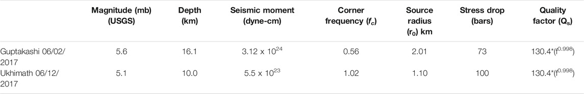
TABLE 1. Description of the source and medium parameters used for simulation.

Theory and Methodology

The stochastic method adopted in this article is construed from Boore, 2003; 2009. The basis of this technique can be cited through the works of Hanks, 1979; Mc Guire and Hanks, 1980; Hanks and Mc Guire, 1981. The technique assumes that the seismic signal recorded from the far field can be considered as band-limited, finite-duration, white Gaussian noise, and that the source spectra are described by a single corner frequency model whose corner frequency is proportional to the earthquake size. According to Brune (1970, 1971), the source scaling is expressed as f_c ∼ ω⁻².

The three main elements which constitute the seismic waveform are source (earthquake), path (the medium through which the seismic waves propagate), and the site at which the receivers are deployed and the waveform gets recorded.

These ground motions recorded by the seismograph (ground accelerations) can be expressed as a convolution of the above mentioned source, path, and site effects, which is mathematically represented by the following functional form (Eq. 1) (Boore and Atkinson, 1987):

$A\left(f\right)=C\cdot M_o\cdot S\left(f\right)\cdot D\left(f\right)\cdot \mathit{SE}\left(f\right),(1)$

where A(f) is the acceleration spectra, C is a constant, M_o is the seismic moment, SE(f) is the site effect, S(f) represents the source function, and D(f) represents the frequency dependent attenuation function, that is, medium effect.

The source function in the frequency domain is represented in Eq. 2:

$S\left(f\right)=\frac{{\left(2\cdot \mathrm{pi}\cdot f\right)}^2}{1+{\left(f/f_c\right)}^2},(2)$

where f_c is the corner frequency which is expressed as $f_c=2.34\beta /2\pi r_o$, $\beta$ is the shear wave velocity in the crust (here it is 3.5 km/s), and r₀ is the source radius which is obtained through the stress drop and seismic moment as mentioned in Eq. 3:

$\Delta \sigma =0.4397\cdot M_0/r_0^3,(3)$

$C=\frac{R_{\mathrm{\theta }\mathrm{\varphi }}\cdot \mathrm{FS}\cdot \mathrm{PR}}{4\mathrm{\pi }\mathrm{\rho }{\mathrm{\beta }}^3}.(4)$

The constant C represented in Eq. 4 is considered as the important factor for any site for a given earthquake. It is preferred for a double couple model embedded in an elastic medium, while considering only the S waves (Boore, 1983). It accounts for the combined effects of the radiation pattern (R_θΦ =0.55), free surface effect FS (here it is 2), partition of energy into two horizontal components PR (here it is 1/√2), and density ρ (here 2.67 g/cm³) and the shear wave velocity β (here 3.5 km/s), for the upper crust, respectively.

The decay of acceleration spectra due to elastic and anelastic attenuation (geometric and scattering effects) is represented by the Eq. 5:

$D\left(f\right)=\frac{e^{\left(-\mathrm{\pi }\mathrm{f}\mathrm{R}\right)/\left(\mathrm{Q}\mathrm{\beta }\right)}}{R}\cdot P\left(\mathrm{f},{\mathrm{f}}_{\max }\right),(5)$

where R is the hypocentral distance and P(f_min, f_max) represents the high-cut filter which can be interpreted as attenuation near the recording site (Hanks, 1982), with f_max = 10 Hz is used here (Joshi, 2006a; 2006b, V. Sri Ram et al., 2005).

The quality factor Q_s (Knopoff, 1964) in exponential term accounts for the anelastic attenuation and scattering nature of the medium.

Selection of Parameters

Source Parameters

The source parameters like seismic moment and stress drop of the Guptakashi and Ukhimath earthquakes are mentioned in Table 1. The parameter like seismic moment is obtained by using the definition proposed by Johnston (Johnston., 1996), expressed in Eq. 6. The seismic moment obtained is as follows:

$\mathrm{lo}{\mathrm{g}}_{10}{M}_o=18.75+0.496mb+0.0946m{b}^2.(6)$

This relation is also used to obtain the moment magnitude M_w by using the definition proposed by Hanks and Kanamori 1979, as expressed in Eq. 7.

$M_w=\frac{2}{3}\mathrm{lo}{\mathrm{g}}_{10}{M}_o-\mathrm{10.7.}(7)$

It appears that M_w for both Guptakashi and Ukhimath earthquakes are equal to mb; thus, we decided to retain the magnitude scale in mb for the sake of clarity.

The source parameter in the term stress drop value is estimated via the number of iterations. The values are assumed to be normally distributed ranging between 35 and 200 bars. Then the stress drop values are randomly extracted from the distribution. The time series is generated for each value to stress drop, along with all other path and site effect parameters (see sections below) and compared with the observed PGA values. The stress drop with the minimum RMS error is chosen and considered for the final simulation and modeling of the response spectra (Figure 2). The stress drop values obtained are 73 and 105 bars for Guptakashi (mb = 5.6) and Ukhimath (mb5.1) earthquakes, respectively.

FIGURE 2

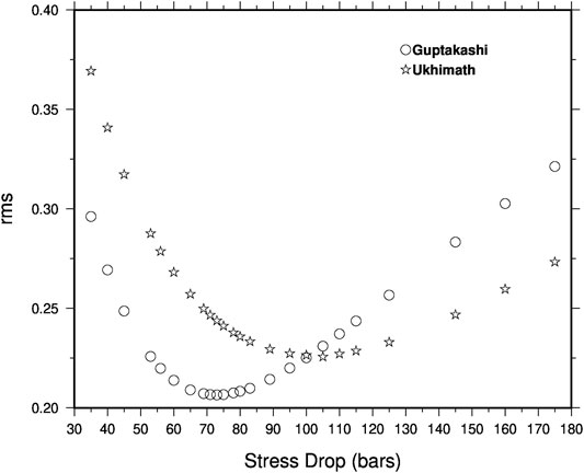
FIGURE 2. RMS errors with respect to the stress drop values used for simulations of time histories for both Guptakashi and Ukhimath earthquakes.

Moreover, the work of Joshi, 2006a, 2006b; Chopra et al., 2012; Sharma et al., 2014; Kumar et al., 2014 suggest the similar values for the stress drop for the western Himalayan region.

These values are further used to calculate the corner frequency fc and the source radius r₀ of both the Guptakashi and Ukhimath earthquakes for the analysis (please refer to Table 1 for the values). It should be noted that the estimation of stress drop is very critical and depends upon earthquake to earthquake. These values should be estimated for each source to minimize the random effects on the uncertainties associated with the source.

Path Effect Q and R

The decay of seismic waves with distance is classified by geometrical spreading and the aneslastic effect of the medium. Therefore, we consider the anelastic effect of the medium as an average value of the quality factor Q_s = 130.4*(f^0.998) obtained from different studies [see Parvez et al., 2003 (Q = 127f^0.96), Joshi, 2006a (Q = 112f^0.97), Sharma et al., 2014 (Q = 159f^1.16), Harinarayan and Kumar, 2018 (Q = 105f^0.94), and Gupta and Kumar, 2002 (149f^0.95)] to account for the attenuation effect due to the medium. The decay associated with geometrical spreading is accounted as the inverse of distance (1/R). The hypocentral distance R is derived from the depth and epicentral distance information from the catalog available at USGS (https://earthquake.usgs.gov).

It is to emphasize here that we prefer the average values because the averaging not only reduces the overall errors associated with the considered parameters but also furnish the combined contributions from the individual studies done to estimate the source and the medium property of the studied region.

Time Duration and Envelop

The choice of length of the envelop and the criteria for time duration of the vibration is based on the suggestions made by Boore, 2003; Saragoni and Hart (1974). The following equations are used to shape the envelop (see Eqs. 8–11) and to determine the time duration of a synthetic seismogram (see Eqs. 12, 13):

$\mathrm{wt}=\mathrm{a}{\left(t/t_{\eta }\right)}^b\cdot \exp \left(-c\cdot \left(t/t_{\eta }\right)\right),(8)$

where a, b, and c values are determined such that the function wt should have a peak amplitude of unity. The equations for a, b, and c are as follows:

$b=-\left(\mathit{ϵ}\cdot \ln \left(\eta \right)\right)/\left(1+\mathrm{ϵ}\cdot \ln \left(\mathit{ϵ}\right)-1\right),(9)$

$c=b/\mathit{ϵ},(10)$

$a={\left(\exp \left(1\right)/\mathit{ϵ}\right)}^b.(11)$

The values used to designed the window are $\eta =0.05$ and $\mathrm{ϵ}=0.2$ (see Saragoni and Hart, 1974; Boore, 2003).

The duration of the window is defined by the equations below:

$t_{\eta }=\mathrm{f}{\mathrm{T}}_{\mathrm{gm}}\cdot T_{\mathrm{gm}},(12)$

$T_{\mathrm{gm}}=1/f_c+0.5\cdot R,(13)$

where R is the hypocentral distance and $f{T}_{\mathrm{gm}}=2.0$.

Local Site Effect

The local site effect varies from site to site, and these variations are large as compared to the source and medium properties. Thus, we prefer to obtain the site factor empirically by adopting the method popularly known as the H/V ratio method (see Nakamura, 1989; 2008). The technique was further extended by Lermo and Garcia (Lermo and Chávez-García, 1993). This is based on the shear wave spectral ratio of the horizontal components to the vertical component. This method nullifies the effect from the source and propagating medium, therefore endorsing the effect of local geological site conditions at a shallow level.

Many studies like those by Oubaiche et al., 2016, Nakamura (1989, 2000, 2009), Konno and Ohmachi (1998), and Bonnefoy–Claudet et al. (2008) have found a strong correlation between H/V and SH transfer function. The H/V ratio is used as a transfer function which provides the level of site amplification, but in a broader manner. Therefore, an average value within the frequency range from 0.1 to 10 Hz is used as a site amplification factor (Field and Jacob, 1993) (see Figure 3). Nevertheless, it should be kept in mind that this does not provide the quantitative estimation of site amplification but it gives the comprehensive idea of the site effect when compared with Vs30 values. In this case, site amplification is considered as a random variable and obtained empirically. It is to be noted that the scarce dataset and for the sake of simplicity, we considered it as a consolidated factor of site amplification and multiplied as a scalar value with the modeled acceleration spectra to get the site-corrected spectra (synthetic acceleration spectra) at each station.

FIGURE 3

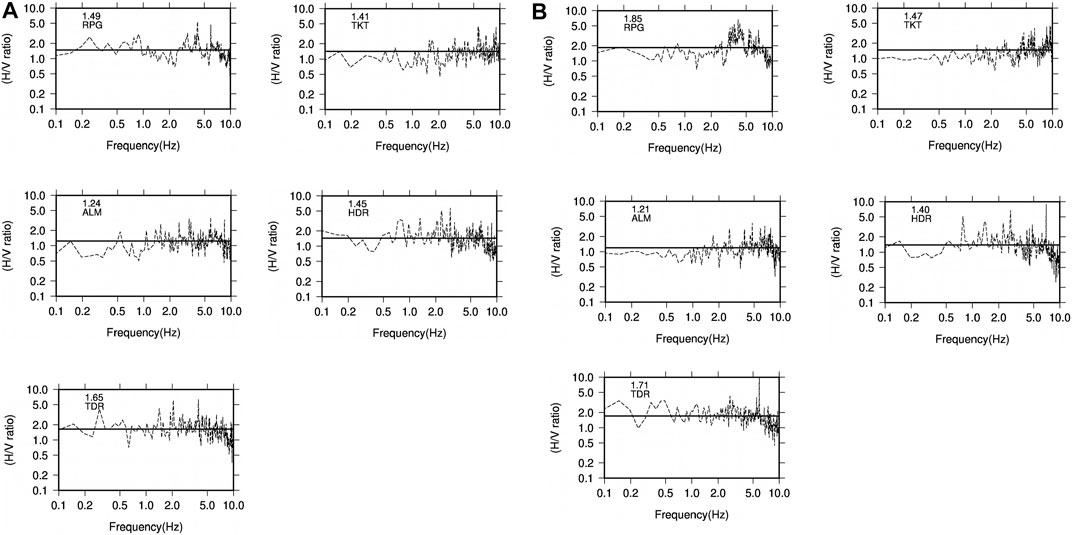
FIGURE 3. Plots of H/V ratio at each station for Guptakashi earthquake (3a) and Ukhimath earthquake (3b). The solid line represents the mean value of H/V ratio for all the considered frequency ranges (0.1–10 Hz). The mean values used as the site amplification factor are also mentioned in the plots.

The synthetic acceleration spectra are converted to acceleration time histories through the inverse Fourier transform. It is a very crucial step where the number of Fourier points should be kept beyond the time domain signal length. This is achieved by padding zero to get the nearest value in terms of power of 2.

Hence, the synthetic accelerations time histories are compared with the observed time series in terms of PGA. The details are discussed in the next section.

Results and Discussion

The stochastic simulation of two earthquakes, Guptakashi and Ukhimath with magnitudes mb = 5.6 and mb = 5.1, which occurred at shallow depths of 16.1 and 10 km, respectively, has been attempted. These events are located between the epicenters of 1991 Uttarkashi (M_w 6.8) and 1999 Chamoli (M_w 6.5) earthquakes. This zone is capable of yielding a large magnitude earthquake in near future (Khattri and Tyagi, 1983; Yeats and Thakur, 1998). All the information (location, magnitude, etc.) of the earthquakes used for simulation purposes is obtained from public domain agencies [United States Geological Survey (NEIC and USGS)]. Both earthquakes are recorded at five stations [Almorah (ALM), Haridwar (HDR), Rudraprayag (RPG), Thakurdwar (TDR), and Tarikhet (TKT)] located within the hypocentral range from 14 to 170 km (Figure 1). The maximum PGA observed at the nearest station RPG is 165.52 and 167.255 cm/s² station for Guptakashi and Ukhimath earthquakes, respectively. This brings Rudrapyag district (RPG) under moderate to severe intensity zone category.

The S waves from the horizontal components are considered for the analysis. The modeled spectra are obtained by using the source and medium information as discussed in the methodology section above.

The synthetic acceleration spectra are then obtained by correcting the modeled spectra by the site amplification factor obtained after H/V ratio (Nakamura, 2008). The H/V ratio is obtained between 0.1 and 10 Hz (see Figures 3A,B) at each station and for both the earthquakes separately (see Table 1, 2). The mean site amplification factor ranges between 1.2–1.8. This might be due to the fact that most of the sites are either rock sites or hard soil, which is not causing very high amplifications (Anbazhagan et al., 2019). The mean value of H/V ratio is calculated for this frequency range and multiplied with the modeled spectra to obtain the final corrected modeled spectra, that is, synthetic acceleration spectra. It is worth to mention here that through this practice, the station effects considered here are not based on the average V_S30 values but include in a more general way to consider the site effects concurring to a systematic site amplification or attenuation. It is mentioned in the section above that with the constrained dataset, we considered the transfer function as a scaling factor to correct the modeled acceleration spectra for site effects. The FAS of recorded S waves (NS and EW) are then compared with the synthetic acceleration spectra (see Figures 4A,B).

TABLE 2

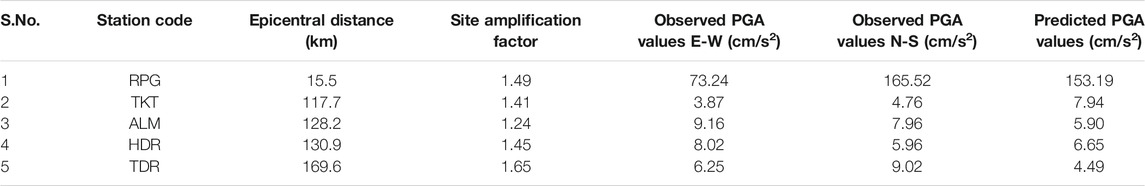
TABLE 2. Table showing station codes, site amplification factor, observed and predicted PGA values, and standard errors among FAS for Guptakashi earthquake, M_b = 5.6, 06/02/2017.

FIGURE 4

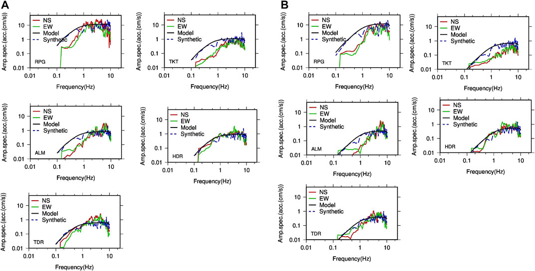
FIGURE 4. Comparison of the observed and synthetic Fourier amplitude spectra (FAS) for Guptakashi earthquake (4A) and Ukhimath earthquake (4B). The comparison shows good match between modeled and observed ones..

It is interesting to note that even though with the general values of source and medium properties, the synthetic acceleration spectra provide reasonable estimates of the general shape and amplitudes of the spectra for most of the stations. The mismatch is observed at lower frequencies specially for the nearest stations like RPG, TKT, and ALM, but with an increase in the distance, the modeled and observed spectra match well even at low frequencies (HDR and TDR). It can be due to the adoption of the fixed rupture velocity used for the simulation of strong ground motions. In fact, the point source approximation is not always realized at all the epicentral distances.

Nevertheless, the synthetic accelerograms obtained by the inverse of FAS (see the methodology section) shows good agreement with the observed accelerograms, specifically in term of amplitudes. The recorded and simulated seismograms for both Guptakashi and Ukhimath earthquakes at each station are illustrated in Figures 5A,B. The predicted and observed PGA values for both Guptakashi and Ukhimath earthquakes can be seen Tables 2, 3. The predicted values agree with the NS components because they are aligned with the radial component.

FIGURE 5

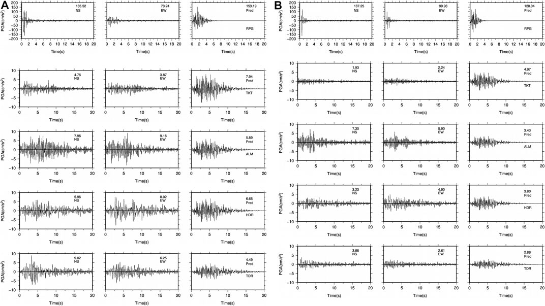
FIGURE 5. Comparison of recorded horizontal (NS and EW) components of accelerograms and the synthetic accelerograms for both Guptakashi (5A) and Ukhimath earthquakes (5B). The PGA values are mentioned along with the horizontal component and station codes.

TABLE 3

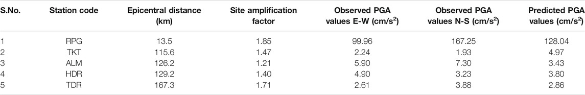
TABLE 3. Table showing station codes, site amplification factor, observed and predicted PGA values, and standard errors among FAS for Ukhimath Earthquake, M_b = 5.1, 06/12/2017.

We believe that the ground motion estimation should also serve the purpose of civil engineers, as they are more interested in spectral accelerations at different structural periods. Therefore, keeping it in mind, we also calculated the pseudo spectral accelerations (PSA), velocity (PSV), and displacement (PSD) with standard 5% damping factors at different structural periods ranging between 0.1 and 10 s. The spectral ordinates are calculated at each station and for both the earthquakes (Figures 6A,B). These spectral acceleration, velocities, and displacement obtained from the observed data are compared with the synthetic ones.

FIGURE 6

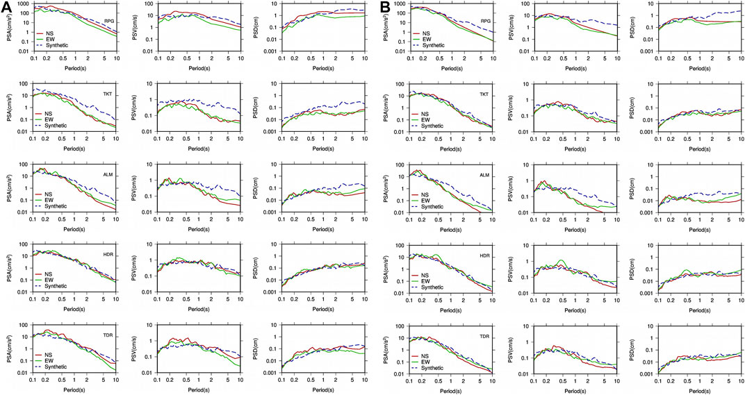
FIGURE 6. Pseudo spectral accelerations, velocities, and displacements estimated from the observed data and its comparison with the synthetic one.

There are deviations observed specially at lower frequencies, which result in under- and over-prediction of the observed response spectra. Even though the general shape of the response spectra is maintained for synthetic data, these deviations are predominant before 0.5 s, especially at RPG, TKT, and ALM stations. The predictions at lower period are overestimated. The distant stations HDR and TDR have an overall good match. This mismatch reminds the fact that there are some random factors which might not be fully captured during the evaluation of source (e.g., stress drop), medium (Q_s, quality factor), and site properties. The synthetic models do have some limitations in defining the complex source, medium, and site properties perfectly. Moreover, the point source approximations cannot be achieved at all the source to receiver distances.

Further, we have used the mean values which vary from region to region, especially the Q_s value, which also varies with epicentral distances, but we have considered the common and averaged attenuation value for all the stations. The epistemic uncertainties associated with model parameters specifically with the Qs and site effect will definitely affect the results. We tried to encounter random effects associated with earthquake uncertainties. We estimated stress drop values for the individual earthquakes by iteratively generating a number of time histories using different values of stress drop. The values which provide minimum RMS errors are considered for simulations (see Figure 2). Overall, we found good agreement between observed and predicted data in terms of both amplitudes and the response spectra.

Residual Analysis

We estimated the residuals which is common logarithmic (log₁₀) difference between the observed (NS and EW components) and the predicted PGA values for both the earthquakes at each station (see Figure 7). It is observed that the total scattering of residuals lies between +0.33 and −0.41 and total standard deviation estimated is 0.22. The computed residuals for each station demonstrates how well the simulations replicate the real data. The work by Bommer et al., 2004 and Strasser et al., 2008 with 40 years of data also summaries the values of standard deviations which tend to lie between 0.15 and 0.35 in log₁₀ units for most of the ground motion prediction models. This further clarifies that our proposed idea is very well justified.

FIGURE 7

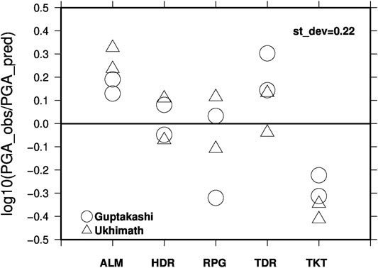
FIGURE 7. Comparison of the observed and predicted PGA values with GMPEs are shown here. The solid line indicates the mean values and +/− 1sigma is represented by the dashed lines. Asterisks represent the predicted values and the observed PGA values are represented by circles.

Comparison With Existing GMPEs

The results motivated us to compare our predicted and observed PGA values with some of the popular GMPEs developed for Western Himalayas and similar shallow crustal seismic environment. It is very interesting to note that our predicted and observed values are very well explained by some of the robust GMPEs, while some of the equations under/over predict our PGA values either at small distances or at large distances. The GMPEs, for example, developed by Emolo et al., 2015 for the south Korean Peninsula, and the GMPEs developed by Bommer et al., 2003 for European scenarios appeared to explain the observed and predicted PGA values within +/−1 sigma at small distances as compared to large distances (see Figure 8). While the GMPEs developed by Iyenger and Gupta, 2004; Joshi et al., 2012 could not explain the data very well at small distances, they over predicted the PGA values for Guptakashi earthquake. This must be due to the regional dependencies which must be taken into account while developing or selecting the GMPEs to perform seismic hazards. Overall, the GMPES could not convincingly explain the observed values for small to large distance ranges even though the magnitude is kept same. Therefore, it is to emphasize the fact that there is always a need to update the ground motion prediction models with the addition of more data in terms of broad magnitude and distance ranges.

FIGURE 8

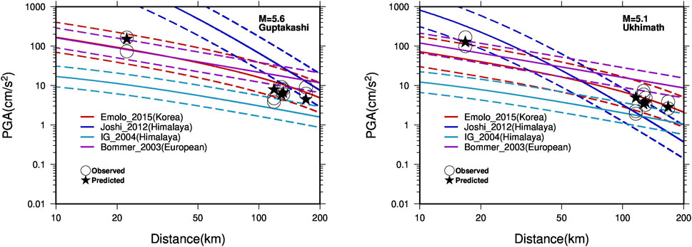
FIGURE 8. Distribution of residuals for the PGA values at each station for both Guptakashi and Ukhimath earthquakes.

The present study emphasizes the prospects to reproduce the results for different earthquakes by using the model parameters, which are already obtained by other studies through inversion of large datasets in the same region. Moreover, this work also proposed the idea to experiment with the parameters obtained from the largest dataset and check the reproducibility of ground motions with these parameters even for small datasets.

This idea will not only help in gaining clarity over existing studies but also help in identifying the uncaptured properties of the source, medium, and site to minimize the associated errors by refining the model parameters. For example, the aleatory and epistemic uncertainties associated with model parameters should always be considered while modeling the ground motion, especially when there is a larger dataset.

Conclusion

1) The stochastic modeling technique is adopted to simulate strong ground motions. The simulation is done for two earthquakes that occurred in Uttarkashi with magnitude M > 5 on 06/02/2017 and 06/12/2017 [Guptakashi (mb = 5.6) and Ukhimath (mb = 5.1), respectively].

2) The synthetic spectra shows good agreement with the observed Fourier amplitude spectra (FAS) obtained from the recorded waveform data. The stochastic time series is also compared with the observed waveforms in terms of amplitude (PGA). The response spectra obtained from the simulated waveform and from the observed ones were found to be a good match, when compared.

3) The overall good match between the observed and predicted ground motion parameters prove that the simple assumption of circular crack model (ω⁻², point source) and parameters derived from public agencies are sufficient enough for the model, and the ground motions are generated from earthquakes.

  1) The mismatch observed at lower frequencies, especially at near field stations, can be due to the adoption of fixed rupture velocity used for the simulation of strong ground motions. Moreover, the simple/point source model does have some limitation in defining the complex source, medium, and site properties perfectly.

  2) The random or between-event uncertainties should be considered while modeling the ground motion, when associated with the different sources even in the same region. The epstemic uncertainties associated with the medium might decrease with the addition of information unlike aleatory uncertainties.

  3) These preliminary results obtained not only validate the technique but are also encouraging to extend the technique further and to simulate strong ground motions for a hypothetical large magnitude earthquake for M = 7.0 and above in the Himalayan region.

  4) Such techniques are very useful in anticipating the potentially damaged zone for the future earthquake, and hence mitigating the seismic hazard.

  5) The comparison of our predictions and observed PGA data with existing GMPEs shows that our predictions are very well explained by many robust GMPEs developed for similar shallow crustal seismic environment in Asia and Europe. Moreover, it is also observed that there are certain discrepancies in the predicted PGA values and can be ascribed to the fact that the ground motion parameters are region specific; hence, prediction models are needed to be developed and updated with time. Therefore, in a nutshell, it can be concluded that the proposed work and results obtained in this study are very optimistic and contribute toward the understanding of strong ground motions in the Himalayan region.

Data and Resources

The seismograms used in this study were recorded by stations from the Indo-Gangetic Plains network (CIGN), maintained by the Council of Scientific and Industrial Research-National Geophysical Research Institute (NGRI). The earthquake information used for simulation purpose is obtained from the catalog available at the United States Geological Survey (NEIC and USGS), https://earthquake.usgs.gov/.

Data Availability Statement

The raw data supporting the conclusions of this article will be made available by the authors, without undue reservation.

Author Contributions

NS designed the problem, carried out the analysis, and drafted the manuscript. DS suggested necessary modifications in the manuscript. GS and DS retrieved the data from the stations and provided instrument information.

Conflict of Interest

The authors declare that the research was conducted in the absence of any commercial or financial relationships that could be construed as a potential conflict of interest.

Publisher’s Note

All claims expressed in this article are solely those of the authors and do not necessarily represent those of their affiliated organizations, or those of the publisher, the editors, and the reviewers. Any product that may be evaluated in this article, or claim that may be made by its manufacturer, is not guaranteed or endorsed by the publisher.

Acknowledgments

The authors acknowledge the support and grant received from the projects MLP—6401-28 (DSN) of National Geophysical Research Institute funded by Council of Scientific and Industrial Research, Government of India. The authors are also thankful to the Director, CSIR—NGRI, Hyderabad, for his kind support and permission to publish the research work. All the figures are prepared using the Generic Mapping tool (Wessel and Smith, 1991). The simulation is done using MATLAB Software. The authors are extremely thankful to the editor and the reviewers for their constructive comments which have definitely improve the study and the manuscript.

References

Anbazhagan, P., Srilakshmi, K. N., Bajaj, K., Moustafa, S. S. R., and Al-Arifi, N. S. N. (2019). Determination of Seismic Site Classification of Seismic Recording Stations in the Himalayan Region Using HVSR Method. Soil Dyn. Earthquake Eng. 116, 304–316. doi:10.1016/j.soildyn.2018.10.023

CrossRef Full Text | Google Scholar

Beresnev, I. A., and Atldnson, G. M. (1997). Modeling Finite-Fault Radiation from the 09 N Spectrum. Bull. Seism. Soc. Am. 87, 67–84.

Google Scholar

Bilham, R., Gaur, V. K., and Molnar, P. (2001). Himalayan Seismic Hazard. Science 293 (5534), 1442–1444. doi:10.1126/science.1062584

PubMed Abstract | CrossRef Full Text | Google Scholar

Bommer, J. J., Abrahamson, N. A., Strasser, F. O., Pecker, A., Bard, P.-Y., Bungum, H., et al. (2004). The challenge of Defining Upper Bounds on Earthquake Ground Motions. Seismological Res. Lett. 75 (1), 82–95. doi:10.1785/gssrl.75.1.82

CrossRef Full Text | Google Scholar

Bommer, J. J., Douglas, J., and Strasser, F. O. (2003). Style-of-Faulting in Ground-Motion Prediction Equations. Bull. Earthquake Eng. 1, 171–203. doi:10.1023/A:1026323123154

CrossRef Full Text | Google Scholar

Bonnefoy-Claudet, S., Köhler, A., Cornou, C., Wathelet, M., and Bard, P.-Y. (2008). Effects of Love Waves on Microtremor H/V Ratio. Bull. Seismological Soc. America 98 (1), 288–300. doi:10.1785/0120070063

CrossRef Full Text | Google Scholar

Boore, D. M., and Atkinson, G. M. (1987). Stochastic Prediction of Ground Motion and Spectral Response Parameters at Hard-Rock Sites in Eastern North America. Bull. Seismological Soc. America 77 (2), 440–467.

Google Scholar

Boore, D. M. (2009). Comparing Stochastic point-source and Finite-Source Ground-Motion Simulations: SMSIM and EXSIM. Bull. Seismological Soc. America 99 (6), 3202–3216. doi:10.1785/0120090056

CrossRef Full Text | Google Scholar

Boore, D. M. (2003). Simulation of Ground Motion Using the Stochastic Method. Pure Appl. Geophys. 160, 635–676. doi:10.1007/PL00012553

CrossRef Full Text | Google Scholar

Boore, D. M. (1983). Stochastic Simulation of High-Frequency Ground Motions Based on Seismological Models of the Radiated Spectra. Bull. Seismol. Soc. Am. 73, 1865–1894.

Google Scholar

Chadha, R. K., Srinagesh, D., Srinivas, D., Suresh, G., Sateesh, A., Singh, S. K., et al. (2016). CIGN, A Strong‐Motion Seismic Network in Central Indo‐Gangetic Plains, Foothills of Himalayas: First Results. Seismological Res. Lett. 87 (1), 37–46. doi:10.1785/0220150106

CrossRef Full Text | Google Scholar

Chopra, S., Kumar, V., Suthar, A., and Kumar, P. (2012). Modeling of strong Ground Motions for 1991 Uttarkashi, 1999 Chamoli Earthquakes, and a Hypothetical Great Earthquake in Garhwal-Kumaun Himalaya. Nat. Hazards 64, 1141–1159. doi:10.1007/s11069-012-0289-z

CrossRef Full Text | Google Scholar

Emolo, A., Sharma, N., Festa, G., Zollo, A., Convertito, V., Park, J. H., et al. (2015). Ground‐Motion Prediction Equations for South Korea Peninsula. Bull. Seismological Soc. America 105 (5), 2625–2640. doi:10.1785/0120140296

CrossRef Full Text | Google Scholar

Field, E., and Jacob, K. (1993). The Theoretical Response of Sedimentary Layers to Ambient Seismic Noise. Geophys. Res. Lett. 20, 2925–2928. doi:10.1029/93gl03054

CrossRef Full Text | Google Scholar

Goda, K., Kiyota, T., Pokhrel, R. M., Chiaro, G., Katagiri, T., Sharma, K., et al. (2015). The 2015 Gorkha Nepal Earthquake: Insights from Earthquake Damage Survey. Front. Built Environ. 1, 8. doi:10.3389/fbuil.2015.00008

CrossRef Full Text | Google Scholar

Gupta, S. C., and Kumar, A. (2002). Seismic Wave Attenuation Characteristics of Three Indian Regions: A Comparative Study. Curr. Sci. 82, 407–413.

Google Scholar

H, H., and Kumar, A. (2018). Estimation of Source and Site Characteristics in the North-West Himalaya and its Adjoining Area Using Generalized Inversion Method. Ann. Geophys. 62 (5), SE559. doi:10.4401/ag-7922

CrossRef Full Text | Google Scholar

Hanks, T. C. (1979). Bvalues and ω−γseismic Source Models: Implications for Tectonic Stress Variations along Active Crustal Fault Zones and the Estimation of High-Frequency strong Ground Motion. J. Geophys. Res. 84, 2235–2242. doi:10.1029/jb084ib05p02235

CrossRef Full Text | Google Scholar

Hanks, T. C. (1982). f max. Bull. Seismological Soc. America 72, 1867–1879. doi:10.1785/bssa07206a1867

PubMed Abstract | CrossRef Full Text | Google Scholar

Hanks, T. C., and McGuire, R. K. (1981). The Character of High-Frequency Strong Ground Motion. Bull. Seismol. Soc. Am. 71, 2071–2095. doi:10.1785/bssa0710062071

CrossRef Full Text | Google Scholar

Iyenger, R. N., and Ghosh, S. (2004). Microzonation of Earthquake hazard in Greater Delhi Area. Curr. Sci. 87, 1193–1202.

Google Scholar

Johnston, A. C. (1996). Seismic Moment Assessment of Earthquakes in Stable continental Regions—I. Instrumental Seismicity. Geophys. J. Int. 124 (Issue 2), 381–414. doi:10.1111/j.1365-246x.1996.tb07028.x

CrossRef Full Text | Google Scholar

Joshi, A. (2006a). Analysis of strong Motion Data of the Uttarkashi Earthquake of 20th October 1991 and the Chamoli Earthquake of 28th March 1999 for Determining the Mid Crustal Q Value and Source Parameters. J. Earth Tech. 43, 11–29.

Google Scholar

Joshi, A. (2006b). Use of Acceleration Spectra for Determining the Frequency-dependent Attenuation Coefficient and Source Parameters. Bull. Seismological Soc. America 96, 2165–2180. doi:10.1785/0120050095

CrossRef Full Text | Google Scholar

Joshi, A., Kumar, A., Lomnitz, C., Castaños, H., and Akhtar, S. (2012). Applicability of Attenuation Relations for Regional Studies. Geofísica internacional 51 (4), 349–363. doi:10.22201/igeof.00167169p.2012.51.4.1231

CrossRef Full Text | Google Scholar

Khattri, K. M., and Tyagi, A. K. (1983). Seismicity Patterns in the Himalayan Plate Boundary and Identification of the Areas of High Seismic Potential. Tectonophysics 96, 281–297. doi:10.1016/0040-1951(83)90222-6

CrossRef Full Text | Google Scholar

Knopoff, L. (1964). Q. Rev. Geophys. 2 (4), 625–660. doi:10.1029/rg002i004p00625

CrossRef Full Text | Google Scholar

Konno, K., and Ohmachi, T. (1998). Ground-Motion Characteristics Estimated from Spectral Ratio between Horizontal and Vertical Components of Microtremor. Bull. Seismol. Soc. Am. 88, 228–241. doi:10.1785/bssa0880010228

CrossRef Full Text | Google Scholar

Kumar, S., and Sharma, N. (2019). The Seismicity of Central and North-East Himalayan Region. Contrib. Geophys. Geodesy 49 (3), 265–281. doi:10.2478/congeo-2019-0014

CrossRef Full Text | Google Scholar

Lermo, J., and Chávez-García, F. J. (1993). Site Effect Evaluation Using Spectral Ratios with Only One Station. Bull. Seismol. Soc. Am. 83 (5), 1574–1594. doi:10.1785/bssa0830051574

CrossRef Full Text | Google Scholar

McGuire, R. K., and Hanks, T. C. (1980). RMS Accelerations and Spectral Amplitudes of strong Ground Motion during the San Fernando, California Earthquake. Bull. Seismol. Soc. Am. 70, 1907–1919. doi:10.1785/bssa0700051907

CrossRef Full Text | Google Scholar

Nakamura, Y., (2008). “On H/V Spectrum,” in The 14th World Conference on Earthquake Engineering, Beijing, China, October 12-17, 2008.

Google Scholar

Nakamura, Y. (1989). A Method for Dynamic Characteristics Estimation of Subsurface Using Microtremor on the Ground Surface. Q. Rep. Railway Tech. Res. Inst. 30 (1), 25–30.

Google Scholar

Nakamura, Y. (2009). “Basic Structure of QTS (HVSR) and Examples of Applications,” in Increasing Seismic Safety by Combining Engineering Technologies and Seismological Data.NATO Science for Peace and Security, Series C: Environmental. Editors M. Mucciarelli, M. Herak, and J. Cassidy(Springer: Dordrecht).

Google Scholar

Nakamura, Y. (2000). “Clear Identification of Fundamental Idea of Nakamura’s Technique and its Applications,” in Proc. of the 12th World Conference on Earthquake Engineering, Auckland, New Zealand, 30 January 30–February 4, 2000.

Google Scholar

Oubaiche, E. H., Chatelain, J. L., Hellel, M., Wathelet, M., Machane, D., Bensalem, R., et al. (2016). The Relationship between Ambient Vibration H/V and SH Transfer Function: Some Experimental Results. Seismological Res. Lett. 87 (5), 1112–1119. doi:10.1785/0220160113

CrossRef Full Text | Google Scholar

Parvez, I. A., Vaccari, F., and Panza, G. F. (2003). A Deterministic Seismic hazard Map of India and Adjacent Areas. Geophys. J. Int. 155, 489–508. doi:10.1046/j.1365-246X.2003.02052.x

CrossRef Full Text | Google Scholar

Saragoni, G. R., and Hart, G. C. (1974). Simulation of Artificial Earthquakes. Earthq. Eng. Struct. Dyn. 2, 249–267.

Google Scholar

Sharma, J., Chopra, S., and Roy, K. S. (2014). Estimation of Source Parameters, Quality Factor (QS), and Site Characteristics Using Accelerograms: Uttarakhand Himalaya RegionQS), and Site Characteristics Using Accelerograms: Uttarakhand Himalaya Region. Bull. Seismological Soc. Americaulletin Seismological Soc. America 104 (1), 360–380. doi:10.1785/0120120304

CrossRef Full Text | Google Scholar

Strasser, F. O., Bommer, J. J., and Abrahamson, N. A. (2008). Truncation of the Distribution of Ground-Motion Residuals. J. Seismol 12 (1), 79–105. doi:10.1007/s10950-007-9073-z

CrossRef Full Text | Google Scholar

Yeats, R. S., and Thakur, V. C. (1998). Reassessment of Earthquake hazard Based on a Fault-bend Fold Model of the Himalayan Plate-Boundary Fault. Curr. Sci. 74, 230–233.

Google Scholar