 Christos Kourouklas
 Rodolfo Console2,3
 Eleftheria Papadimitriou
 Maura Murru
- 1Geophysics Department, School of Geology, Aristotle University of Thessaloniki, Thessaloniki, Greece
- 2Center of Integrated Geomorphology for the Mediterranean Area (CGIAM), Potenza, Italy
- 3Istituto Nazionale di Geofisica e Vulcanologia, Sezione Roma 1 (Seismology and Tectonophysics), Rome, Italy
The recurrence time, Tr, of strong earthquakes above a predefined magnitude threshold on specific faults or fault segments is an important parameter, that could be used as an input in the development of long-term fault-based Earthquake Rupture Forecasts (ERF). The amount of observational recurrence time data per segment is often limited, due to the long duration of the stress rebuilt and the shortage of earthquake catalogs. As a consequence, the application of robust statistical models is difficult to implement with a precise conclusion, concerning Tr and its variability. Physics-based earthquake simulators are a powerful tool to overcome these limitations, and could provide much longer earthquake records than the historical and instrumental earthquake catalogs. A physics-based simulator, which embodies known physical processes, is applied in the Southern Thessaly Fault Zone (Greece), aiming to provide insights about the recurrence behavior of earthquakes with Mw ≥ 6.0 in the six major fault segments in the study area. The build of the input fault model is made by compiling the geometrical and kinematic parameters of the fault network from the available seismotectonic studies. The simulation is implemented through the application of the algorithm multiple times, with a series of different input free parameters, in order to conclude in the simulated catalog which showed the best performance in respect to the observational data. The detailed examination of the 254 Mw ≥ 6.0 earthquakes reported in the simulated catalog reveals that both single and multiple segmented ruptures can be realized in the study area. Results of statistical analysis of the interevent times of the Mw ≥ 6.0 earthquakes per segment evidence quasi-periodic recurrence behavior and better performance of the Brownian Passage Time (BPT) renewal model in comparison to the Poissonian behavior.
Introduction
The study of the statistical behavior of strong earthquakes’ occurrence above a given magnitude threshold (e.g., M ≥ 6.0) on specific faults or faults segments is among the key components of the estimation of fault-based probabilistic seismic hazard assessment (PSHA). The main purpose of such studies is the determination of the mean recurrence time, Tr, between successive strong earthquakes and their variability, the latter of which can be used as an input in the application of either Poissonian or renewal (time-depended) long-term Earthquake Rupture Forecast (ERF) models in a specific time span (Field, 2015).
The accurate computation and evaluation of recurrence time statistical parameters is a prerequisite for both the better understating of its behavior and the precision of the forecast models. For this reason, the compilation of as many as possible records of strong earthquakes that occurred in individual fault segments is necessary. However, the amount of this observational data is limited, often between 3 and 10 observations (Ellsworth et al., 1999; Sykes and Menke, 2006), and the related catalogs (both historical and instrumental) are relatively short because of the earthquake cycle’s long duration in each given segment. In addition, paleoseismological event dating (e.g., Biasi et al., 2015) and slip-rate constrains (Ogata, 2002; Biasi and Thompson, 2018) could refine the parameters’ space when they are used in combination with alternative approaches, such as Bayesian inference methods (Fitzenz, 2018).
An alternative approach to support and improve the study of strong earthquakes’ recurrence behavior is the development and application of physics-based simulator algorithms. These algorithms model the earthquake occurrence via numerical simulations using various approximations about the known physical processes concerning the stress transfer and frictional properties, along with kinematic and dynamic constraints (Tullis, 2012a). Starting from the early works of Rundle 1988 and Robinson and Benites 1996, the concept of physics-based simulators became popular during the last decade, due to their ability to model and reproduce long earthquake occurrence records (ranging from thousands to millions of years). Thus, a large number of such algorithms have been proposed (e.g., Yikilmaz et al., 2010; Richards-Dinger and Dieterich, 2012; Ward, 2012; Schultz et al., 2017) and applied (e.g., Robinson et al., 2011 and Christophersen et al., 2017 in New Zealand; Shaw et al., 2018 in California).
In this context, Console et al. 2015 introduced a physics-based simulator algorithm based on the modeling of the rupture growth, considering the long-term slip rate constraints on fault segments, which were firstly applied in the Corinth Gulf fault system in Greece. The simulated seismicity yielded satisfactory results on the magnitude distribution of the simulated catalog, which is consistent with the observations, and, again, with the realistic and consistent space time behavior (e.g., clustering of strong earthquakes and aftershock generation). Over the years, the simulation algorithm had a revolutionary improvement, comprising new parameters for the identification of successive ruptures (Console et al., 2017) and the inclusion of the afterslip process, modeled by a decaying Omori-like power law (Console et al., 2018a). These improved versions were successfully applied to simulate the seismicity of Calabria (Console et al., 2017; Console et al., 2018b) and Central Apennines (Console et al., 2018a) in Italy. The latest version of the algorithm incorporates the effect of the Rate and State Constitutive law proposed by Dieterich 1994 in the physical processes, leading to a stochastic manner of nucleation with applications in Central Italy (Console et al., 2020) and Greece (Mangira et al., 2020).
The current version is applied in the Southern Thessaly Fault Zone (STFZ) in Central Greece, which consists of part of the extensional back arc Aegean region and characterized by WNW-ESE to E-W normal faulting (Papazachos et al., 1998; Goldsworthy et al., 2002; Figure 1B). During the 20th century, a series of six strong and destructive (Mw ≥ 6.0) earthquakes occurred in the study area (Figure 1A and Table 1). Papadimitriou and Karakostas 2003 showed that the stress transfer dominates the occurrence of strong earthquakes within the STFZ, which have been characterized as episodic since the active periods alternate with much longer quiescent periods. Although several strong earthquakes Mw ≥ 6.0 had occurred since the 16th century in the broader Thessaly area, a rather complete historical record reveals (Papazachos and Papazachou, 2002) that only two of them that occurred during the 18th century are related with the STFZ (white stars of Figure 1A and Table 1). As a consequence, the study area could be characterized as an active area with strong earthquake occurrence during the instrumental period, however, het lack of a satisfactory number of Mw ≥ 6.0 events per segment inhibits the identification of the corresponding mean recurrence time, Tr.
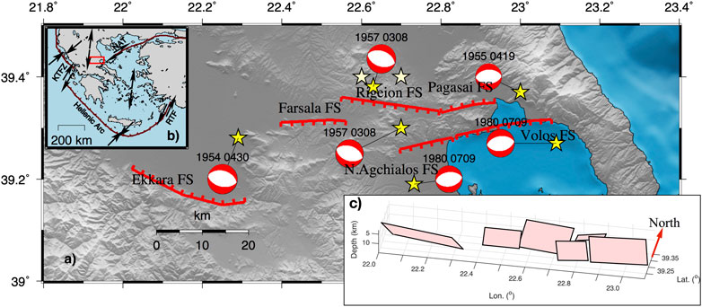
FIGURE 1. (A) Strong earthquake (Mw ≥ 6.0) occurrence in the Southern Thessaly Fault Zone. Yellow stars depict the Mw ≥ 6.0 events during the 20th century, whereas the white stars depict the historical ones during the 18th century. The six major segments of the Southern Thessaly Fault System are represented with the red solid lines and their names are also given. Focal mechanisms are plotted as lower-hemisphere equal-area projections. The occurrence date of each event is annotated on the top of focal spheres. (B) Main seismotectonic properties of the broader Aegean area along with the relative plate motions represented by the black arrows, either side of the active boundaries depicted by the thick red lines. The study area is denoted with a rectangular red box. (C) Schematic 3D representation of the six fault segments of the Southern Thessaly Fault Zone, modeled as rectangular planes for the current simulator application.
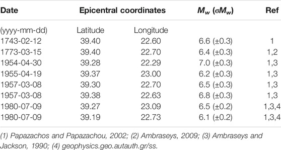
TABLE 1. Focal parameters of the Mw ≥ 6.0 strong earthquakes that occurred in the Southern Thessaly Fault Zone since 1700.
This fact provokes the detailed study of the long-term behavior of strong earthquakes via the application of the simulation algorithm with the ultimate goal of constructing built a large and representative strong earthquake record over a sufficient time span. This will form the basis for the statistical analysis of these earthquakes’ recurrence time behavior.
Seismotectonic Setting and Definition of the Fault Network of the Southern Thessaly Fault Zone
The active deformation in the broader Aegean region is dominated by the subduction of the oceanic lithosphere of the Eastern Mediterranean under the continental Aegean microplate, forming the Hellenic Arc and the extensional back arc region of the Aegean Sea (Papazachos and Comninakis, 1970; Papazachos and Comninakis, 1971; Figure 1B). The regional stress field of STFZ is characterized by a N-S extension, similar to the broader Aegean back arc area, with relatively moderate slip rates (about 4.6 ± 0.5 mm/yr) as derived from GPS measurements (Muller et al., 2013). The STFZ is composed of six sub-parallel major normal faults with an E-W to WNW-ESE strike (Figure 1A and Table 2), reaching maximum lengths of 15–25 km and typical dips for normal faulting equal to 45° (in agreement with Roberts, 1996; Roberts and Ganas, 2000; Goldsworthy and Jackson, 2000). The thickness of the seismogenic layer along the fault zone is equal to 12 km, with earthquake focal depths ranging between 3 and 15 km (Hatzfeld et al., 1999). The stress is mainly accumulated on and released through the six major fault segments, whose dimensions (Table 2) are large enough to be comparable with the seismogenic thickness of the upper crust and capable of rupturing in Mw ≥ 6.0 earthquakes (Goldsworthy and Jackson, 2000; Scholz, 2019).
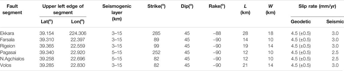
TABLE 2. Geometrical and kinematic parameters of the fault network model used in the simulation application of the Southern Thessaly Fault Zone.
The Ekkara fault segment with NW-SE strike (285°), NE dip, and length equal to 28 km is located at the westernmost part of the STFZ (Figure 1A), associated with the 1954 Mw = 7.0 earthquake (Papastamatiou and Mouyaris, 1986; Caputo and Pavlides, 1993). The 1954 event is the largest one known to have occurred in the study area and is also known as the Sofades earthquake due to the heavy damage caused by it in Sofades and neighboring villages (Ambraseys and Jackson, 1990; Papazachos and Papazachou, 2002; Papazachos et al., 2016).
Two distinctive groups of sub-parallel segments are its neighbors to the east. The fist group includes the Farsala, Rigeion, and Pagasai segments (Figure 1A). Farsala and Rigeion fault segments strike from E-W to ENE-WSW (89° and 99°, respectively), dip southwards, and extend in lengths of about 14 and 19 km, respectively (Caputo and Pavlides, 1993; Mountrakis et al., 1993). The third member of this group, the Pagasai fault segments strikes at 252°, dips north-northeastward, with a length equal to 12 km (Caputo and Pavlides, 1993; Galanakis et al., 1998). This group of fault segments is associated with a cluster of strong earthquakes from 1955 (just one year after the Ekkara main shock) up to 1957 that devastated the study area The 1955 Mw = 6.2 earthquake (Ambraseys and Jackson, 1990; Papazachos and Papazachou, 2002) occurred in the NE margin of the study area and is associated with the Pagasai fault segment. The activity continued by migrating westwards, filling in the gap between the 1954 and 1955 events, with the occurrence on the eighth of March 1957 doublet (with a time difference of 7 min; 12:14, Mw = 6.5 and 12:21, Mw = 6.8; Ambraseys and Jackson, 1990; Papazachos and Papazachou, 2002) causing heavy damage in the regions of Velestino, Farsala, and Volos. These two earthquakes, Mw = 6.5 and Mw = 6.8, are associated with the Farsala and Rigeion fault segments, respectively. It must be mentioned that, unless the Mw = 6.5 earthquake’s initial location is quite far from the Farsala segment (about 15–16 km), it is more likely to be associated with it rather than with the Rigeion segment because the latter cannot bear two strong events simultaneously. Convincing support for this argument is found in that the macroseismic effects, although difficult to be discriminated between the two main shocks, can be ascribed to both fault segments and the epicentral misallocation of that period due to the seismological network limitations.
The second group of the eastern part of the study area encompasses the Nea Agchialos (Galanakis et al., 1998) and Volos fault segments (Figure 1A), also identified by the seismic reflection survey of Perissoratis et al. 1991. These two segments strike at 82°, dip to the SE and with lengths equal to 21 and 12 km, respectively (Caputo, 1996; Galanakis et al., 1998). The Volos and Nea Agchialos segments are linked with a second doublet of strong earthquakes that occurred on the 9th of July 1980, with magnitudes equal to Mw = 6.5 (02:11) and Mw = 6.1 (02:35) (Papazachos et al., 1983; Ambraseys and Jackson, 1990; Drakos et al., 2001).
Papadimitriou and Karakostas 2003 studied the episodic occurrence of strong earthquake occurrence in a larger area, including the STFZ, and concluded that the stress transfer among adjacent fault segments is the dominant pattern. In the study area during the 18th century, two earthquakes of Mw = 6.6 and Mw = 6.4 occurred in 1743 and 1773, respectively (Table 1 and Figure 1A). These events are likely to be associated with the first group of easternmost faults segments (Farsala, Rigeion, Pagasai), but the lack of available historical information does not allow for a reliable linkage between them.
The available fault plane solutions show a rake angle equal to λ = −88° for the 1954 earthquake (McKenzie, 1972) associated with the Ekkara segment and λ = −90° for all the other fault segments (Papazachos et al., 2001). The thickness of the seismogenic layer along the fault zone is extended along 3 and 15 km (Hatzfeld et al., 1999), as already mentioned, except for the two smaller fault segments, namely the Pagasai and the Nea Agchialos, with lengths equal to 12 km, which are considered to be rooted in the middle of the seismogenic layer between the depths of 5 and 15 km.
The geodetic long-term slip rate equals 4.5 ± 0.5 mm/yr (Muller et al., 2013), is distributed homogenously along its segments, taking the larger part of the deformation. Taking into account that only the 60% of the total slip is released coseismically (Davis et al., 1997), the slip rate of each segment is assigned and given in Table 2. This estimate also agrees with Jenny et al. 2004 who concluded that the tectonic deformation in central Greece is not fully coupled but affected by aseismic creep. This conclusion is also supported by the recognition of anthropogenic-induced subsidence phenomena, as revealed by recent GNSS measurements (Argyrakis et al., 2020 and the references therein), which could be associated with the aseismic slip of the study area.
The slip rate values, corresponding to 60% percent of the total slip rate, are chosen to be equal to 3 mm/yr for the largest fault segments and 2.5 mm/yr for the smaller ones, rooted deeper in the seismogenic layer (Pagasai and Nea Agchialos; Table 2). These values are slightly higher and slightly lower, respectively, from the exact 60% (2.7 mm/yr), aiming to account in some way for the corresponding uncertainty of estimated values of the total slip.
All the aforementioned geometrical and kinematic parameters and data, as compiled from the previously mentioned studies, are taken into account in the definition of the fault network model for the study area, which is the main input of the simulation procedure, and are summarized in Table 2. The GreDass database (Caputo and Pavlides, 2013) and the 2020 updated version (v3.0) of NOA Faults (Ganas et al., 2013) are accessed in an attempt to compare the fault segments defined in this study and compare them with the ones defined in the two databases. This comparison (Supplementary Appendix A) revealed a good agreement between our definition with at least one of the databases. A systematic difference is observed at the dip angles, which in our study are taken to equal 45°, the typical value equal for normal faulting and in agreement with Roberts and Ganas 2000 and Goldsworthy and Jackson 2000.
The maximum expected magnitude, Mmax, for each segment is also calculated by the application of a modified version of the method proposed by Pace et al. 2016, based on the combination of various scaling laws and the maximum observed magnitude per segment and the investigation of the consistency in this comparison. Four scaling relations (Wells and Coppersmith, 1994; Papazachos et al., 2004; Wesnousky, 2008; Leonard, 2010) were engaged, estimating the expected Mmax and then its average value. The maximum observed magnitude per segment is also weighted in the final estimation of Mmax.
The Mmax, along with its ±1σ, was calculated as a function of each fault segment length, given the scaling relations, assuming that Mmax corresponds to the full rupture length. The probability curve of Mmax estimates for each relation is then drawn, using a normal distribution with mean and standard deviation equal to the estimated Mmax and its corresponding ±1σ, respectively. Additionally, a fifth normal distribution is drawn considering the observed Mmax, along with its corresponding ±1σ, as input parameters. The five probability density functions are then combined by summation. The summed curve is considered as the basis of the final normal fit, including both the calculated and the observed Mmax, aiming to estimate the central value of the summed probability density and its standard deviation, which is assigned as the final expected Mmax (Table 3 and Figure 2).
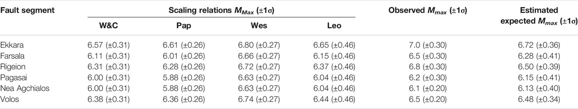
TABLE 3. Estimated Mmax and its ±1σ as obtained from the Wells and Coppersmith (1994; W&C), Papazachos et al. (2004; Pap), Wesnouskly (2008; Wes), and Leonard (2010; Leo) scaling relations for each of the six segments of the Southern Thessaly Fault Zone, along with the observed Mmax values (also listed in Table 1) used for the final estimation of the Mmax. The final estimates and their corresponding error (last column) using the modified version of Pace et al. (2016) method are also given.
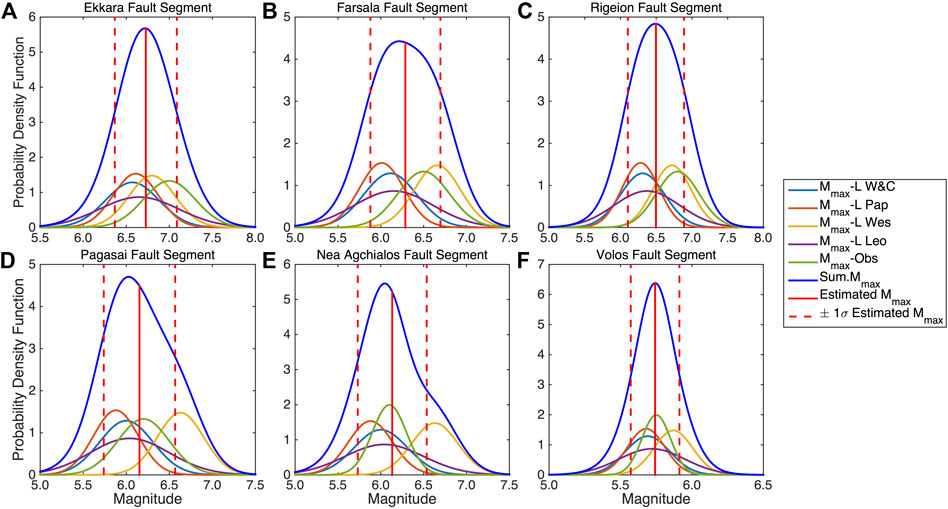
FIGURE 2. Probability density functions considering the normal distribution with mean value and standard deviation, the estimated Mmax, and its corresponding ±1σ as resulted from the (Wells and Coppersmith, 1994; light blue lines), (Papazachos et al., 2004; orange lines), (Wesnousky, 2008; yellow lines), and (Leonard 2010; magenta lines) scaling relations for normal faults using the fault segment length as input for each of the six segments of the Southern Thessaly Fault Zone. The green curves represent the normal distribution accrued from the observed Mmax and its ±1σ based on the past strong earthquakes that occurred per segment. Blue curves depict the summed probability functions resulted from the combination of both scaling densities, along with the observational ones. The central values and their corresponding ±1σ of the summed densities after the application of the Gaussian fit are shown with solid and dashed red lines, respectively.
A general remark concerning the estimates of the scaling relations is that Wesnousky’s (2008) relation returns the largest values of Mmax than the other 3, whose values are quite similar. For example, the Mmax for the Ekkara fault segment equals to 6.80 with Wesnousky’s (2008) relation, whereas the corresponding values using the Wells and Coppersmith 1994, Papazachos et al. 2004, and Leonard (2010) relations are equal to 6.57, 6.61, and 6.65, respectively. This fact slightly affects the +1σ part of the summed probability density (blue lines) in the cases of the Pagasai (Figure 3D) and Nea Agchialos (Figure 3E) fault segments.
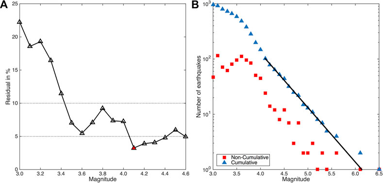
FIGURE 3. Completeness magnitude, Mc, estimation through the GFT method for the Southern Thessaly Fault System during the period 1970–2020. (A) Residual in percentiles as function of the minimum magnitude bin of the observed catalog. Red triangle indicates the bin with residual below 5%. (B) Frequency-Magnitude Distribution (FMD) of incremental (red squares) and cumulative (blue triangles) number of the earthquakes. Straight black line represents the part of FMD above Mc.
The final estimates of Mmax, resulted from the Gaussian fit of the summed density curves, show that the maximum expected magnitude values are slightly lower (but inside the +1σ confidence interval) than the observational ones in the cases of Ekkara (Mmax_exp = 6.72 instead of Mmax_obs = 7.0), Farsala (Mmax_exp = 6.28 instead of Mmax_obs = 6.5) and Rigeion (Mmax_exp = 6.50 instead of Mmax_obs = 6.8) fault segments. The estimates for Pagasai, Nea Agchialos, and Volos fault segments equal to Mmax_exp = 6.15, Mmax_exp = 6.13, and Mmax_exp = 6.48, respectively, are in very good agreement with the observed ones (Mmax_obs = 6.2, Mmax_obs = 6.1, and Mmax_obs = 6.5, respectively).
In summary, the maximum expected magnitude evaluation using the estimates from scaling laws and constrained by the observed Mmax, show the possible seismic potential of each fault segment. Some differences between the observed and the expected M values could possibly be related with some overestimation of the observed ones, due to the fact that these earthquakes occurred in the early instrumental period.
Simulator Algorithm Outline
The current simulation application is based on the algorithm developed and evolutionary improved by Console et al. 2015; Console et al. 2017; Console et al. 2018a; Console et al. 2020, where the main principles are analyzed in detail. In this section, a brief outline is presented about its main principles along with the improvement of the present version. The simulator algorithm comprises several physical constraints, including the geometry and the long-term slip rates of each segment of the 3-D fault model. Each fault segment is modeled as a quadrilateral plane source, onto which a normal grid of squared cells is superimposed. The long-term slip rate is distributed uniformly within a certain fault segment and could vary from one segment to the other. Each cell is initially assigned with a stress value taken from a random distribution, which then increases with time due to the slow tectonic loading in terms of a backslip model. The nucleation process is implemented by the contribution of the Rate and State Constitutive Law of Dieterich 1994, leading to a probabilistic manner of nucleation (Console et al., 2020).
Specifically, the seismicity rate, R, in each cell is calculated by:
where r is the reference seismicity rate of each cell (defined as the seismicity rate R when ΔCFF = 0), ΔCFF is the change in Coulomb Failure Function due to the coseismic slip of previous earthquakes, Ασ is the constitutive parameter describing the response of the friction to a rate change caused by a stress step change (Toda and Stein, 2003), Δt is the time elapsed after the stress change on a given cell, and γ0 is the inverse of the reference tectonic stressing rate,
where Δτ is the shear stress change in the slip direction, Δσn is the normal stress change, positive for extension normal to the observational fault plane, and μ′ is the apparent coefficient of friction (Rice, 1992).
After the nucleation initiation, the strength of neighboring cells is reduced according to a constant value multiplied by the square root of the number of initially ruptured cells, resembling a weakening mechanism and promoting the growth of the rupture. The expansion of each rupture is limited by a factor equal to a given number of times the width of the fault segment, discouraging the rupture propagation over long distances. Rupture growth and termination are controlled by two free parameters in the algorithm, the Strength Reduction (S-R) coefficient and the Aspect Ratio (A-R), referring to the fault weakening and the discouragement of the rupture propagation over long distances, respectively.
During the coseismic stage of the process, the stress is decreasing by a constant stress drop, Δp (e.g., Δp = 3 MPa) in every cell that participates in the rupture, while in the surrounding cells the stress changes are given by the Eq. 2. A given cell is allowed to rupture more than once in the same event, when it is ruptured with a constant stress drop but with only a moderate amount of slip.
A rupture terminates when there are no more cells inside the searched area, in which the stress exceeds their strength. Coulomb stress changes also contribute to the interactions among the causative and receiving segments, allowing the expansion of a rupture to neighboring fault segments, which are located within a certain maximum distance (e.g., 5 km). This feature of the algorithm represents the ability of fault interactions to possibly produce fault linkage and coalescence phenomena, resulting in large earthquakes due to the simultaneous rupture of more than one segment (Scholz, 2019).
A critical point that affects the results of the simulation procedure is the input values of the three free parameters. The influence of the two of them, the S-R and A-R, was already analyzed by Console et al. (2015, 2017, 2018a). The Strength-Reduction coefficient (S-R) mainly controls the ratio between the number of small to large events. Small values of S-R produce simulated catalogs with much fewer large events than the large S-R values and visa versa. The effect of the Aspect-Ratio (A-R) value is mainly related with the maximum magnitude, not with the total number of events nor with the b-value of the simulated catalogs. Additionally, the effect of the product Aσ of the Rate and State law is mainly related with the probability of event’s nucleation from the stress change due to the coseismic slip of previous events (Console et al., 2020).
Application of the Simulator to the Southern Thessaly Fault System
The six fault segments of the fault model are rectangular planes, divided into 0.75 × 0.75 km squared cells (Table 2 and Figure 1C). The 60% of the geodetically estimated slip, the values of rigidity, μ, and stress drop, Δp, equal to 40 GPa and 4 MPa, respectively, are considered for the simulator application. The minimum magnitude generated by the simulator is selected to be equal to 4.1 (Mw = 4.1), which corresponds to a two cells rupture.
An important step during the application of the simulator algorithm is the selection of the Aσ, S-R, and A-R free input parameters. This step is very crucial because the final simulated catalog will be affected by their influence in terms of the total number of event and the ratio between the number of small to moderate and large earthquakes (effects of nucleation and fault weakening, related with the values of Aσ and S-R). The maximum magnitude that the simulator generates will also be influenced by the effect of the value of A-R. A wide range of Aσ values are reported, ranging from 0.0012 to 0.6 MPa, obtained from different earthquake sequences (Harris, 1998; Harris and Simpson, 1998). Mangira et al. 2020 tested values ranging between 0.04 and 0.09 MPa in the Central Ionian Islands (Greece), with a value equal to Aσ = 0.06 MPa found to be the most appropriate. Console et al. 2020 used values between 0.01 and 1.0 Mpa concluding Aσ = 0.05 MPa for Central Italy. Since the value of the product Aσ is not fixed, a range from 0.01 to 0.04 MPa with a step of 0.005 MPa is selected to be tested in this study [Aσ = (0.01 MPa–0.04 MPa)].
The relevant knowledge about the mechanism of fault weakening is based in indirect observations, such as past seismicity, and consequently is mainly undetermined A range of S-R values are tested, starting from a value of 0.1, which represents strong faults, and with a step of 0.05 up to the value 0.3, in which the weakening is enhanced [S-R = (0.1–0.3)]. The third parameter, A-R, is assigned after testing it for values equal to 2, 3, and 4, in accordance with the dimensions of the six segments. The effort for testing all possible values of the three free parameters resulted in 105 combinations stemming from the considered value ranges (Supplementary Appendix B1). The duration of each simulation is selected to be equal to 10 kyr with a warm-up period of 2 kyr, which were not taken into account in each final simulated catalog.
Each triplet of input parameters yielded a simulated catalog with different total number of events, maximum magnitude, and b-values. The number of events ranges from 9,309 to 40,056, whereas the b-values are fluctuated between 0.92 and 1.50 (Supplementary Appendix B1) affected by the different values of Strength-Reduction coefficient. Maximum magnitude is found to be between 6.6 and 6.8 because of the different Aspect-Ratio values, in good agreement with the maximum expected magnitude for each fault segment as obtained from the scaling relations (Table 3).
The selection of the most representative simulated catalog is made after comparison with observational data. The observational data are taken from the instrumental catalog of Geophysics Department at the Aristotle University of Thessaloniki, 1981 (http://geophysics.geo.auth.gr/ss), based on the recordings of the Hellenic Unified Seismological Network (HUSN), and include all the available Mw ≥ 3.0 earthquakes from 1970 to 2020. The complete magnitude of this catalog is investigated with the application of the Goodness of Fit method (GFT; Wiemer and Wyss, 2000), considering the 95% confidence level of residuals (Figure 3A), and was found to equal Mc = 4.1, with 102 earthquakes (Figure 3B). The maximum likelihood estimate (Aki, 1965) gave b = 0.99, and the parameter α equals α = 6.05. A remarkable point arising from the FMD is the limited number of moderate to large earthquakes (5.7 ≤ Mw ≤ 6.1), implying the lack of the corresponding causative activated faults.
The comparison is implemented by assessing the performance of each simulated catalog against the observational one via the application of two non-parametric statistical tests, namely the two sample Kolmogorov—Smirnov (KS2) (Stephens, 1974) and the Wilcoxon Rank-Sum (WR-S) (Wilcoxon, 1945; Mann and Whitney, 1947), at a significance level equal to α = 0.05. Specifically, the cumulative earthquake number Ni of a certain simulated catalog for each magnitude bin divided by the corresponding period (Ni/period, in years) is compared with the corresponding observations, under the null hypothesis that the two rates come from the same population against the alternative hypothesis that they come from different populations at a given significance level, α.
The two sample K-S test is a non-parametric goodness of fit test, which compares the differences between the empirical cumulative distribution functions (ecdf), F (10) and G (x), of two samples under the null hypothesis. The statistic of the test is defined as:
The Wilcoxon Rank-Sum test compares two independent random variables, F and G, with sample sizes m and n, respectively, under the null hypothesis that the two samples come from the same distribution, similarly with the Mann-Whitney U-test. The samples are combined and ranked. The Wilcoxon statistic, T, is calculated from the sum of the ranks according to:
and
The number of times that Fi > Gj is in an ordered arrangement, so the Mann-Whitney statistic U is defined as:
where
and
The decision of rejecting or not the null hypothesis is based on the p-value returned by the test, compared with the significance level. If p-value is greater than α (p-value > α) then the null hypothesis can not be rejected. On the contrary, if p-value is lower than α (p-value < α) the null hypothesis can be rejected.
The results of the two statistical tests are shown in Supplementary Appendix B1 and Figure 4 in terms of their corresponding p-values, evidencing that in all cases their values are larger than the significance level, except for one case of the Wilcoxon Rank-Sum test, in which the p-value is equal to 0.032 (Simulation 90; Supplementary Appendix B1 and Figure 4). More specifically, the p-values of the KS2 test range from 0.051 to 0.685, and those of WR-S between 0.032 and 0.630. Ideally, the best performed simulated catalog would be the one with the sufficiently largest p-values in both tests. The current results evidence a large number of candidate simulated catalogs as the best performed, since their p-values are quite large in both tests in respect to the others.
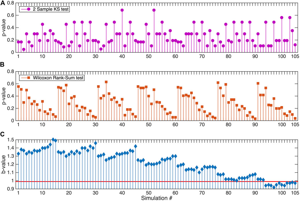
FIGURE 4. Calculated p-values of the two Sample Kolmogorov-Smirnov (A) and the Wilcoxon Rank-Sum (B) tests for the 105 simulated catalogs at 0.05 level of significance (α = 0.05). The b-values (C) of each simulated catalog (blue stems) are also presented vs. the observational catalog’s one (solid red line).
From a statistical point of view, each one of the simulated catalogs 19, 34, 52, 79, and 94 with values of free parameters (Ασ/S-R/A-R) equal to 0.015 MPa/0.15/2, 0.02 MPa/0.15/2, 0.025 MPa/0.2/2, 0.035 MPa/0.15/2, and 0.04 MPa/0.15/2, respectively, could be considered as the best performed, since their calculated p-values (Supplementary Appendix B1 and Figure 4) are both large enough (e.g. p-values > 0.5) and quite close to each other. Four out of the five triplets showed a clear better performance of the values of S-R = 0.15 and A-R = 2. Simulation 52 (0.025 MPa/0.2/2) results in slightly higher p-values than the others (0.685 and 0.503 in KS2 and WR-S tests, respectively), but these results must be treated with caution before the final decision due to the sensitivity of statistical tests.
On the other hand, the best performed simulated catalog must also be representative in terms of the physical properties of the observational catalog, as expressed by the observed seismicity. The comparison among the calculated b-values of the simulated catalogs against the observational catalog, could be a reliable additional index for the final selection. The b-values of the simulated catalogs 19, 34, 52, and 94 are found to be equal to 1.30 (bsim19 = 1.30), 1.25 (bsim34 = 1.25), 1.20 (bsim52 = 1.20), and 0.94 (bsim94 = 0.94), respectively. These values considerably differ from the value of the observational catalog, which is equal to 0.99 (bobs = 0.99). The b-value of the simulation 79 equals to 1.02 (bsim79 = 1.02) and is the one with the least difference in respect to the bobs. It should be mentioned at this point that there are additional simulated catalogs with b-values close to the bobs (eg, simulated catalogs 83 and 104 with bsim83 = 1.00 and bsim104 = 0.98, respectively; Figure 4C) but their statistical performance is poor.
Based on the above results, the simulated catalog 79 (yellow line in Figure 5) is considered as the best performed one in respect with the observed seismicity, identifying the catalog from which further recurrence time analysis will be accomplished.
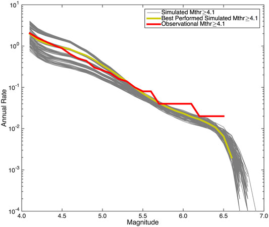
FIGURE 5. Summary of annual occurrence rates of the 105 simulated catalogs (gray lines), using different combinations of the free input parameters (Ασ, S-R, A-R; Supplementary Appendix A1). Annual occurrence rates of the best performed simulated catalog (Simulation 79; Ασ = 0.035 MPa, S-R = 0.15, A-R = 2) is represented by the yellow line, and the rates of the observational catalog with the red line.
The most representative simulated catalog is the one with Ασ = 0.035 MPa, S-R = 0.15, and A-R = 2, consisting of 19,740 events with Mw ≥ 4.1 with a duration of 10 kyrs. The largest magnitude of the simulated catalog is equal to 6.6 (Mw_max = 6.6), which is considerably smaller than both the maximum observed magnitudes equal to 7.0 and 6.8 that occurred in the Ekkara and Rigeion fault segments. The maximum expected magnitude of this catalog agrees well with the maximum expected magnitude yielded by the empirical relations analysis. These discrepancies among the maximum observed and simulated magnitudes could be explained with the fact that the 1954 Sofades (Mw = 7.0) and the 1957 Rigeion (Mw = 6.8) earthquakes belong to the early instrumental period and their magnitudes could possibly have beenoverestimated, as already said. Looking at the ISC-GEM instrumental earthquake catalog, the estimated magnitudes of these events are equal to Mw = 6.66 and Mw = 6.40, respectively, in very good agreement with the largest magnitude estimated in the simulated catalog. The comparison among the maximum expected magnitudes and the simulated magnitudes for single segment ruptures (Table 4) allow to accept that this simulated catalog represents quite accurately the seismicity in the study area.
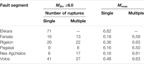
TABLE 4. Summary of single and multiple ruptures for the Mthr ≥ 6.0 for each of the six segments of the Southern Thessaly Fault Zone along with their maximum magnitude values obtained from the best performing 10 kyr simulated catalog (Simulation 79; Ασ = 0.035 MPa, S-R = 0.15, A-R = 2).
Strong (Mw ≥ 6.0) Earthquakes Occurrence and Recurrence Modeling
The main purpose of the simulation application is the provision of an earthquake catalog of both long duration and seismicity physical properties, appropriate for investigating the recurrence behavior of strong events in each fault segment of STFZ after fulfilling a set of criteria, that must be specified. Firstly, the minimum magnitude threshold above which the strong earthquakes will be considered a characteristic one, must be specified. Considering the observed strong events that occurred per segment (Figure 1) and their magnitude uncertainties (Table 1), along with their dimensions, a unique magnitude threshold equal to 6.0 (Mthr ≥ 6.0), corresponding to a group of at least 182 ruptured cells, is adopted.
Further, the contribution of each segment in a single earthquake must be specified. Each earthquake satisfying the first criterion is initially assigned to the segment in which the nucleation starts. Moreover, an additional fault segment could also participate with many ruptured cells in the same earthquake. In this way, if the number of ruptured cells of another segment are at least 75% of the total number of its cells (in other words, the rupture covers more than 75% of the segment’s area) or if they exceed the minimum number of cells as defined previously, then this segment is also assigned to the respective earthquake.
Considering these criteria, 254 ruptures in total are reported in the simulated catalog. Out of them, 169 earthquakes are related with single segment ruptures and 85 are multi segmented ruptures during the 10 kyr of the simulation. The latter number of ruptures can be separated into 38 pairs of simultaneously failed segments and three triplets of multiple ruptures. From the analysis of the ruptures per segment (Figure 6), some interesting features are observed. The Ekkara segment is the only one that ruptured alone because it is located in the southwest boundary of STFZ, and it is rather isolated from the other segments. The other five segments (Farsala, Rigeion, Pagasai, Nea Agchialos, and Volos) participate in both single and multiple ruptures with values of maximum magnitude around 6.6 (Table 4).
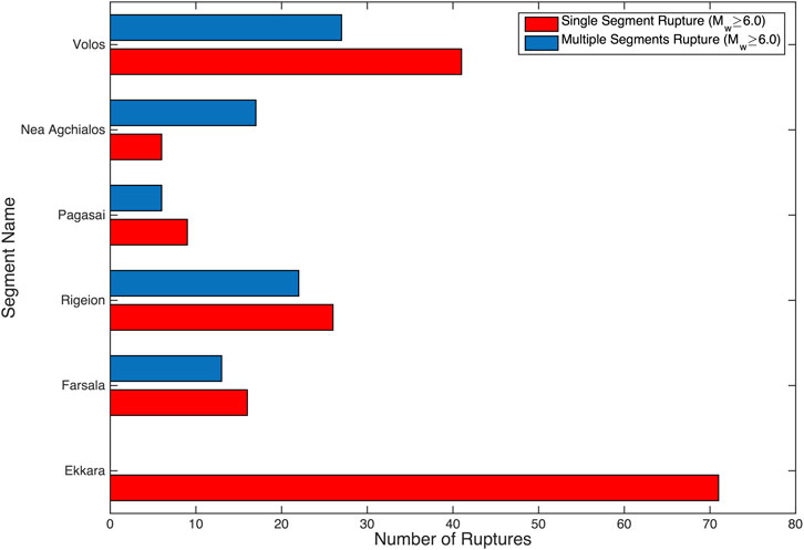
FIGURE 6. Number of both single (red bars) and multiple (blur bars) ruptures of each segment of the Southern Thessaly Fault Zone obtained from the best performed simulated catalog for the Mthr ≥ 6.0 characteristic earthquake magnitude threshold.
It is worth mentioning that the simulated catalog includes earthquakes in which more than segment has failed. An example is illustrated in Figure 7 for the first 2 kyr of the simulation and all the resulted multisegmented ruptures are given in Table 5. The main pattern of the two segment ruptures is that the neighbor fault segments are simultaneously failed in one earthquake, like the cases of Farsala–Rigeion and Nea Agchialos—Volos ones. There are some cases in which one segment of the northern group ruptured simultaneously with one from the southern group (e.g., the Pagasai—Volos ruptures), and in which the ruptured segments resulted in individual earthquakes with different magnitudes very close in time (e.g. within few seconds), as happened with Rigeion and Pagasai fault segments, that ruptured within a few seconds with magnitudes equal to Mw = 6.3 and Mw = 6.2, respectively (red ellipse in Figure 7).
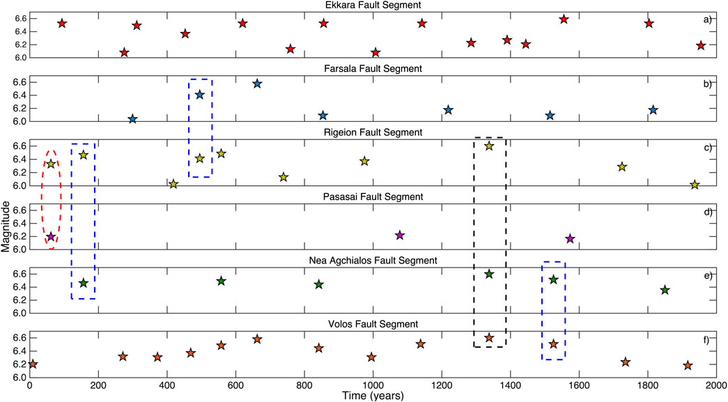
FIGURE 7. Snapshot of the first 2 kyr temporal distribution of the Mw ≥ 6.0 earthquakes of the best performed simulated catalog. Blue boxes indicate some of the combinations of the two segment ruptures, while the black one indicates one of the three cases of three segment ruptures. The red ellipse depicts a case of two individual fault segments ruptures (Mw = 6.3 for Rigeion fault segment and Mw = 6.2 for Pagasai fault segment) almost at the same time.
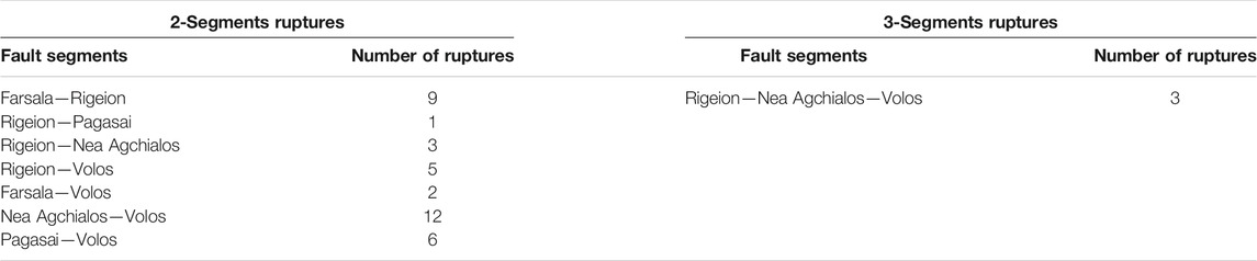
TABLE 5. Number of 2 and 3 segments’ multiple ruptures for all the combinations of the participating fault segments of the Southern Thessaly Fault Zone.
An illustrated example of the state of stress at a certain time illustrates the stress evolution in the six segments of STZF (Figure 8). The snapshot is selected to depict the state of stress at t = 1,336.338 years, when the Rigeion, Nea Agchialos, and Volos fault segments ruptured simultaneously (black dashed box of Figure 7), resulting in a Mw = 6.6 earthquake. Stress values are rather high (warm colors) within the cells of each fault segment that participate in the rupture (Figure 8). One additional remark derived from Figure 8 is that the stress values of the Pagasai fault segment are also high, indicating that the Pagasai fault segment is also close to a failure. This latter fact was confirmed with a single segment rupture of Pagasai fault segment at t = 1,574.264 years, resulting in a Mw = 6.2 earthquake.
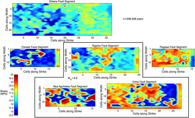
FIGURE 8. The state of stress (in MPa) in the six fault segments of STFZ at time t = 1,336.338 years, when the Rigeion, Nea Agchialos, and Volos fault segments ruptures simultaneously (black polygon), resulting in a Mw = 6.6 earthquake. The stress value on each cell is depicted with the color bar, ranging from 14.5 MPa (dark blue) to 20 MPa (dark red).
To study the earthquakes’ recurrence behavior in each fault segment, the mean recurrence time, Tr, along with its standard deviation (σ) and the corresponding coefficient of variation (Cv) are calculated (Table 6). The mean Tr obtained for the Mthr ≥ 6.0 earthquakes of the simulation procedure varies from almost 140–673 years, depending on the segment’s long term slip rate values and interactions. The Ekkara, Farsala, Rigeion, and Volos segments exhibit lower values of Tr equal to 140.49, 350.92, 205.02, and 149.19, respectively, since their slip rates are slightly higher than the other ones. Pagasai and Nea Agchialos segments exhibit considerably less frequent strong earthquake occurrence. These two segments could likely be characterized as auxiliary ones, playing a supportive role in stress accumulation and rupture propagation. In all these cases, either for larger or intermediate mean Tr, the values of the coefficient of variation, which range between 0.36 and 0.62 (Table 6), show a quasi-periodic recurrence behavior with a slight trend to a less periodic one for the Pagasai and Nea Agchialos fault segments.
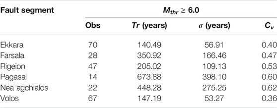
TABLE 6. Statistical parameters of the six segments of the Southern Thessaly Fault Zone as obtained from the best performing simulated catalog (Simulation 79; Ασ = 0.035 MPa, S-R = 0.15, A-R = 2) for the Mthr ≥ 6.0 adopted for the recurrence modeling.
In the next step of the recurrence modeling, two different approaches are adopted, aiming to assess whether the strong earthquake occurrence in each segment is better described by a memoryless Poisson process or by a renewal one. The Poisson process can be expressed by the exponential distribution with probability density function (pdf):
where Tr is the mean recurrence time in each data sample. The cumulative density function (cdf) of the exponential distribution is then defined as:
For modeling the strong earthquake occurrence as a renewal process, the Brownian Passage Time (BPT) distribution (Matthews et al., 2002) is used. The pdf of the BPT model is given by:
where Tr is also the mean recurrence time and α is the aperiodicity, which can be considered as analogous of the coefficient of variation of the normal distribution and represents the level of the randomness model taking values between 0 and 1 (0 ≤ α ≤ 1) to address the physical meaning of the recurrence of strong earthquakes, whereas the cdf is given by:
where
The comparison of the models is made in terms of their Akaike (Akaike, 1974) Information Criterion given by
where lnL and k stands for the value of the log-likelihood function and the number of parameters of the candidate model, respectively. The log-likelihood function of the Poisson process is defined by:
where N is the number of observations and t0 (N) is the occurrence time of the most remote event of the data sample, whereas the log-likelihood function of the BPT (or any other renewal model) is given by:
where Δt (j) is the interevent time between the jth and the jth 1 events and f (Δt) and F (t≤ Δt) are the pdf and cdf of the BPT distribution, respectively (Eqs 11, 12, respectively).
In this way, the two models are applied in each data sample of interevent times (ΔT) (Figure 9) and their corresponding log-likelihood values are calculated (Table 7). The results of these calculations reveal that the BPT model performs better than the Poisson model in all cases. In more detail, the BPT model is significantly better than the Poisson in the segments with larger numbers of observations, which are those with the lower values of Tr (Ekkara, Farsala, Rigeion, and Volos) and slightly better in the cases of large values of recurrence time and the larger values of Cv. This better performance of the renewal model adopted in this study suggests that an elastic rebound motivated behavior is more likely than the memoryless one.
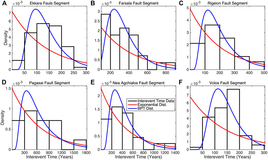
FIGURE 9. Probability density functions of Poisson (red line) and BPT (blue line) models for the interevent times of strong earthquakes with Mthr ≥ 6.0 for the Ekkara (A), Farsala (B), Rigeion (C), Pagasai (D), Nea Agchialos (E), and Volos (F) fault segments. Black boxes indicate the density values of each bin of interevent times.
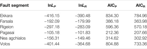
TABLE 7. Log-likelihood and AIC calculated values of the Poisson and the Renewal models for the six segments of the Southern Thessaly Fault Zone for the Mthr ≥ 6.0 adopted for the recurrence modeling. Subscripts P and R indicate the Poisson and the Renewal models, respectively.
Additionally, an analysis of the implications of the BPT model in the strong earthquakes’ occurrence per fault segment might be useful, highlighting also differences between the models in the forecasting of strong earthquakes in the near future. This analysis is based on the estimation of the hazard function, H (t), for both the BPT and the Exponential models using the estimated mean recurrence time, Tr, and the corresponding coefficient of variation as obtained from the statistical analysis of the simulated catalog (Table 5). The hazard function of a given distribution can be easily evaluated using its corresponding probability density, f(t), and cumulative density, F(t), functions as follows:
where S (t) is the survival function. Such an analysis is very useful for concluding future rupture scenarios. Specifically, the values of the hazard function or, in other words, the hazard rate, which is equivalent to the conditional probability estimate in a specific time span, could provide information on potential ruptures in the near future (Convertito and Faenza, 2014; Mangira et al., 2019).
In the current study, Eq. 18 is applied for both models (Eqs 9, 10 for the Exponential and Eqs 11, 12 for BPT models, respectively) for each of the six segments of STFZ. The estimated hazard functions are shown in Figure 10. Setting t = 0 as the occurrence date of the Mw ≥ 6.0 earthquake, it is derived that in all cases the values of the hazard function of the BPT model (blue lines) are very low soon after the occurrence of the earthquake and then they exhibit an increasing trend with time, taking its maximum value at some finite time close or soon after the mean recurrence time (black dashed lines).
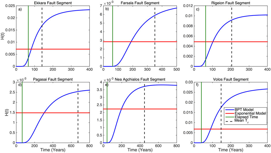
FIGURE 10. Hazard functions, h (t), for the Ekkara (A), Farsala (B), Rigeion (C), Pagasai (D), Nea Agchialos (E), and Volos (F) Fault SEgments according to the BPT renewal model (blue lines) against the memoryless exponential (red lines) one. Green lines represent the elapsed time since the last earthquake (t = 0), while the dashed black lines the mean Tr of the Mw ≥ 6.0 as obtained from the statistical analysis of the simulated catalog (Table 5) for each one of the six segments.
In the cases of low to intermediate aperiodicity (Ekkara Fault Segment; α = 0.40, Farsala Fault Segment; α = 0.47, Rigeion Fault Segment; α = 0.53 and Volos Fault Segment; α = 0.36), showing high occurrence probabilities late in the earthquake cycle, flattening of the hazard function curve is achieved soon after the recurrence time. In the cases of higher aperiodicity, namely the Pagasai and Nea Agchialos Fault segments with aperiodicity equal to α = 0.60 and α = 0.62, respectively, the maximum value is temporally closest to the mean recurrence time, yielding higher values earlier in the seismic cycle. In contrast, the Exponential model returns a constant hazard rate independently of both the mean recurrence time and the calculated elapsed time (until 01–01-2020; green lines) since the last event in each segment.
Considering these results, along with the better performance of the renewal BPT model as resulted from the values of the Information Criteria (Table 6), the elastic rebound motivated rupture scenarios is clearly supported. Taking into account this remark and focusing on the mean recurrence time, and the elapsed time in each case, one can conclude that all six segments are far from a future rupture. This fact can be explained by the short elapsed time since the last event per segment, very short for the stress to be rebuilt and culminate in the next strong earthquake. Specifically, the hazard rate is almost zero and considerably far from their maximum values in the cases of Farsala, Pagasai, Nea Agchialos, and Volos fault segments, whereas for the corresponding values of the Ekkara and Rigeion fault segments, both are at the increasing part of their curves but far enough from their mean recurrence times (about 74 and 142 years, respectively) and their pick values.
Discussion and Conclusion
The application of the physics-based simulator algorithm in the STFZ produced a simulated seismic catalog lasting 10 kyr and containing 19,760 events with Mw ≥ 4.1, from which the 254 corresponds with Mw ≥ 6.0. This large number of simulated ruptures provides the ability of a thorough study of their recurrence properties o, since the number of observed ones is very limited. In the four out of the six fault segments only one observation is available. For example, only one earthquake with Mw ≥ 6.0 is known to have occurred since 1700 in the Ekkara fault segment, which is the largest segment with the largest observed earthquake. The simulated catalog manages to resemble the observed seismicity successfully, as its b-value is very close with the value calculated from the observations.
Some mismatches are found between the maximum observed magnitude per segment and the one resulted by the simulation approach. These differences may be ascribed to the fact that the majority of strong earthquakes occurred in the study area in the early instrumental period, the magnitudes of which are possibly overestimated. Such cases are the magnitudes of the 1954 and 1958 earthquakes with Mw = 7.0 and Mw = 6.8 that occurred in the Ekkara and Rigeion segments, respectively. By assessing the ISC-GEM instrumental earthquake catalog, these earthquakes are found to be reported with magnitudes equal to Mw = 6.66 and Mw = 6.40, in agreement with those of the simulated catalog.
Emphasizing on the strong earthquakes, both single and multiple segment ruptures are found in the simulated catalog. The multiple segment ruptures can be distinguished into two and three segment ruptures, with the majority of them be composed of two segments. This fact could be ascribed to the similarity of their long-term slip rates that promotes the participation of more than one segment in simultaneous ruptures. This conclusion is in agreement with the study of Scholz 2019, who suggests that the fault synchronization and rupture jumping phenomena are more likely in segments with equal or similar slip rate values.
The mean recurrence time, Tr, for the selected magnitude threshold, Mthr_≥6.0 can be separated in to classes, depending on the fault segments. The four segments with larger areas (larger L and W), namely the Ekkara, Farsala, Rigeion, and Volos, exhibit relatively moderate Tr values ranging from 140 to 350 years and values of Cv revealing a high periodic occurrence (0.36 ≤ Cv ≤ 0.53). The other class includes the two fault segments of Pagasai and Nea Agchialos, whose mean recurrence times are quite large. This latter class of segments could probably be characterized as auxiliary, since these segments participate more frequently in multiple ruptures. A remarkable feature of these two segments is that they exhibit more aperiodic behavior with values of Cv around 0.6 (Table 6). This behavior could be explained by the fact that the reset of stress possibly results in a delay in the strong earthquake occurrence.
The application of the Poisson model against the BPT model in interevent times of earthquakes with Mthr_≥6.0 reveals a considerably better performance of the renewal BPT model than the memoryless Poisson model in all fault segments of the STFZ, which is in agreement with the elastic rebound theory (Reid, 1911, and a rather quasi-periodic recurrence behavior, as derived from the analysis of their hazard functions in combination with the elapsed time since the last event per segment. It should be mentioned that these results are independent from the algorithm itself, since its operates without any assumption related with the temporal occurrence of the earthquakes. As a consequence, the comparison among the statistical models are applied without a null hypothesis that could promote one model against the other.
Data Availability Statement
The raw data supporting the conclusions of this article will be made available by the authors, without undue reservation.
Author Contributions
CK has treated the data, applied the simulator algorithm and organized writing of the paper RC has developed the simulator algorithm, checked the application, interpreted the data and contributed to the writing of the paper EP has selected the study area and data, supervised the application, interpreted the data and contributed to the writing of the paper MM supervised the application, interpreted the data and contributed to the writing of the paper VK supervised the application, interpreted the data and contributed to the writing of the paper. All the authors contributed to the article and approved the submitted version.
Funding
The first author would like to acknowledge the financial support of the project “HELPOS—Hellenic System for Lithosphere Monitoring” (MIS 5002697) which is implemented under the Action “Reinforcement of the Research and Innovation Infrastructure”, funded by the Operational Programme “Competitiveness, Entrepreneurship, and Innovation” (NSRF 2014-2020) and co-financed by Greece and the European Union (European Regional Development Fund).
Conflict of Interest
The authors declare that the research was conducted in the absence of any commercial or financial relationships that could be construed as a potential conflict of interest.
Acknowledgments
We greatly appreciate the editorial assistance of Prof. B. Presti, as well as the constructive comments of Dr. J. Woessner and Dr. M. Mesimeri that contributed to the improvement of the manuscript. The historical and instrumental earthquake catalogs of the Geophysics Department of the Aristotle University of Thessaloniki (http://geophysics.geo.auth.gr/ss) and the instrumental ISC-GEM catalog provided by the International Seismic Centre, 2019http://www.isc.ac.uk/iscgem/index are used in this study. The maps and graphs are generated using the GMT software (Wessel et al., 2013) and MATLAB software (http://www.mathworks.com/products/matlab). NOA active fault database (version 3.0; doi:10.5281/zenodo.4304613) is accessible from https://noa-beyondapps.maps.arcgis.com/. Fault plane solutions’ data used in this paper came from resources listed in the References Section. Geophysics Department Contribution 942.
Supplementary Material
The Supplementary Material for this article can be found online at: https://www.frontiersin.org/articles/10.3389/feart.2021.596854/full#supplementary-material.
References
Akaike, H. (1974). A new look at the statistical model identification. IEEE Trans. Autom. Control, AC- 19, 716–723. doi:10.1109/tac.1974.1100705
Aki, K. (1965). Maximum likelihood estimation of b in the formula log n = a – bm and its confidence limits. Bull. Earthq. Res. Inst. Tokyo Univ. 43, 237–239.
Ambraseys, N. (2009). Earthquakes in eastern mediterranean and the Middle East: a multidisciplinary study of 2000 Years of seismicity. Cambridge, U.K.: Cambridge University Press, 947.
Ambraseys, N. N., and Jackson, J. A. (1990). Seismicity and associated strain of central Greece between 1890 and 1988. Geophys. J. Intell. 101, 663–708. doi:10.1111/j.1365-246x.1990.tb05577.x
Argyrakis, P., Ganas, A., Valkaniotis, S., Tsioumas, V., Sagias, N., and Psiloglou, B. (2020). Anthropogenically induced subsidence in Thessaly, central Greece: new evidence from GNSS data. Nat. Hazards 102, 179–200. doi:10.1007/s11069-020-03917-w
Aristotle University of Thessaloniki (1981). Aristotle University of Thessaloniki seismological network. Inter. Fed. Dig.Seis. Net. doi:10.7914/SN/HT
Biasi, G. P., Langridge, R. M., Berryman, K. R., Clark, K. J., and Cochran, U. A. (2015). Maximum-likelihood recurrence parameters and conditional probability of a ground-rupturing earthquake on the southern Alpine fault, South Island, New Zealand. Bull. Seismol. Soc. Am. 105, 96–106. doi:10.1785/0120130259
Biasi, G. P., and Thompson, S. C. (2018). Estimating time-dependent seismic hazard of faults in the absence of an earthquake recurrence record. Bull. Seismol. Soc. Am. 108, 39–50. doi:10.1785/0120170019
Caputo, R., and Pavlides, S. (1993). Late Caenozoic geodynamic evolution of Thessaly and surroundings (central-northern Greece). Tectonophysics 223, 339–362. doi:10.1016/0040-1951(93)90144-9
Caputo, R., and Pavlides, S. (2013). The Greek Database of seismogenic sources (GreDaSS), version 2.0.0: a compilation of potential seismogenic sources (Mw > 5.5) in the aegean region. doi:10.15160/unife/gredass/0200
Caputo, R. (1996). The active Nea Anchiale fault system (Central Greece): comparison of geological, morphotectonic, archaeological and seismological data. Ann. Geofisc. 39, 557–574.
Christophersen, A., Rhoades, D. A., and Colella, H. V. (2017). Precursory seismicity in regions of low strain rate: insights from a physical-based earthquake simularor. Geophys. J. Int. 209, 1513–1525. doi:10.1093/gji/ggx104
Console, R., Carluccio, R., Papadimitriou, E., and Karakostas, V. (2015). Synthetic earthquake catalogs simulating seismic activity in the Corinth Gulf, Greece, fault system. J. Geophys. Res. 120, 326–343. doi:10.1002/2014JB011765
Console, R., Chiappini, M., Minelli, L., Speranza, F., Carluccio, R., and Greco, M. (2018b). Seismic hazard in southern Calabria (Italy) based on the analysis of a synthetic earthquake catalog. Acta Geophys. 66, 931–943. doi:10.1007/s11600-018-0181-7
Console, R., Murru, M., Vannoli, P., Carluccio, R., Taroni, M., and Falcone, G. (2020). Physics-based simulation of sequences with multiple mainshocks in Central Italy. Geophys. J. Int. 223, 526–542. doi:10.1093/gji/ggaa300
Console, R., Nardi, A., Carluccio, R., Murru, M., Falcone, G., and Parsons, T. (2017). A physics-based earthquake simulator and its application to seismic hazard assessment in Calabria (Southern Italy) region. Acta Geophys. 65, 243–257. doi:10.1007/s11600-017-0020-2
Console, R., Vannoli, P., and Carluccio, R. (2018a). The seismicity of Central Apennines (Italy) studied by means of a physics-based earthquake simulator. Geophys. J. Int. 212, 916–929. doi:10.1093/gji/ggx451
Convertito, V., and Faenza, L. (2014). “Earthquake recurrence,” in Encyclopedia of earthquake engineering. Editors M. Beer, I. A. Kougioumtzoglou, E. Patelli, and I. Siu-Kui Au (Berlin, Germany: Springer), 1–22. doi:10.1007/978-3-642-36197-5-236-1
Davis, R., England, P., and Parsons, B. (1997). Geodetic strain of Greece in the interval 1892-1992. J. Geophys. Res. 102 (24), 571–624. doi:10.1029/97jb02378
Dieterich, J. H. (1994). A constitutive law for rate of earthquake production and its application to earthquake clustering. J. Geophys. Res. 99, 2601–2618. doi:10.1029/93jb02581
Drakos, A., Stiros, S. C., and Kiratzi, A. A. (2001). Fault parameters of the 1980 (Mw 6.5) Volos, Central Greece, earthquake from inversion of repeated leveling data. Bull. Seismol. Soc. Am. 91 (6), 1673–1684. doi:10.1785/0120000232
Ellsworth, W. L., Matthews, M. V., Nadeau, R. M., Nishenko, S. P., Reasenberg, P. A., and Simpson, R. W. (1999). A physically based earthquake recurrence model for estimation of long-term earthquake probabilities. U.S. Geol. Surv. Open-File Rept., 99–522.
Field, E. H. (2015). Computing elastic-rebound-motivated earthquake probabilities in unsegments fault models: a new methodology supported by physics-based simulators. Bull. Seismol. Soc. Am. 105, 544–559. doi:10.1785/01201140094
Fitzenz, D. D. (2018). Conditional probability of what? Example of nankai interface in Japan. Bull. Seismol. Soc. Am. 108 (6), 3169–3179. doi:10.1785/0120180016
Galanakis, D., Pavlidis, S., and Mountrakis, D. (1998). Recent brittle tectonic in almyros-pagasitikos, Maliakos, N. Euboea and pilio. Bull. Geol. Soc. Greece XXXXII/1, 263–273.
Ganas, A., Oikonomou, I. A., and Tsimi, C. (2013). NOAFAULTS: a digital database for active faults in Greece. Bull. Geol. Soc. Greece 47 (2), 518–530. doi:10.12681/bgsg.11079
Goldsworthy, M., Jackson, J., and Haines, J. (2002). The continuity of active faults systems in Greece. Geophys. J. Int. 148, 596–618. doi:10.1046/j.1365-246x.2002.01609.x
Goldsworthy, M., and Jackson, J. A. (2000). Active normal fault evolution and interaction in Greece revealed by geomorphology and drainage patterns. J. Geol. Soc. Lond. 157, 967–981. doi:10.1144/jgs.157.5.967
Harris, R. A. (1998). Introduction to special section: stress triggers, stress shadows, and implications for seismic hazard. J. Geophys. Res. 103, 24. 346–24, 358. doi:10.1029/98JB01576/
Harris, R. A., and Simpson, R. W. (1998). Suppression of large earthquakes by stress shadows: a comparison of Coulomb and rate-and-state failure. J. Geophys. Res. 103, 24, 439–24,451. doi:10.1029/98JB00793
Hatzfeld, D., Ziazia, M., Kementzetzidou, D., Hatzidimitriou, P., Panagiotopoulos, D., Makropoulos, K., et al. (1999). Microseismicity and focal mechanisms at the western termination of the North Anatolian Fault and their implications for continental tectonics. Geophys. J. Int. 137, 891–908. doi:10.1046/j.1365-246x.1999.00851.x
Jenny, S., Goes, S., Giardini, D., and Kahle, H.-G. (2004). Earthquake recurrence parameters from seismic and geodetic strain rates in the eastern Mediterranean. Geophys. J. Intell. 157, 1331–1347. doi:10.1111/j.1365.246X.2004.02261.x
Mangira, O., Console, R., Papadimitriou, E., Murru, M., and Karakostas, V. (2020). The short-term seismicity of the Central Ionian Islands (Greece) studied by means of a clustering model. Geophys. J. Int. 220, 856–875. doi:10.1093/gji/ggz481
Mangira, O., Kourouklas, C., Chorozoglou, D., Iliopoulos, A., and Papadimitriou, E. (2019). Modeling the earthquake occurrence with time-dependent processes: a brief review. Acta Geophys. 67, 739–752. doi:10.1007/s11600-019-00284-4
Mann, H. B., and Whitney, D. R. (1947). On a test of whether one of two random variables is stochastically larger than the other. Ann. Math. Stat. 18 (1), 50–60. doi:10.1214/aoms/1177730491
McKenzie, D. (1972). Active tectonics of the mediterranean region. Geophys. J. Int. 30, 109–185. doi:10.1111/j.1365-246X.1972.tb02351.x
Mountrakis, D., Kilias, A., Pavlides, S., Zouros, N., Spyropoulos, N, Tranos, M., and Soulakelis, N. (1993). “Field study of the southern Thessaly highly active fault zone,” in Proc. 2nd Congr. Hellenic Geophys. Union, 2, 603-614.
Leonard, M. (2010). Earthquake fault scaling: relating rupture length, width, average displacement, and moment release. Bull. Seismol. Soc. Am. 100(5A). 1971–1988. doi:10.1785/0120090189
Muller, M. D., Geiger, A., Kahle, H.-G., Veis, G., Billiris, H., Paradissis, D., et al. (2013). Velocity and deformation fields in the North Aegean domain, Greece, and implications for fault kinematics, derived from GPS data 1993-2009, Tectonophysics, 597–598, 34–49. doi:10.1016/j.tecto.2012.08.003
Ogata, Y. (2002). Slip-size-dependent renewal process and Bayesian inferences for uncertainties. J. Geophys. Res. 107(B11). 2268. doi:10.1029/2001JB9000668
Pace, B., Visini, F., and Peruzza, L. (2016). FiSH: MATLAB Tools to turn fault data into seismic-hazard models. Seismol Res. Lett. 87, 374–386. doi:10.1785/0220150189
Papadimitriou, E., and Karakostas, V. (2003). Episodic occurrence of strong (Mw≥6.2) earthquakes in Thessalia area (central Greece). Earth Planet Sci. Lett. 215, 395–409. doi:10.1016/S0012-812X(03)00456-4
Papastamatiou, D., and Mouyaris, N. (1986). The earthquake of april 30, 1954, in Sofades (Central Greece). J. R. Astron. Soc. 87, 885–895. doi:10.1111/j.1365-246x.1986.tb01975.x
Papazachos, B. C., and Comninakis, P. E. (1971). Geophysical and tectonic features of the Aegean arc. J. Geophys. Res. 76, 8517–8533. doi:10.1029/jb076i035p08517
Papazachos, B. C., and Comninakis, P. E. (1970). Geophysical features of the Greek island arc and eastern Mediterranean ridge. Com. Ren. Des Sceances la Conf. Reunie a Madrid 16, 74–75.
Papazachos, B. C., Hatzidimitriou, P. M., Karakaisis, G. F., Papazachos, C. B., and Tsokas, G. N. (1993). Rupture zones and active crustal deformation in southern Thessaly, central Greece. Boll. Geof. Teor. Appl. 139, 363–374.
Papazachos, B.C., Mountrakis, D.M., Papazachos, C.B., Tranos, M.D., Karakaisis, G.F., and Savvaidis, A.S., (2001). “The faults that caused the known strong earthquakes in Greece and surrounding areas during 5th century B.C. up to present,”in 2nd Conf. Earthq. Eng. Eng. Seism., September 2–30 2001, Thessaloniki, Greece, 17-26.
Papazachos, B. C., Panagiotopoulos, D. G., Tsapanos, T. M., Mountrakis, D. M., and Dimopoulos, G. Ch. (1983). A study of the 1980 summer seismic sequence in the Magnesia region of central Greece. J. R. Astron. Soc. 75, 155–168. doi:10.1111/j.1365-246x.1983.tb01918.x
Papazachos, B. C., Papadimitriou, E. E., Kiratzi, A. A., Papazachos, C. B., and Louvari, E. K. (1998). Fault plane solutions in the Aegean Sea and the surrounding area and their tectonic implications. Boll. Geof. Teor. App. 39, 199–218.
Papazachos, B. C., Scordilis, M. E., Panagiotopoulos, D. G., Papazachos, C. B., and Karakaisis, G. F. (2004). Global relations between seismic fault parameters and moment magnitude of earthquakes. Bull. Geol. Soc. Greece 36 (3), 1482–1489. doi:10.12681/bgsg.16538
Papazachos, G., Papazachos, C., Skarlatoudis, A., Kkallas, H., and Lekkas, E. (2016). Modelling macroseismic observations for historical earthquakes: the cases of the M=7.0, 1954 Sofades and M=6.8, 1957 Velestino events (central Greece). J. Seismol. 20, 151–165. doi:10.1007/s10950-015-9517-9
Perissoratis, C., Angelopoulos, I., Mitropoulos, D., and Michailidis, S. (1991). Surficial sediment map of the Aegean Sea floorScale 1:200,000. Athens: Pagasitikos sheet, IGME.
Reid, H. F. (1911). The elastic-rebound theory of earthquakes, Univ. Calif. Pub. Bull. Dept. Geol. Sci. 6, 413–444.
Rice, J. R. (1992). Fault stress states, pore pressure distributions, and the weakness of the San Andreas fault. In Fault mechanics and transport properties of rocks; a festschrift in honour of W. F. Brace. Editors B. Evans and T. Wong. San Diego, CA, USA: Academic Press, 475–503.
Richards-Dinger, K., and Dieterich, J. H. (2012). RSQSim earthquake simulator. Seismol Res. Lett. 83, 983–990. doi:10.1785/0220120105
Roberts, G. P., and Ganas, A. (2000). Fault-slip directions in central and southern Greece measured from striated and corrugated fault planes: comparison with focal mechanism and geodetic data. J. Geophys. Res. 105 (23). 443–462. doi:10.1029/1999jb900440
Roberts, G. P. (1996). Variations in fault slip directions along active and segmented normal fault systems. J. Struct. Geol. 18, 835–845. doi:10.1016/s0191-8141(96)80016-2
Robinson, R., and Benites, R. (1996). Synthetic seismicity models for the Wellington Region, New Zealand: implications for the temporal distribution of large events. J. Geophys. Res. 101 (27), 833–844. doi:10.1029/96jb02533
Robinson, R., Van Dissen, R., and Litchfield, N. (2011). Using synthetic seismicity to evaluate seismic hazard in the Wellington region, New Zealand. Geophys. J. Int. 187, 510–528. doi:10.1111/j.1365-246X.2011.05161.x
Rundle, J. B. (1988). A physical model for earthquakes. 2. Application to southern California. J. Geophys. Res. 93, 6255–6274. doi:10.1029/jb093ib06p06255
Sachs, M. K., Yikilmaz, M. B., Heien, E. M., Rundle, J. B., Turcotte, D. L., and Kellogg, L. H. (2012). Virtual California earthquake simulator. Seismol Res. Lett. 83, 973–978. doi:10.1785/0220120052
Scholz, C. H. (2019). The mechanics of earthquake and faulting. 3rd edn. Cambridge University Press, 504.
Schultz, K. W., Yoder, M. R., Wilson, J. M., Heien, E. M., Sachs, M. K., Rundle, J. B., et al. (2017). Parametrizing physics-based earthquake simulations. Pure Appl. Geophys. 174, 2269–2278. doi:10.1007/s00024-016-1428-3
Shaw, B. E., Milner, K. R., Field, E. H., Richards-Dinger, K., Gilchrist, J. J., Dieterich, J. H., et al. (2018). A physics-based simulator replicates seismic hazard statistics in California. Sci. Adv. 4 (8). doi:10.1126/sciadv.aau0688
Stephens, M. A. (1974). EDF statistics for goodness of fit and some comparisons. J. Am. Stat. Assoc. 64 (374), 730–737. doi:10.2307/2286009
Sykes, L. R., and Menke, W. (2006). Repeat times of large earthquakes: implications for earthquake mechanics and long-term prediction. Bull. Seismol. Soc. Am. 96, 1569–1596. doi:10.1785/0120050083
Toda, S., and Stein, R. S. (2003). Toggling of seismicity by the 1997 Kagoshima earthquake couplet: a demonstration of time-dependent stress transfer. J. Geophys. Res. 108 (B12). 2567. doi:10.1019/2003JB002527
Tullis, T. E. (2012a). Preface to the focused issue on earthquake simulators. Seismol Res. Lett. 83, 957–958. doi:10.1785/0220120122
Ward, S. N. (2012). ALLCALL earthquake simulator. Seismol Res. Lett. 83, 964–972. doi:10.1785/0220120056
Wells, D. L., and Coppersmith, K. J. (1994). New empirical relationships among magnitude, rupture length, rupture width, rupture area, and surface displacement. Bull. Seismol. Soc. Am. 84, 974–1002.
Wesnousky, S. G. (2008). Displacement and geometrical characteristics of earthquake surface ruptures: Issues and implications for seismic hazard analysis and the process of earthquake rupture. Bull. Seismol. Soc. Am. 98(4). 1609–1632. doi:10.1785/0120070111
Wessel, P., Smith, W. H. F., Scharroo, R., Luis, J., and Wobbe, F., (2013). Generic mapping tools: improved version released. EOS Trans. Am. Geophys. Union, 94, 409-410. doi:10.1002/2013eo450001
Wiemer, S., and Wyss, M. (2000). Minimum magnitude of completeness in earthquake catalogs: examples from Alaska, the western United States, and Japan. Bull. Seismol. Soc. Am. 90, 859–869. doi:10.1785/0119990114
Wilcoxon, F. (1945). Individual comparison by ranking methods. Biometrics 1 (6), 80–83. doi:10.2307/3001968
Keywords: strong earthquakes recurrence models, physics-based earthquake simulator, fault interaction, statistical analysis, southern Thessaly, Greece
Citation: Kourouklas C, Console R, Papadimitriou E, Murru M and Karakostas V (2021) Strong Earthquakes Recurrence Times of the Southern Thessaly, Greece, Fault System: Insights from a Physics-Based Simulator Application. Front. Earth Sci. 9:596854. doi: 10.3389/feart.2021.596854
Received: 20 August 2020; Accepted: 07 January 2021;
Published: 25 February 2021.
Edited by:
Debora Presti, University of Messina, ItalyReviewed by:
Jochen Woessner, Risk Management Solutions, SwitzerlandMaria Mesimeri, The University of Utah, United States
Copyright © 2021 Kourouklas, Console, Papadimitriou, Murru and Karakostas. This is an open-access article distributed under the terms of the Creative Commons Attribution License (CC BY). The use, distribution or reproduction in other forums is permitted, provided the original author(s) and the copyright owner(s) are credited and that the original publication in this journal is cited, in accordance with accepted academic practice. No use, distribution or reproduction is permitted which does not comply with these terms.
*Correspondence: Eleftheria Papadimitriou, cml0c2FAZ2VvLmF1dGguZ3I=