 V. A. Pilipenko
 E. N. Fedorov2
94% of researchers rate our articles as excellent or good
Learn more about the work of our research integrity team to safeguard the quality of each article we publish.
Find out more
ORIGINAL RESEARCH article
Front. Earth Sci., 27 January 2021
Sec. Atmospheric Science
Volume 8 - 2020 | https://doi.org/10.3389/feart.2020.619227
This article is part of the Research TopicAtmospheric ElectricityView all 12 articles
Variations of vertical atmospheric electric field Ez have been attributed mainly to meteorological processes. On the other hand, the theory of electromagnetic waves in the atmosphere, between the bottom ionosphere and earth’s surface, predicts two modes, magnetic H (TE) and electric E (TH) modes, where the E-mode has a vertical electric field component, Ez. Past attempts to find signatures of ULF (periods from fractions to tens of minutes) disturbances in Ez gave contradictory results. Recently, study of ULF disturbances of atmospheric electric field became feasible thanks to project GLOCAEM, which united stations with 1 sec measurements of potential gradient. These data enable us to address the long-standing problem of the coupling between atmospheric electricity and space weather disturbances at ULF time scales. Also, we have reexamined results of earlier balloon-born electric field and ground magnetic field measurements in Antarctica. Transmission of storm sudden commencement (SSC) impulses to lower latitudes was often interpreted as excitation of the electric TH0 mode, instantly propagating along the ionosphere–ground waveguide. According to this theoretical estimate, even a weak magnetic signature of the E-mode ∼1 nT must be accompanied by a burst of Ez well exceeding the atmospheric potential gradient. We have examined simultaneous records of magnetometers and electric field-mills during >50 SSC events in 2007–2019 in search for signatures of E-mode. However, the observed Ez disturbance never exceeded background fluctuations ∼10 V/m, much less than expected for the TH0 mode. We constructed a model of the electromagnetic ULF response to an oscillating magnetospheric field-aligned current incident onto the realistic ionosphere and atmosphere. The model is based on numerical solution of the full-wave equations in the atmospheric-ionospheric collisional plasma, using parameters that were reconstructed using the IRI model. We have calculated the vertical and horizontal distributions of magnetic and electric fields of both H- and E-modes excited by magnetospheric field-aligned currents. The model predicts that the excitation rate of the E-mode by magnetospheric disturbances is low, so only a weak Ez response with a magnitude of ∼several V/m will be produced by ∼100 nT geomagnetic disturbance. However, at balloon heights (∼30 km), electric field of the E-mode becomes dominating. Predicted amplitudes of horizontal electric field in the atmosphere induced by Pc5 pulsations and travelling convection vortices, about tens of mV/m, are in good agreement with balloon electric field and ground magnetometer observations.
The mutual fertilization of two geophysical disciplines—space physics and atmospheric electricity, has been rather low so far. This neglect is related to the fact that variations of the atmospheric electric field are commonly considered to be totally influenced by local meteorological processes. As a result, the magnetospheric community and atmospheric electricity community practically do not interact. In particular, in studies of waves and transients in the ultra-low-frequency (ULF) band (from mHz to Hz), the impact of magnetospheric disturbances on gradient of atmospheric potential (i.e., vertical electric field Ez) was commonly neglected, besides a few studies mentioned below.
Electromagnetic waves in the atmosphere, between the conductive layers of the bottom ionosphere and earth’s surface, can be decomposed into the magnetic H-mode (TE or THM mode) and electric E-mode (TH or TEM mode). Each mode has a specific partial impedance characterizing its interaction with the earth’s crust (Berdichevsky et al., 1971). The H-mode carries a vertical magnetic field disturbance, Bz, while the E-mode carries a vertical electric field disturbance, Ez. Upon modeling of magnetospheric MHD wave (Alfven (Hughes and Southwood, 1976) and fast compressional (Hamieri and Kivelson, 1991) modes) interaction with the ionosphere-atmosphere-ground system, the contribution of the E-mode is commonly neglected, so the ground response is believed to be produced by the H-mode only (Alperovich and Fedorov, 2007).
The E-modes are effectively excited in the ELF-VLF bands (e.g., Schumann resonances and sferics) by lightning electric discharges. Does the E-mode contribute also in the electromagnetic field of ULF waves? So far, there is no definitive answer to this question.
Apart from space physics applications, this problem is of key importance for magnetotelluric sounding (MTS) fundamentals. On the assumption that the incident ULF field is composed of a superposition of partial E- and H-modes, a new method of MTS, directional analysis, was developed by Chetaev (1970). This method is based on the premise that the spatial structure of ULF pulsations above a high-resistive crust does not meet the plane wave approximation and should be modeled as a horizontally propagating inhomogeneous plane wave with a complex wave vector (Dmitriev, 1970; Chetaev, 1985). According to this concept, the electric mode carrying a large vertical electric field/current in the air is a part of a primary wave. In this regard, verification of possible occurrences of Ez in the atmosphere in the ULF range is of fundamental importance for adequate MTS.
Attempts to detect ULF signatures in atmospheric Ez field have given contradictory results. Multicomponent magnetic and telluric observations provided seemingly promising results on the existence of the E-mode (Vinogradov, 1960; Savin et al., 1991). However, these studies used measurements of vertical telluric field in boreholes. Therefore, it is not clear whether the ULF signature in Ez was indeed caused by an incident partial E-mode, or by mode conversion owing to crust conductivity inhomogeneities. Direct measurements of the vertical electric field in the atmosphere seemingly indicated the possibility of the E-mode existence in the Pc3 (Chetaev et al., 1975) and Pc1 (Chetaev et al., 1977) frequency bands.
On the other hand, Anisimov et al. (1993) found no systematic pulsations in atmospheric Ez field coherent with geomagnetic Pc3 pulsations at middle latitude. Rare events with quasiperiodic variations of Ez were possibly the result of advection by wind of spatially inhomogeneous aero electric structures. At high latitude, the coherence between Ez fluctuations and simultaneous geomagnetic pulsations was low, though they both sometimes demonstrated periodic variations in the same period range 5–30 min (Kleimenova et al., 1996).
The problem is further complicated by the sporadic occurrence on the ground of periodic long-lasting variations of Ez owing to small-scale meteorological processes in the ULF band. Upon the upward transmission, the near-surface electric field noise attenuates exponentially and becomes negligible at the typical balloon heights (∼30 km). The electric field as observed by balloon platform is actually a local ohmic response to current, because a balloon is drifting with the wind, so space charge structures are not moving past balloon. Therefore, the balloon experiments are more promising than the ground observations for the study of magnetospheric effects in atmospheric electric field.
The ideal observational conditions in Antarctica (more than 30% days at the surface and >90% of the days at balloon altitude match the “fair weather” condition) enabled Bering et al. (1987) to address the long-standing problem of coupling between atmospheric electricity and space weather disturbances at ULF time scales using the coordinated balloon-born electric and ground magnetic observations. Several electric and magnetic field events were recorded during the 1985–86 Balloon Campaign at South Pole Station (Bering et al., 1988, Bering et al., 1990, Bering et al., 1995; Lin et al., 1995). However, no detailed theoretical analysis of these events was performed, so in Simultaneous Geomagnetic and Ez Variations During Storm Sudden Commencement Events, we will reexamine the results of the early balloon campaigns.
Another remaining controversy is related to the possibility of excitation of the electric THo mode (fundamental mode of the atmosphere–ground waveguide) by a magnetic storm sudden commencement (SSC). Kikuchi and Araki (1979) interpreted the propagation of SSC impulse from polar to low latitudes as “instantaneous” propagation of electromagnetic disturbance in TH0 mode in the ionosphere-ground waveguide. This E-mode should carry a significant Ez disturbance, which can be detected by a sensor with a sufficient sampling rate (Yumoto et al., 1997). However, this predicted feature of SSC impulse was never validated.
In contrast to ubiquity of geomagnetic high-sampling observations, until recently there was no regular monitoring of the atmospheric electric field with a high time resolution. The previously mentioned results on occurrence of ULF pulsations in Ez field near the earth’s surface were obtained from short-term observational campaigns, and these data were mostly lost completely, so the results cannot be verified. Recently, the study of short-period disturbances of the atmospheric electric field became feasible thanks to the project GLOCAEM (GLObal Coordination of Atmospheric Electricity Measurements), which united the high-resolution (up to 1 sec) measurements of potential gradient worldwide (Nicoll et al., 2019). The GloCAEM atmospheric electricity database for potential gradient measurements provided insights into a number of meteorological processes. Here, this database is used to examine the influence of geomagnetic disturbances on atmospheric electric field and to resolve a controversy about the possibility of the E-mode excitation by SSC. Also, we reexamine the results of coordinated balloon-born electric and ground magnetic observations in Antarctica.
To interpret the results of the SSC observations and earlier balloon experiments in Antarctica, we have developed a numerical model of electromagnetic ULF response to the incidence of oscillating magnetospheric field-aligned currents onto a realistic ionosphere–atmosphere system.
To examine the impact of an interplanetary shock on the atmospheric electric field Ez as well, we used the list of observed SSC provided by International Index Service (http://isgi.unistra.fr and http://www.obsebre.es). The occurrence of IP shocks can also be seen in the plasma pressure p from the 1 min OMNI database (https://omniweb.gsfc.nasa.gov). We have examined all SSC events during the period 2007–2019.
As a source of information on disturbances of atmospheric electric field, we used the data provided by the project GloCAEM (GloCAEM.wordpress.com), which provides a portal to freely access potential gradient data from 17 sites worldwide. From available long-term 1 sec observations of atmospheric potential gradient (Ez), we have chosen data from the following sites:
-Reading (United Kingdom) 2011–2019, geographical coordinates 51.44°N, 0.94°W
-Hermon (Israel) 2015–2017, geographical coordinates 33°18′ N, 35°47′E
- CAS2 (Argentina) 2016–2019, geographical coordinates 31.80°S, 69.29°W
Available 1 sec data from some stations (e.g., Nycenk and Tripura) are low-quality, with too much interference, and have been omitted.
For magnetic field variations, we use the 1 min data from the INTERMAGNET array (https://intermagnet.github.io) from the following stations: near-equatorial stations MBO and AAE; midlatitude European stations ESK, LER, BFE, and CLF in the same region as atmospheric electricity sites. An SSC is a global phenomenon of a planetary scale, thus very close colocation of magnetometer and electric field sensor is not a crucial necessity. The map with location of selected stations is shown in Figure 1.
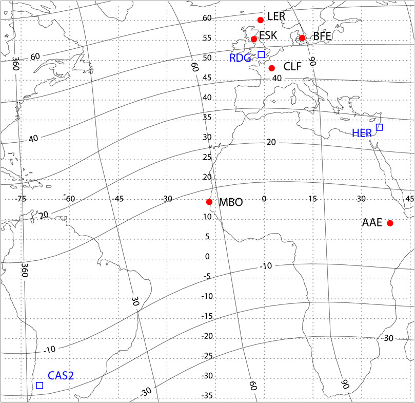
FIGURE 1. The map with location of selected atmospheric electricity stations (blue empty squares) and magnetometers (red dots). Solid lines denote geomagnetic coordinates, and dotted lines correspond to geographic coordinates.
An ideal place for monitoring the fine characteristics of atmospheric electricity is the Antarctic plateau, because of the lack of anthropogenic influences, weak and stable winds, and lack of low-altitude clouds. A large database of 10 sec atmospheric Ez and Jz observations with high-sensitive field-mill and current collector has been collected at South Pole, Vostok, and Concordia stations (Byrne et al., 1991; Few et al., 1992; Burns at al., 1998). With the use of these data, relationships between variations of the atmospheric electricity and IMF parameters (Frank-Kamenetsky et al., 1999), and the ionospheric electric potential (Corney et al., 2003) were found. The Antarctic atmospheric electricity data are available via website (http://globalcircuit.phys.uh.edu). From available 10 sec magnetometer data from South Pole observatory and atmospheric electric field and current measurements during the period 1991–1993, we have analyzed 18 SSC events.
The balloon experimenters have stored their data and made them available online (https://uh.edu/research/spg/data.html). Payloads at an altitude of ∼32 km carried 3-axis double probe electric field detectors and provided 15-s averaged 3-axis electric field data. We have re-analyzed the results of the 1985–86 Balloon Campaign at South Pole Station (Bering et al., 1987; Bering et al., 1995).
Among a large variety of MHD disturbances in the near-earth environment, special attention has been paid to the study of SSC’s caused by interaction of an interplanetary shock with the magnetosphere (Araki, 1977). The impulsive impact of a shock can bring a significant amount of energy and momentum into the magnetosphere in a very short time (Curto et al., 2007). Despite the seeming simplicity of such impact, the complexity of geomagnetic and plasma phenomena stimulated by an interplanetary shock turns out to be surprisingly large (Pilipenko et al., 2018). SSC transmission from high to low latitudes was often associated with the electric mode in the ionosphere–ground waveguide, instantly propagating along the earth’s surface (Kikuchi and Araki, 1979). Among possible electric modes in the atmospheric waveguide, the fundamental TH0 mode without a cutoff frequency is excited most effectively by a magnetospheric Alfven wave. Distinctive features of TH0 mode are the propagation velocity just somewhat less than the light speed, and weak attenuation, which is due to the geometrical factor, not due to dissipation in the ionosphere (Kikuchi, 2014). Therefore, it seems that the TH0 mode may contribute to geomagnetic response far from the MHD disturbance incident on the ionosphere (Kikuchi and Hashimoto, 2016). This notion about the TH0 mode has been applied to interpret prompt SSC transmission from auroral to low latitudes (Kikuchi, 1986; Chi et al., 2001).
However, in the original papers on the THo mode, the excitation rate of this mode by magnetospheric sources was not considered. Simple scaling shows that a vertical current Jz penetrating into the atmosphere resulting from the magnetospheric field-aligned current
In the atmosphere with exponential height-increasing conductivity
Let us estimate the expected magnitude of the vertical electric component Ez of the TH0 mode. From the subsystem of Maxwell’s equations for the E-mode, one can obtain the relationship between the components Ez and By of a wave propagating with the horizontal wave vector
Here, the dielectric permittivity is
From the relationship (Eq. 3), it follows that a TH0 mode with magnetic component By∼1 nT in the atmosphere with σ0 = 10−13 S/m must be accompanied by a spike of atmospheric electric field Ez at the earth’s surface with amplitude ∼103 V/m. Thus, even a weak magnetic signature of the E-mode must be accompanied by a burst of Ez exceeding the atmospheric potential gradient. More rigorous treatment of the problem of magnetospheric field-aligned current interaction with the multilayered ionosphere-atmosphere-ground system will be provided in Modeling of E-Mode Excitation by Magnetospheric FAC.
We compare the above theoretical estimate with simultaneous observations of the atmospheric Ez field and geomagnetic variations (X-component). We have identified >50 events with simultaneous variations of Ez and ΔX. We examine the time intervals in the ±10 min vicinity of SSC events. The plots in Figure 2 present examples, showing vertical electric field Ez (mV/m) from available stations and magnetic field ΔX (nT) component from selected stations. The data on the solar wind dynamic pressure has too many missing values for these events and are not shown. The moment of each SSC is marked by vertical lines in Figure 2.

FIGURE 2. Four events with seemingly bursts of Ez during SSC. Upper panels show variations of the atmospheric potential gradient, Ez, and bottom panel shows magnetograms (X component) from magnetometers in the same LT sector.
In a majority of the events, no response of Ez on SSC was seen. The lack of Ez response imposes a limit on a possible amplitude of an expected electric mode—it is at least less than sensor sensitivity and background noise level. In none of >50 SSC events during 2007–2019 recorded by magnetometers and atmospheric electricity stations from the GLOCAEM array or Antarctica was a similar disturbance noticed.
However, in some events, a burst of Ez during an SSC can be seen. Figure 2 presents several promising events. Let us exclude for a moment the possibility that the geomagnetic and Ez disturbances were just mere coincidences. In any case, the amplitudes of Ez disturbance occurring simultaneously with SSC do not exceed ∼10 V/m. A similar negative result was obtained using Ez and Jz observations at the South Pole station (not shown). Therefore, SSC cannot be exciting or associated with the TH0 mode.
Basic features of electric field transmission from the ionosphere into the near-earth atmosphere in the DC approximation (when the time scale is larger than the relaxation time τ > ε0/σ0 ∼ 20 min) can be understood in a simple 1D model (Park, 1976). This model predicts that a potential difference Φ between the ionosphere and ground supports Ez varying with altitude z as follows:
Here, ΣA is the total conductance of the atmospheric column
Penetration of nonsteady field, e.g., in the ULF band, is different and seldom studied. We have elaborated a model of the electromagnetic ULF response to an incidence of oscillating magnetospheric azimuthally symmetric FAC field-aligned current onto the realistic ionosphere and atmosphere. A similar multilayer model of the ionosphere-atmosphere-ground system has been used to examine the transmission of Pc1 waves through the ionosphere to the ground (Fedorov et al., 2018). The geomagnetic field B0 at high latitudes may be assumed to be vertical. The problem is azimuthally symmetric, so a cylindrical coordinate system
The model is based on a numerical solution of the full-wave equations in the realistic ionosphere. At the ground-atmosphere interface, the impedance boundary condition is imposed
The vertical profile of atmospheric conductivity is modeled by exponential dependence
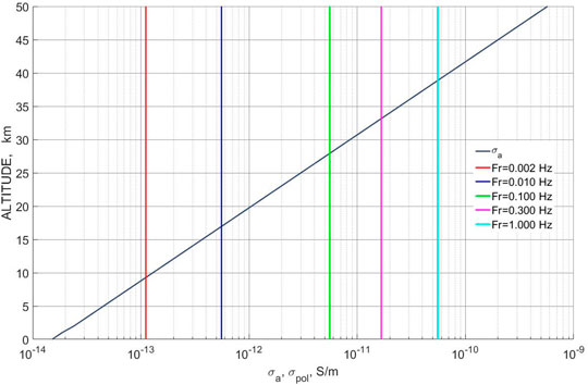
FIGURE 3. The altitude dependence of the absolute magnitude of the atmospheric conductivity |σA (z)| (black line). The magnitude of the displacement current
We have calculated both the vertical and horizontal distributions of magnetic and electric field components, including the vertical electric field in the atmosphere. The 6-component electromagnetic field is excited by an incident Alfven wave (that is, oscillatory field-aligned current) with horizontal radius R = 350 km. The amplitudes of all field components are normalized in such a way as to have the unit magnetic disturbance on the ground Bρ (z = 0) = 1 nT for all frequencies in the region of spatial maximum ρ = ρmax. The magnetic mode in the atmosphere is excited by ionospheric Hall currents. These eddy currents produce a magnetic response in the atmosphere in the radial direction, that is, in the Bρ component. The electric mode in the atmosphere is associated with vertical current. This current produces a magnetic disturbance in the azimuthal direction, that is, in the Bϕ component. Thus, Bρ and Eϕ components are associated with H-mode, while Bϕ and Eρ components are associated with the E-mode.
The radial distribution of the amplitudes of the magnetic components on the ground for various frequencies is shown in Figure 4. The maximum of Bρ (ρ) is reached at
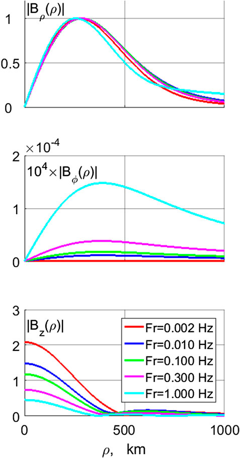
FIGURE 4. The radial distribution of the magnetic component amplitudes (in nT), from top to bottom - Bρ (ρ), Bϕ (ρ), and Bz (ρ), on the ground for various frequencies.
The radial distribution of the electric component amplitudes on the ground for various frequencies is shown in Figure 5. The electric field of the H-mode is revealed in the Eϕ component, whereas the E-mode has Eρ and Ez components. The distribution of horizontal electric components is similar to that of horizontal magnetic components (Figure 5, upper and middle panels). However, the vertical electric component Ez, associated with the E-mode, has maximum beneath the source at ρ = 0 (Figure 5, bottom panel). Amplitude of Eρ component, ∼3 10−5 mV/m, is about four orders of magnitude less than amplitude of Eϕ component, ∼0.2 mV/m. As expected for the electric field structure near the surface of a conductor, the normal to the surface electric field component Ez, ∼80 mV/m is much larger than the transverse component.
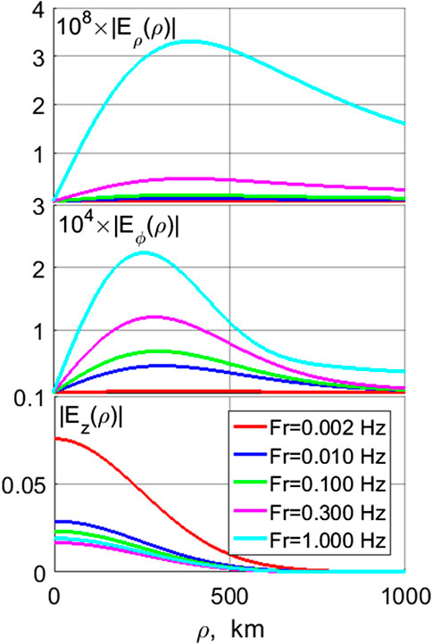
FIGURE 5. The radial distribution on the ground of the electric component amplitudes, Eρ (ρ), Eϕ (ρ), and Ez (ρ) (in V/m), for various frequencies (shown in legend).
The altitude profile of the horizontal magnetic components at the distance ρmax is presented in Figure 6. The steep variation at z∼90 km is related to a π/2 rotation of the polarization ellipse in the Е-layer. The Bρ component is nearly the same at all altitudes in the atmosphere. The Bϕ component is many orders of magnitude less than the Bρ component. The vertical magnetic component Bz is comparable in amplitude with the Bρ component and just weakly increases with altitude.
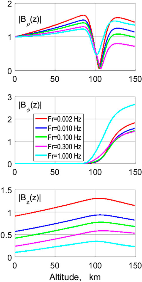
FIGURE 6. The altitudinal profiles of the horizontal magnetic components (in nT) Bρ (z), Bϕ (z) at ρ = ρmax and the vertical component
The altitude profiles of the horizontal electric field components at ρmax and vertical component Ez (z) at ρ = 0 are presented in Figure 7. The Eϕ (z) component only weakly depends on altitude for low frequencies, but for higher frequencies, it grows with altitude up to the E-layer, as expected from Faraday’s law
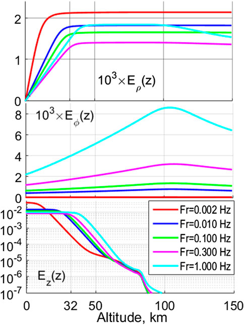
FIGURE 7. The altitudinal profiles of the horizontal electric components Eρ (z), Eϕ (z) at ρ = ρmax and the vertical component
The relative magnitude of the atmospheric electric field disturbances owing to magnetospheric ULF variations may be seen in Figure 8. This figure compares the altitude structure of all three electric field components. At the ground, the horizontal components drop to very low magnitudes prescribed by the boundary impedance relationship. On the ground, the electric field of H-mode is dominating, Eρ << Eϕ. However, because Eρ increases fast until z ∼ z*, at the balloon height (∼30 km), the electric field of the E-mode becomes much larger, Eρ >> Eϕ.
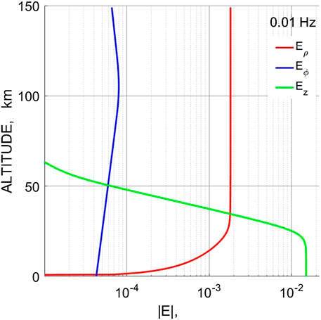
FIGURE 8. The altitudinal structure of all three electric field components Eρ (z), Eϕ (z), and Ez (z) (in V/m).
This behavior can be comprehended from the following consideration. At the earth’s surface, electric E(g) and magnetic B(g) components of the E-mode are about five orders of magnitude less than those of the H-mode. Magnetic components of both modes slowly vary with altitude: Bϕ is practically constant till ∼40 km and Bρ increases about 1.5 times only till 80 km. The behavior of electric components is more complicated. From Faraday’s law, it follows that the electric field of the H-mode varies with altitude as
Responses of the atmospheric electric field associated with impulsive and wave magnetospheric disturbances were observed during the balloon campaigns. The reported events include travelling convection vortices (TCVs) and Pc5 pulsations.
TCVs in the high latitude ionosphere are revealed on the ground as magnetic impulsive events with duration ∼5–10 min. These localized daytime disturbances are thought to be responses to transients in the solar wind or magnetosheath. A survey of the campaign data looked for unipolar magnetic pulses above background in the vertical component BZ on the ground and electric field perturbations ≥10 mV/m at balloon altitude (Lin et al., 1995). From total of 112 events found, electric field responses were observed for 90% of the events with the average Ez amplitude ∼15 mV/m.
For example, the TCV event on January 3, 1986, was recorded by both the South Pole magnetometer and the balloon electric field sensor (Bering et al., 1990). This TCV was estimated to have a radius ∼350 km and moved antisunward along the oval at a speed of ∼4 km/s. The magnetometer observed a unipolar impulse in the magnetic vertical Bz component of ∼80 nT and a bipolar impulse in the horizontal Bx component of ∼100 nT. The accompanying atmospheric electric field pulse was less than 10 mV/m in the Ez component (at the noise level), and ∼40 mV/m in the eastward Ey and ∼25 mV/m in the poleward Ex components. In another event on Jan. 14, 1986, the TCV impulse amplitudes were ∼20 nT in the horizontal magnetic and ∼15 mV/m in the electric fields. The spike in the vertical Ez field reached ∼40 mV/m.
As an example of Pc5 pulsations, the event on July 9, 1975, may be presented (Maclennan et al., 1978). During this event coincident magnetic field, transverse electric field and electron precipitation fluctuations with 5 min period were measured around ∼06 LT by ground magnetometer and balloon-borne double-probe and scintillation counter. The balloon reached a ceiling altitude of ∼35 km. The experiment recorded magnetic variations with a peak-to-peak amplitude in the Bx component of ∼6 nT and in the By component of ∼8 nT, which were coherent with horizontal electric field variations with peak-to-peak amplitudes in the N-S component Ex of ∼20 mV/m and in the E-W component Ey of ∼15 mV/m.
Thus, the normalized transverse electric field response to TCV magnetic pulses is
The expected model magnitude of an atmospheric electric field disturbance may be estimated from Figure 5 for a 1 nT magnetic disturbance. The horizontal electric field disturbance at typical balloon altitude (32 km) is about 1.5 mV/m, depending on frequency. Thus, for a typical ground magnetic amplitude (20 nT), the balloon measurements should reveal an E perturbation of about 30 mV/m. This value is in a good agreement with the results of balloon observations discussed above (e.g., Bering et al., 1990). At the same time, the inductive electric field produced by the H-mode Eϕ at balloon height would be ∼1 mV/m only.
Amplitudes of the vertical and horizontal components become comparable at an altitude of ∼30 km. For the ground magnetic disturbance with B = 1 nT and f ∼ 10 mHz, the predicted vertical electric field disturbance is ∼0.02 V/m. Thus, for intense ULF disturbances of the geomagnetic field ∼100 nT, the disturbance of the ground level atmospheric field must be ∼2 V/m. This value is small, and it can be detected by modern electric field sensors only under extremely quiet weather conditions.
Simultaneous measurements of the wave electric and magnetic components gives one the possibility to determine the apparent wave impedance in order to obtain additional information about the wave mode. This method was applied by Pilipenko et al. (2012) to the radar-measured electric field and ground geomagnetic field of Pc5 waves and by Bering et al. (1998) to the analysis of coordinated balloon-born electric and ground magnetometer measurements. More importantly, a preliminary knowledge of the atmosphere–ionosphere impedance gives one the possibility to estimate the wave electric field amplitude in the ionosphere from ground magnetometer observations.
Here, we first provide simple analytical estimates and then support them with numerical modeling. For the H-mode excited by a toroidal Alfvenic-type magnetospheric disturbance, the ratio between the dominant components of the electric field in the ionosphere, Ex, and ground magnetic response, Bx, follows from the thin ionosphere theory (Pilipenko et al., 2012):
For the E-mode, the relationship between electric field in the ionosphere and ground magnetic disturbance was derived by Hughes, (1974). Here, we present a similar relationship for a wave infinite in the E-W direction (ky = 0) and localized in N-S direction (
This ratio is altitude-dependent and does not depend on the ionospheric conductivity. At altitudes
Liu and Berkey, (1994) and Yizengaw et al. (2018) used the relationship between ionospheric electric field and magnetic field fluctuations from Hughes, (1974) to estimate the amplitude of the ionospheric electric field fluctuations driven by geomagnetic pulsations. However, the relationships they have used were incorrect choices. Moreover, it is wrong to model ULF pulsations as an E-mode.
The numerically calculated apparent impedances for both electric (E) and magnetic (H) modes (that is, the ratio E (z = 120 km)/B (z = 0) is shown in Figure 9. For the H-mode, the ratio Eρ/Bρ ∼ 0.6 (mV/m)/nT. This value is very close to the theoretical estimate (4) for ΣH∼1.4 S. For the E-mode, the ratio Eρ/Bϕ is frequency dependent, slowly decreasing from ∼102 (V/m)/nT at f ∼ 3 mHz to ∼10 (V/m)/nT at f ∼ 1 Hz. Therefore, the E-mode impedance is at least four to five orders of magnitude larger that the impedance of the H-mode. Interpretation of ULF waves as E-mode would provide unrealistically high magnitudes of the wave electric field in the ionosphere.
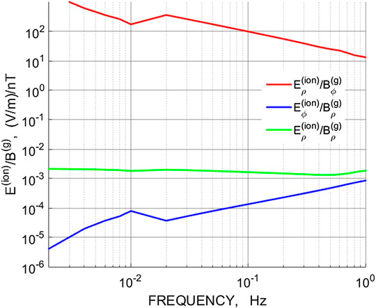
FIGURE 9. The frequency dependence of the apparent impedances (that is E (f)/B (f) amplitude ratios) for magnetic and electric modes.
An attempt to compare Pc1-3 pulsations using the South Pole search-coil magnetometer and balloon E-field data was made by Bering et al. (1998). While magnetic component was clearly observed as narrow-band emissions with power spectral densities (PSDs)
The conclusion in Estimate of EzPerturbations Accompanying Storm Sudden Commencement Events about the occurrence of large Ez in the ULF electric mode was made earlier in Zybin et al. (1974) from other considerations. The ULF field in the atmosphere can be locally approximated as an inhomogeneous plane wave with a horizontal wave vector k. In this approximation, the vertical component Ez in the field of Pc3-5 pulsations must appear. The expected magnitude of Ez must be coupled with magnetic component magnitude as follows:
Our search for an Ez signature in disturbances from magnetospheric sources has given negative results. Even for the most promising source—large-scale intense SSC impulses, observations show that the excitation of the E-mode is negligible. Therefore, the assumption of the directional analysis (Chetaev et al., 1975; Chetaev et al., 1977; Chetaev, 1985) on the occurrence of the E-mode in the incident ULF wave field is not supported by observations. Nonetheless, the mathematical formalism developed in the frameworks of the directional analysis may be applied for MTS in the ELF band (e.g., Schumann resonance).
Our numerical modeling has resulted in a rather paradoxical conclusion. Excitation of the E-mode by magnetospheric sources is very weak, and this mode practically does not contribute into the ULF wave magnetic field. The E-mode contribution into the horizontal telluric field produced by ULF pulsations is also negligible. However, in the atmosphere, at the balloon heights, the electric field of this mode becomes dominant. Thus, an adequate interpretation of coordinated balloon-ground observations of Pc5 waves and TCVs is possible only with account of multimode structure of ULF disturbance in the atmosphere comprising both H- and E-modes. The important aspect of this problem is the polarization structure of H- and E-modes (Nenovski, 1999). The pertinent theoretical modeling and comparison with data from coordinated balloon-ground observations will be considered elsewhere.
At the same time, periodic fluctuations of the atmospheric electric field Ez in the ULF range that are not associated with geomagnetic disturbances are quite common. These fluctuations may confuse and mislead a researcher upon a search of simultaneous geomagnetic and atmospheric electricity pulsations. Periodic fluctuations of the atmospheric potential gradient and vertical atmospheric current Jz in the range of Pc4-5 frequencies were observed by Yerg and Johnson, (1974) and in the Pc1 and Pc3 bands by Anisimov et al. (1984). These fluctuations were not coherent with geomagnetic pulsations, so authors suggested that they may be caused by nonmagnetospheric sources, e.g., infrasound emissions from distant meteorological sources. Pc5 pulsations of atmospheric electric field were observed near local midnight under very clear weather by balloon campaign (altitude ∼32 km) (Liao et al., 1994). Both transverse and vertical electric field components of pulsations had amplitudes of 20–30 mV/m, but no similar signal was observed in magnetometer or riometer data. Narrow-band wave packets in the Pc1 band in both horizontal and vertical components of the atmospheric electric field without a ground magnetic response were detected during the 1985–86 South Pole Balloon Campaign (Bering and Benbrook, 1995). The driving mechanisms of such “electrostatic” ULF pulsations are very speculative and have not been established.
The model implicitly assumes that a single cylindrical FAC is spread along the ionosphere out to infinity. In realistic magnetosphere–ionosphere disturbances, coupled incident and return FACs of opposite polarity are formed at various distances from each other, from about ten thousand km in SSC events to few hundred km in TCV or Pc5 events. If the geometry of the magnetosphere–ionosphere current system is known, the modeled electromagnetic fields due to each isolated FAC are to be summed up.
We have considered a simple geometry with the plane ionosphere and ground and vertical geomagnetic field B0. This assumption is well justified for the consideration of local structure of electromagnetic disturbance at distances less than 103 km from an incident FAC. At larger distances upon propagation to low latitudes, additional factors become noticeable: ionosphere/ground curvature, inclination of geomagnetic field, and lateral inhomogeneity of ionospheric parameters. However, the magnetic field decreases with distance as ∼r−2, so at large distances, the response would be too weak to observe. Probably, there is no need to advance theory to interpret very weak signatures at large distances from a source.
We have addressed the long-standing problem of coupling between atmospheric electricity and space weather disturbances at ULF time scales (from fractions minutes to tens of mins). The generation of ULF impulses and noises by atmospheric electric discharges is a more or less well-known aspect of the problem (see Pilipenko, 2012). The inverse aspect, the influence of magnetospheric magnetic disturbances on the atmospheric electric field is much less studied.
The GloCAEM atmospheric electricity field-mill measurements with 1 sec cadence have been used to examine the influence of geomagnetic SSC disturbances on atmospheric electricity. The predicted mechanism of SSC transmission by the electric-type TH0 mode along the earth–ionosphere waveguide was not confirmed. Observations with field-mills and current collectors in Antarctica also have not found any signature of the E-mode accompanying SSC magnetic pulses. Therefore, the model of prompt transmission of disturbances from auroral latitudes to low latitudes by the atmospheric TH0 mode is not supported by observations and should be rejected.
We have advanced the theory of ULF disturbance transmission though the ionosphere and atmosphere to the ground by considering the possible role of the electric mode. The constructed model of electromagnetic ULF response to an incidence of oscillating magnetospheric field-aligned current onto the realistic ionosphere is based on a numerical solution of the full-wave equations in the atmospheric-ionospheric collisional plasma whose parameters were reconstructed using the IRI model and a realistic vertical profile of atmospheric conductivity. The modeling strictly proved that excitation of the electric mode is weak and its contribution into the field of ULF waves on the ground is very small. In a most favorable situation, only a weak Ez disturbance with a magnitude of ∼several V/m could be produced by a large-scale intense (∼100 nT) geomagnetic disturbance. At the same time, the predicted amplitudes of electric field at balloon heights, ∼few tens of mV/m, induced by Pc5 pulsations and travelling convection vortices are in good agreement with coordinated balloon—ground magnetometer observations. Therefore, E-mode excitation by magnetospheric ULF disturbances cannot be completely ignored, because an adequate interpretation of balloon observations is possible only on the basis of a model comprising both H- and E-modes.
The datasets presented in this study can be found in online repositories. The names of the repository/repositories and accession number(s) can be found below: http://www.wdcb.ru/arctic_antarctic/antarctic_magn_3.ru.html.
VP performed theoretical analysis, EF did numerical modeling, VM-B analyzed data, and EB provided observational data.
This study was supported by the grants PLR-1744828 (VP) from the U.S. National Science Foundation and 20-05-00787 (EF, VM-B) from the Russian Fund for Basic Research. Details of the GloCAEM project are here https://drive.google.com/open?id=1l7VI98q4FfX5AoOEi5Y_kr-HL-58jp9E.
The authors declare that the research was conducted in the absence of any commercial or financial relationships that could be construed as a potential conflict of interest.
Alperovich, L. S., and Fedorov, E. N. (2007). “Hydromagnetic waves in the magnetosphere and the ionosphere,”in Astrophysics and space science library (Berlin, Germany: Springer Science & Business Media), Vol. 353, 418.
Anisimov, S. V., Rusakov, N. N., and Troitskaya, V. A. (1984). Short-period variations of the vertical electric current in the air. J. Geomagn. Geoelectr. 36, 229–238. doi:10.5636/jgg.36.229
Anisimov, S. V., Kurneva, N. A., and Pilipenko, V. A. (1993). Input of electric mode into the field of Pc3-4 pulsations. Geomagn. Aeron. 33 (3), 35–41.
Araki, T. (1977). Global structure of geomagnetic sudden commencements, Planet. Space Sci. 25, 373–384. doi:10.1016/0032-0633(77)90053-8
Berdichevsky, M. N., Van’jan, L. L., and Dmitriev, V. I. (1971). Concerning the possibility to neglect vertical currents during magnetotelluric sounding. Izv. AN SSSR, Fizika Zemli, N5, 69–78.
Bering, E. A., and Benbrook, J. R. (1995). Intense 2.3‐Hz electric field pulsations in the stratosphere at high auroral latitude. J. Geophys. Res. Space Phys. 100, 7791–7806. doi:10.1029/94JA02680
Bering, E. A., Benbrook, J. R., Howard, J. M., Oró, D. M., Stansbery, E. G., Theall, J. R., et al. (1987). The 1985-86 South Pole balloon campaign. Memoirs of the National Institute of Polar Research 48, 313–317.
Bering, E. A., Benbrook, J. R., Byrne, G. J., Liao, B., Theall, J. R., Lanzerotti, L. J., et al. (1988). Impulsive electric and magnetic field perturbations observed over South Pole: flux transfer events? Geophys. Res. Lett. 15, 1545–1548. doi:10.1029/GL015i013p01545
Bering, E. A., Lanzerotti, L. J., Benbrook, J. R., Lin, Z.‐M., Maclennan, C. G., Wolfe, A., et al. (1990). Solar wind properties observed during high-latitude impulsive perturbation events. Geophys. Res. Lett. 17, 579–582. doi:10.1029/GL017i005p00579
Bering, E. A., Benbrook, J. R., Liao, B., Theall, J. R., Lanzerotti, L. J., and MacLennan, C. G. (1995). Balloon measurements above the South pole: study of the ionospheric transmission of ULF waves. J. Geophys. Res. 100, 7807–7820. doi:10.1029/94JA02810
Bering, E. A., Benbrook, J. R., Engebretson, M. J., and Arnoldy, R. L. (1998). Simultaneous electric and magnetic field observations of Pc1–2 and Pc3 pulsations. J. Geophys. Res.: Space Physics 103, 6741–6761. doi:10.1029/97JA03327
Burns, G. B., Frank-Kamenetsky, A. V., Troshichev, O. A., Bering, E. A., and Papitashvili, V. O. (1998). The geoelectric field: a link between the troposphere and the ionosphere. Ann. Glaciol. 27, 651–654. doi:10.3189/1998AoG27-1-651-654
Byrne, G. J., Bering, E. A., Few, A. A., and Morris, G. A. (1991). Measurements of atmospheric conduction currents and electric fields at the South pole. Antarct. J. U. S. 26, 291–294.
Chetaev, D. N. (1970). About structure of geomagnetic pulsation field and magnetotelluric soundings. Solid Earth Phy. 2, 52–56.
Chetaev, D. N. (1985). Directional analysis of magnetotelluric observations. Moscow: Nauka, 228.[in Russian]
Chetaev, D. N., Fedorov, E. N., Krylov, S. M., Lependin, V. P., Morghounov, V. A., Troitskaya, V. A., et al. (1975). On the vertical electric component of the geomagnetic pulsation field. Planet. Space Sci. 23, 311–314. doi:10.1016/0032-0633(75)90136-1
Chetaev, D. N., Chernysheva, S. P., Morghounov, V. A., Sheftel, V. A., and Zemliankin, G. A. (1977). On the pulsations of Ez(air) in the frequency range of Pc1. Planet. Space Sci 26, 507–508. doi:10.1016/0032-0633(78)90071-5
Chi, P. J., Russell, C. T., Raeder, J., Zesta, E., Yumoto, K., Kawano, H., et al. (2001). Propagation of the preliminary reverse impulse of sudden commencements to low latitudes. J. Geophys. Res. 106, 18857–18864. doi:10.1029/2001JA900071
Corney, R. G., Burns, G. B., Michael, K., Frank-Kamenetsky, A. V., Troshichev, O. A., Bering, E. A., et al. (2003). The influence of polar-cap convection on the geoelectric field at Vostok, Antarctica. J. Atmos. Sol. Terr. Phys. 65, 345–354. doi:10.1016/S1364-6826(02)00225-0
Curto, J. J., Araki, T., and Alberca, L. F. (2007). Evolution of the concept of Sudden storm commencements and their operative identification. Earth Planets Space 59, i–xii. doi:10.1186/BF03352059
Dmitriev, V. I. (1970). Impedance of a stratified media for an inhomogeneous plane wave. Izv. AN SSSR. Fizika Zemli N7, 63–69.
Fedorov, E. N., Pilipenko, V. A., Engebretson, M. J., and Hartinger, M. D. (2018). Transmission of a magnetospheric Pc1 wave beam through the ionosphere to the ground. J. Geophys. Res. B: Space Phys. 123, 3965–3982. doi:10.1029/2018JA0253381–18
Few, A. A., Morris, G. A., Bering, E. A., Benbrook, J. R., Chadwick, R., and Byrne, G. J. (1992). Surface observations of global atmospheric electric phenomena at Amundsen-Scott South Pole Station. Antarct. J. U. S. 27, 307–309.
Frank-Kamenetsky, A. V., Burns, G. B., Troshichev, O. A., Papitashvili, V. O., Bering, E. A., and French, W. J. R. (1999). The geoelectric field at Vostok, Antarctica: it’s relation to the interplanetary magnetic field and the polar cap potential difference. J. Atmos. Sol. Terr. Phys. 61, 1347–1356. doi:10.1016/S1364-6826(99)00089-9
Hameiri, E., and Kivelson, M. G. (1991). Magnetospheric waves and the atmosphere-ionosphere layer. J. Geophys. Res. 96, 21125–21134.
Harrison, R. G., Aplin, K. L., and Rycroft, M. J. (2010). Atmospheric electricity coupling between earthquake regions and the ionosphere. J. Atmos. Sol. Terr. Phys. 72, 376–381. doi:10.1016/j.jastp.2009.12.004
Hughes, W. J., and Southwood, D. J. (1976). The screening of micropulsation signals by the atmosphere and ionosphere. J. Geophys. Res. 81, 3234–3240. doi:10.1029/JA081i019p03234
Hughes, W. J. (1974). The effect of the atmosphere and ionosphere on long period magnetospheric micropulsations. Planet. Space Sci 22, 1157–1172. doi:10.1016/0032-0633(74)90001-4
Kikuchi, T. (1986). Evidence of transmission of polar electric field to the low latitude at times of geomagnetic sudden commencement. J. Geophys. Res. 91, 3101–3105. doi:10.1029/JA091iA03p03101
Kikuchi, T. (2014). Transmission line model for the near-instantaneous transmission of the ionospheric electric field and currents to the equator. J. Geophys. Res. 119, 1131–1156. doi:10.1002/2013JA019515
Kikuchi, T., and Araki, T. (1979). Transient response of uniform ionosphere and preliminary reverse impulse of geomagnetic storm sudden commencement. J. Atmos. Terr. Phys. 41, 917–925. doi:10.1016/0021-9169(79)90093-X
Kikuchi, T., and Hashimoto, K. K. (2016). Transmission of the electric fields to the low latitude ionosphere in the magnetosphere-ionosphere current circuit. Geoscience Letters 3, 1–11. doi:10.1186/s40562-016-0035-6
Kleimenova, N. G., Nikiforova, N. N., Kozyreva, O. V., and Michnowsky, S. (1996). Long-period geomagnetic pulsations and fluctuations of the atmospheric electric field intensity at the polar cap latitudes. Geomagn. Aeron. 35 (N4), 469–477.
Kokorowski, M., Sample, J. G., Holzworth, R. H., Bering, E. A., Bale, S. D., Blake, J. B., et al. (2006). Rapid fluctuations of stratospheric electric field following a solar energetic particle event. Geophys. Res. Lett. 33, L20105. doi:10.1029/2006GL027718
Liao, B., Benbrook, J. R., Bering, E. A., Byrne, G. J., Theall, J. R., Lanzerotti, L. J., et al. (1994). Balloon observations of nightside Pc5 quasi‐electrostatic waves above the South Pole. J. Geophys. Res.: Space Physics 99, 3879–3891. doi:10.1029/93JA02753
Lin, Z. M., Bering, E. A., Benbrook, J. R., Liao, B., Lanzerotti, L. J., Maclennan, C. G., et al. (1995). Statistical studies of impulsive events at high latitudes. J. Geophys. Res.: Space Physics 100, 7553–7566. doi:10.1029/94JA01655
Liu, J. Y., and Berkey, F. T. (1994). Phase relationships between total electron content variations, Doppler velocity oscillations and geomagnetic pulsations. J. Geophys. Res. 99, 17539–17545. doi:10.1029/94JA00869
Maclennan, C. G., Lanzerotti, L. J., Hasegawa, A., Bering, E. A., Benbrook, J. R., Sheldon, W. R., et al. (1978). On the relationship of ∼3 mHz (Pc5) electric, magnetic, and particle variations. Geophys. Res. Lett. 5, 403–406. doi:10.1029/GL005i005p00403
Nenovski, P. (1999). Asymmetry in the electric and magnetic field polarization of geomagnetic pulsations. J. Atmos. Sol. Terr. Phys. 61, 1007–1015. doi:10.1016/S1364-6826(99)00048-6
Nicoll, K. A., Harrison, R. G., Barta, V., Bor, J., Brugge, R., et al. (2019). Towards a global network for atmospheric electric field monitoring. J. Atmos. Sol. Terr. Phys. 184, 18–29. doi:10.1016/j.jastp.2019.01.003
Park, C. G. (1976). Downward mapping of high-latitude ionospheric electric fields to the ground. J. Geophys. Res. 81, 168–174. doi:10.1029/JA081i001p00168
Pilipenko, V. A. (2012). Impulsive coupling between the atmosphere and ionosphere/magnetosphere. Space Sci. Rev. 168, 533–550. doi:10.1007/s11214-011-9859-8
Pilipenko, V., Vellante, M., Anisimov, S., De Lauretis, M., Fedorov, E., and Villante, U. (1998). Multi-component ground-based observation of ULF waves: goals and methods. Ann. Geofisc. 41, 63–77. doi:10.4401/ag-3794
Pilipenko, V., Belakhovsky, V., Kozlovsky, A., Fedorov, E., and Kauristie, K. (2012). Determination of the wave mode contribution into the ULF pulsations from combined radar and magnetometer data: method of apparent impedance. J. Atmos. Sol. Terr. Phys. 77, 85–95. doi:10.1016/j.jastp.2011.11.013
Pilipenko, V. A., Bravo, M., Romanova, N. V., Kozyreva, O. V., Samsonov, S. N., and Sakharov, Y. A. (2018). Geomagnetic and ionospheric responses to the interplanetary shock wave of March 17, 2015. Izvestiya Phys. Solid Earth 54 (N5), 721–740. doi:10.1134/S1069351318050129
Savin, M. G., Nikiforov, V. M., and Kharakhinov, V. M. (1991). About anomalies of vertical electric component of telluric field at Northern Sakhalin. Izv. AN SSSR. Fizika Zemli N2, 100–108.
Vinogradov, I. A. (1960). New experimental data on vertical component of short-period oscillations of telluric current field. Geol. and Geophys. В6, 100–105.
Yerg, D. G., and Johnson, K. R. (1974). Short‐period fluctuations in the fair‐weather electric field. J. Geophys. Res. 79, 2177–2184. doi:10.1029/JC079i015p02177
Yizengaw, E., Zesta, E., Moldwin, M. B., Magoun, M., Tripathi, N. K., Surussavadee, C., et al. (2018). ULF wave‐associated density irregularities and scintillation at the equator. Geophys. Res. Lett. 45, 5290–5298. doi:10.1029/2018GL078163
Yumoto, K., Pilipenko, V., Fedorov, E., Kurneva, N., and De Lauretis, M. (1997). Magnetospheric ULF wave phenomena stimulated by SSC. J. Geomagn. Geoelectr. 49, 1179–1195. doi:10.5636/jgg.49.1179
Keywords: atmosphere, ionosphere, ultra-low-frequency waves, magnetic and electric modes, balloon observations, ssc
Citation: Pilipenko VA, Fedorov EN, Martines-Bedenko VA and Bering EA (2021) Electric Mode Excitation in the Atmosphere by Magnetospheric Impulses and ULF Waves. Front. Earth Sci. 8:619227. doi: 10.3389/feart.2020.619227
Received: 19 October 2020; Accepted: 09 December 2020;
Published: 27 January 2021.
Edited by:
Irina Alexandrovna Mironova, Saint Petersburg State University, RussiaReviewed by:
W. Jeffrey Hughes, Boston University, United StatesCopyright © 2021 Pilipenko, Fedorov, Martines-Bedenko and Bering.. This is an open-access article distributed under the terms of the Creative Commons Attribution License (CC BY). The use, distribution or reproduction in other forums is permitted, provided the original author(s) and the copyright owner(s) are credited and that the original publication in this journal is cited, in accordance with accepted academic practice. No use, distribution or reproduction is permitted which does not comply with these terms.
*Correspondence: V. A. Pilipenko, c3BhY2Uuc29saXRvbkBnbWFpbC5jb20=
Disclaimer: All claims expressed in this article are solely those of the authors and do not necessarily represent those of their affiliated organizations, or those of the publisher, the editors and the reviewers. Any product that may be evaluated in this article or claim that may be made by its manufacturer is not guaranteed or endorsed by the publisher.
Research integrity at Frontiers
Learn more about the work of our research integrity team to safeguard the quality of each article we publish.