10-year Characteristics of Moisture Source Regions and Their Potential Effect on Seasonal Isotopic Signatures of δ18O in Tropical Trees of Southern Ecuador

Ratios of stable oxygen isotopes in tree rings (δ¹⁸O) are a valuable proxy for reconstructing past climates. Such reconstructions allow us to gain better knowledge of climate dynamics under different (eg warmer) environmental conditions, which also forms the basis for effective risk management. The latter aspect is particularly relevant for our study site on the western flanks of the Andes in Southern Ecuador, since the region is frequently affected by droughts and heavy precipitation events during the rainy season (January to April), leading to enormous social and economic losses. In particular, we focus on precipitation amounts and moisture source regions as they are known to influence the δ¹⁸O signature of tree rings. Moisture source regions are based on 240 h backward trajectories that were calculated with the trajectory model LAGRANTO for the rainy seasons 2008 to 2017. A moisture source diagnostic was applied to the air parcel pathways. The resulting moisture source regions were analyzed by calculating composites based on precipitation amounts, season, and calendar year. The precipitation amounts were derived from data of a local Automatic Weather Station (AWS). The analysis confirms that our study site receives its moisture both, from the Atlantic and the Pacific Oceans. Heavy precipitation events are linked to higher moisture contributions from the Pacific, and local SST anomalies along the coast of Ecuador are of higher importance than those off the coast toward the central Pacific. Moreover, we identified increasing moisture contributions from the Pacific over the course of the rainy season. This change and also rain amount effects are detectable in preliminary data of δ¹⁸O variations in tree rings of Bursera graveolens. These signatures can be a starting point for investigating atmospheric and hydroclimatic processes, which trigger δ¹⁸O variations in tree rings, more extensively in future studies.

Introduction

Ecuador and in particular its share of the western flanks of the tropical Andes are prone to heavy rain events and floods that occur with a high interannual variability (Endlicher et al., 1989; Bendix, 2000; Bendix et al., 2003; Bendix and Bendix, 2006; Takahashi and Martinez, 2019). Such events often lead to high social and economic losses (Vos et al., 1999). To facilitate and enable a better risk management for the affected population, a solid knowledge about long-term precipitation dynamics is obligatory (Kieslinger et al., 2019). However, meteorological data are sparse for this region (Emck, 2008; Kieslinger et al., 2019). Reconstructions of past climate variability are a promising tool to gain further insight into natural precipitation variability and its underlying climatic drivers.

Climate reconstructions can be established by using tree rings or others archives, including marine and lacustrine sediments or ice cores are also utilized as paleoclimatic proxies (Braeuning, 2009). However, tree rings have a number of advantages. The most desirous ones are the dating accuracy on an annual basis and the high temporal resolution, up to intraseasonal (Jones et al., 2009). Moreover, multiple replication of tree-ring chronologies allows to determine uncertainty estimates. Making use of the oxygen isotopic signature instead of the annual increments of tree rings adds another benefit, because the processes controlling the incorporation of stable oxygen isotopes into plant material are well understood (McCarroll and Loader, 2004).

Oxygen isotopes in tree-ring cellulose are, to a certain degree, a record of the isotopic composition of precipitation. The isotopic composition of oxygen (δ¹⁸O) is expressed as the ratio of the heavier ¹⁸O to the lighter ¹⁶O with respect to standard mean ocean water or to the Vienna Standard Mean Ocean Water (VSMOW). However, until the isotopes are incorporated within the tree cell, fractionation processes change the initial isotopic ratio of the moisture at its source region by discriminating one stable isotope of oxygen over the other (McCarroll and Loader, 2004; van der Sleen et al., 2017). With increasing distance to the moisture source region, δ¹⁸O decreases due to Rayleigh distillation, which describes a rain out effect of the heavier ¹⁸O (Dansgaard, 1964; Gat, 1996). After the condensation of moisture, falling rain droplets are exposed to evaporation and merge with other droplets. This is known as amount effect, meaning that heavy and long-lasting precipitation events lead to lower δ¹⁸O values. This effect is especially effective in the tropics (Dansgaard, 1964). At the soil surface and at the leaf level within the plant, evaporation leads to the enrichment of heavy ¹⁸O, due to the preferred evaporation of the lighter ¹⁶O (Gat, 1996; van der Sleen et al., 2017).

Gat (1996) pointed out that the isotopic composition of precipitation reflects different moisture source regions. Recent tree-ring oxygen isotope studies were able to detect these differing isotopic signatures due to variations of δ¹⁸O in annually resolved tree rings (Grießinger et al., 2018; Meier et al., 2020). In contrast, Muangsong et al. (2020) revealed the influence of varying moisture sources on the isotopic composition solely within intra-seasonally but not within annually resolved δ¹⁸O tree-ring chronologies from the tropics.

In the tropics, stable isotope analysis of oxygen within tree rings are still sparse. Since it was recognized that some tropical tree species form annual growth rings and the understanding of stable isotopes had improved, the number of studies has increased over the past decade (van der Sleen et al., 2017). Although one tree-ring oxygen isotope study from a mountain rainforest exists in southern Ecuador (Volland et al., 2016), its representativity for the western slopes of the Andes is limited. This is attributed to the location of their study region on the eastern flanks of the Andes, which is exposed to a different climatic regime (Volland et al., 2016). By investigating tree ring widths of tree species on the western flanks of southern Ecuador, Pucha-Cofrep et al., (2015) showed that the semi-deciduous tree species Bursera graveolens is suitable for paleoclimatie reconstructions.

Climatologically, the western slopes of the Andes in southern Ecuador experience a rainy season, mainly from January to April (Bendix and Lauer, 1992; Emck, 2008; Volland-Voigt et al., 2011; Kieslinger et al., 2019). During this time, Southern Ecuador lies in between the influence of two air masses. On the one hand, northwesterly winds prevail originating in the northern hemisphere (Bendix and Lauer, 1992). On the other hand, southeasterly trade winds from the South Pacific subtropical high-pressure system approach the continent as recurved westerlies at the surface (Bendix and Lauer, 1992; Emck, 2008). Especially heavy precipitation events are associated with westerlies that transport moisture from the tropical Pacific to the western slopes of the Andes (Bendix, 2000; Emck, 2008; Volland-Voigt et al., 2011). These westerlies are a rather regional and complex phenomenon (Emck, 2008). They facilitate the development of a land-sea breeze system. These, in turn, can interact with up-slope winds, extend toward the Andes and trigger convection (Horel and Cornejogarrido, 1986; Bendix, 2000; Emck, 2008). In the mid to upper troposphere, these flows impinge on the prevailing easterly trade winds from the Amazon, which are not blocked by the Andes. This process may lead to moisture entrainment (Bendix, 2000). Another important process for the formation of precipitation is convection (Emck, 2008; Rollenbeck and Bendix, 2011). In summary, moisture sources for precipitation in the study region of interest are the eastern Pacific and the Amazon, which has also been demonstrated by backward trajectory modeling (Trachte, 2018). However, to our knowledge, no previous study has investigated the particular moisture source regions and their individual contribution to regional precipitation events. Understanding the effect of moisture sources on the isotopic composition of tree rings is necessary for hydroclimatic reconstructions in future studies.

In our study, we evaluate the influence of different precipitation events and their moisture source regions on the oxygen isotopic signature of Bursera graveolens tree rings in southwestern Ecuador during the rainy season on interannual and intra-annual time scales.

For this purpose, the two main goals are

(1) to investigate local precipitation events and

(2) to identify moisture source regions based on trajectories for different composites (precipitation events, each month and each calendar year).

To put the two goals in a wider context and future perspective, we also discuss a possible relationship between precipitation as well as moisture source regions and the isotopic signatures in Bursera graveolens tree rings.

Materials and Methods

We investigated local precipitation events using the data of an automatic weather station (AWS). To ensure a high quality of the study, we screened the local precipitation record for missing values. The identified local precipitation events were related to moisture source regions by classifying daily precipitation amounts into three categories. This also enabled the composite analysis of moisture sources. Moisture source regions are the core of our study and were computed using a backward trajectory model that is based on ERA5 reanalysis data. To have confidence in the selected reanalysis product, we evaluated it against the local AWS data and against the Modern-Era Retrospective Analysis for Research and Applications-2 (MERRA2)—another high-resolution reanalysis product. Finally, we discuss the oxygen isotopic signatures in Bursera graveolens tree rings with respect to precipitation and the identified moisture source regions.

Before describing the datasets used, we give an overview of the study site and describe, afterward, all applied laboratory and statistical methods.

Study Site

The study site (4.21471°S, 79.8854°W) in southern Ecuador is located in the “Laipuna Nature Reserve,” a strictly protected ecosystem (UNESCO, 2017) that lies between the Pacific coast and the western flanks of the Andes (Pucha-Cofrep et al., 2015). It features a seasonally dry tropical forest (Särkinen et al., 2012) in a semihumid climate ranging from 590 m above sea level up to 1,480 m above sea level in altitude (Pucha-Cofrep et al., 2015).

Temperature variations are small over the course of the year with an annual average of 23.4°C (Pucha-Cofrep et al., 2015). Precipitation occurs mostly during night time (Volland-Voigt et al., 2011) and the rainy season lasts from January to May (Pucha-Cofrep et al., 2015) or from January to April (Volland-Voigt et al., 2011). Precipitation amounts in May are usually low (Pucha-Cofrep et al., 2015), why we consider the rainy season lasting from January to April. During the dry season, precipitation is impeded due to the permanent establishment of the South Pacific subtropical high-pressure system and its related inversion. This atmospheric stability is reduced during the rainy season, which is associated with an approaching of northeast trade winds from the northern hemisphere that finally recurve to northwesterly winds (Bendix and Lauer, 1992).

The high inter-annual precipitation variability (Spannl et al., 2016) is associated with the El Niño Southern Oscillation (ENSO) phenomenon (Bendix, 2000; Bendix et al., 2003; Bendix and Bendix, 2006; Bendix et al., 2011; Vicente-Serrano et al., 2017), which describes the alternation of anomalously cold and warm sea surface temperatures (SSTs) in the tropical Pacific Ocean. The warm anomalies, known as El Niño, can be distinguished based on the location of maximum warming, into central Pacific, eastern Pacific and coastal El Niño. In contrast, La Niña is related to cold SST anomalies in the central or eastern tropical Pacific (McPhaden et al., 2006; Capotondi et al., 2015; Wang et al., 2017; Echevin et al., 2018; Takahashi and Martinez, 2019).

Data

Automatic Weather Stations

From April 2007 to March 2015, a field experiment was conducted to provide insight into the meteorological conditions at the study site. Therefore, two AWSs (THIES Climate, Germany) were employed, namely “Laipuna Valley” (590 m above sea level, 4.21471°S, 79.8854°W, Valley Station) and “Laipuna Mountain” (1,450 m above sea level, 4.23782°S, 79.8988°W, Mountain Station). Both recorded temperature (at 2 m), relative humidity (at 2 m), wind speed and direction (at 2.5 m) and precipitation (at 1 m) above the ground at 10-min intervals that were stored as hourly means (Volland-Voigt et al., 2011; Pucha-Cofrep et al., 2015; Spannl et al., 2016).

We based this study on the data of the Valley Station, since it features a lower number of missing values (see Time Aggregates and Missing Values) resulting in a higher robustness of our computations. However, for the evaluation of the reanalysis dataset, we also used the data of the Mountain Station to capture the whole range of climate variability in the study region.

Reanalysis Products

ERA5 is the latest reanalysis product from the European Center for Medium-Range Weather Forecasts (ECMWF) (C3S, 2017). Currently, the data can be obtained from 1979 onward and are provided as instantaneous values. In comparison to its forerunner, ERA-Interim (Dee et al., 2011), major improvements were achieved in the overall data quality. Among others, this can be attributed to its high spatial resolution of 31 km in the horizontal and 137 levels to 1 hPa in the vertical, an improved 12-h 4D-Var assimilation technique and an advanced sea surface temperature dataset. Moreover, the number of assimilated observations was increased, resulting in about 24 million observations per day at the end of 2018, which is almost five times greater than for ERA-Interim. Beside the overall rising availability of observations, the capability of handling other data formats contributed to this advance (Hersbach et al., 2018; Hersbach et al., 2019).

MERRA2 is generated by the NASA’s Global Modeling and Assimilation Office (GMAO) and is their latest version of atmospheric reanalysis covering the modern satellite era from 1980 to 2020. By applying the Goddard Earth Observing System-5 (GEOS-5), the output data can be retrieved with a spatial resolution of 0.625° × 0.5° in longitude and latitude at hourly timesteps (Gelaro et al., 2017). For MERRA2, we choose the hourly product that is time averaged, since the AWS data features the same characteristic.

Tree Ring δ¹⁸O Isotopes

Bursera graveolens is a tropical tree species that develops distinct annual growth boundaries and was proven to be suitable for tree ring width studies (Rodríguez et al., 2005; Pucha-Cofrep et al., 2015). In March 2018, we collected 10 core samples of Bursera graveolens located in the vicinity of the Valley Station. The distance from the AWS was restricted to a maximum of 50 m. Three cores (A, B, C) allowed a distinction of annual increments. The cores were separated with a sledge microtome into 80 µm thin slices to capture also the intraannual variability. The oxygen isotope ratio (¹⁸O/¹⁶O, expressed as δ¹⁸O) of the wholewood slices were analyzed using an isotope ratio mass spectrometer (Delta V Advantage, Thermo Finnigan) coupled to an OPTIMA elemental analyzer. Therefore, each slice was pyrolyzed to CO at 1,080°C. The measured ratio (RSample) is finally expressed as deviation from the Vienna Standard Mean Ocean Water (VSMOW, RStandard) with δ¹⁸O = (RSample/RStandard − 1) × 1,000. The resulting error (analytical) comes to ±0.3‰. The lack of enough wood material did not allow us to extract and determine the more precise δ¹⁸O ratios of tree ring alpha cellulose. A total number of 810 (A = 259, B = 238, C = 310) isotope samples were analyzed. An accurate annual dating of the intra-annual tree ring isotope values was only possible for two cores (A, B), resulting in 497 data points suitable for the discussion. These two time series cover the years from 2012 to 2017.

Methods

Time Aggregates and Missing Values

Precipitation is the variable of main interest in this study. All other variables (wind, temperature and relative humidity) were just utilized to validate the reanalysis dataset. Hence, a differentiated consideration of its calculation and the handling of its missing values is appropriate.

The daily values of wind, temperature and relative humidity were calculated as means from hourly values. Hereby, only daily means were considered, where all 24 values were existing, otherwise, it was flagged as missing. In this way, we ensured that the quality is as good as possible. In most of the concerned cases, all values of a day were missing.

Precipitation was considered on a daily, monthly, rainy season and an annual basis. As before, daily values were only calculated as sums when all 24 values were available. For the monthly, rainy season and annual sums, this approach would have led to too many missing values. Therefore, we calculated monthly mean values as average of daily sums multiplied by the number of days of a month. The rainy season and the annual values are the sums of all respective monthly values.

The percentage of missing values in the AWS data for all variables at hourly and daily resolution during the rainy season lies between 3.6% and 12.5% for the Valley Station (Table 1), whereas it is 18.8%–34.4% for the Mountain Station. This difference makes the Valley Station to the more appropriate dataset for our study.

TABLE 1

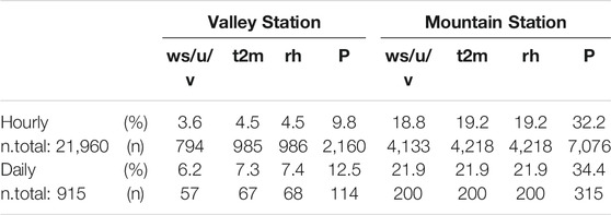
TABLE 1. Percentage and total number (n.total) of missing values of the Valley and Mountain Station for daily and hourly values during the rainy season encompassing all variables considered in the evaluation of the AWS data.

Precipitation, in comparison to the other variables, has the highest amount of missing values. This can be attributed to known issues with precipitation measurements (e.g., leaves or insects clogging the rain collector). In particular, missing values at the Valley Station amount to 9.8% and 12.5%, for hourly and daily sums, respectively (Table 2). The strict approach of just calculating daily sums, when all values of a day are existent, led to an increase of 1% (not shown). For daily sums, which are of main importance in this study, the total number of missing days is 114 days out of 915 days. These days were neglected in the composite analysis of moisture source regions regarding precipitation events and just reduced the number of available cases. The monthly percentage of missing values is 6.5% whereas the rainy season one is 11.1%.

TABLE 2

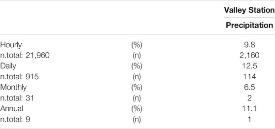
TABLE 2. Percentage and total number (n.total) of missing values of the Valley Station for hourly, daily, monthly and annual/rainy season precipitation sums.

Evaluation of ERA5 Reanalysis Dataset

Our evaluation was subdivided into two parts. In the first, we showed that ERA5 is a suitable reanalysis product for our study region and appropriate as input dataset for the trajectory model. Therefore, we compared statistical measures of all available AWS variables against the ones from both reanalysis datasets. In the second part, we focused on precipitation variability to see whether total precipitation is representative in ERA5.

For both analyses, it needs to be kept in mind, that we cannot expect a perfect quantitative fit, due to the present scale mismatch between the AWS point measurements and the gridded reanalysis products that consist of area mean values (Tustison et al., 2001; Moelg and Kaser, 2011). The evaluation rather aimed to explore whether the reanalysis product is a realistic regional framework.

Evaluation of ERA5 Reanalysis Against MERRA2 and Both Automatic Weather Stations

The evaluation of ERA5 for all available AWS variables considered wind speed and direction, temperature, precipitation and relative humidity. Hereby, we compared the ERA5 reanalysis datasets against MERRA2 and both AWSs (Mountain Station and Valley Station). For the reanalysis data, we obtained hourly values covering the same time period as the AWS data. In particular, we used u- and v-winds and calculated the respective wind speeds. To ease the evaluation of the wind direction, we made use of the u-und v-components. Therefore, we extracted the u- and v-wind velocities from the AWS wind direction. Moreover, we retrieved from both reanalysis datasets total precipitation, 2-m temperature and dew-point temperature. The latter two were utilized to calculate relative humidity (Alduchov and Eskridge, 1996). For ERA5, as well as for MERRA2, we picked the two grid points that were closest to our study site, since a single closest grid point could not be clearly identified. In this study, we permanently refer to the mean between both grid cells. We conducted the evaluation for the rainy season on an hourly and daily basis. Boxplots were generated to capture the median and inter-quartile range, whereas the whiskers showed the whole range of all values. Moreover, we considered statistical measures like the mean bias, root mean square error (rmse) and the correlation coefficient (corrcoef). For precipitation, we calculated the Spearman correlation coefficient, whereas for all other variables we determined the Pearson correlation coefficient. The correlation was defined as significant with a p-value < 0.001.

Evaluation of ERA5 Precipitation Variability

The evaluation of total precipitation from ERA5 was conducted by comparing the daily and the seasonal cycles and the interannual variability against those of the AWS. Here and onwards, we only considered the Valley Station as reference dataset, due to the lower number of missing values. As before, the analysis was restricted to the rainy seasons from April 2007 until March 2015. The mean daily cycle was calculated as mean of the respective hour from all rainy season hourly values. For the seasonal cycle, monthly precipitation sums were calculated and averaged for each calendar month. For completeness, the monthly values of the dry season are also shown. The same applies to the annual sums that also incorporate values of the dry season. Annual and rainy season sums of ERA5 are additionally provided for the years 2015–2017.

Analysis of Precipitation Events

To better understand precipitation characteristics, we investigated the duration and occurrence of local events. Therefore, we considered the time series and the distribution of daily sums of precipitation during the rainy season calculated from the available data of the Valley Station from 2008 to 2015. A histogram was utilized to assign days into three classes. The first class “no rain” (total number of days: 254) encompasses all days without any rain (p = 0 mm). Days with precipitation sums between 1 and 5 mm belong to “normal rain” (total number of days: 119) days, which refers to all values between the 60th and 80th percentile. Daily precipitation sums between the 40th and the 60th percentile, which would have been the desirable percentile range for the “normal rain” day, cover precipitation values between 0.1–1 mm, which is too close to the “no rain” class. Consequently, we decided to choose higher percentiles. “Heavy rain” (total number of days: 77) days with p > 12 mm/day describe all days above the 90th percentile. Not all days were considered in this classification scheme, which allowed to recognize differences between the characteristics of typical events more clearly (Moelg et al., 2009).

Moisture Sources Based on Backward Trajectories

Trajectories were used to determine moisture source regions. However, we were not only interested in the region, but in the contribution of each moisture source region to the precipitation at the study site. For this moisture source diagnostic, we followed the approach of Sodemann et al. (2008).

Trajectories and Their Moisture Content

Backward trajectories, which describe the movement of an air parcel in space and back in time, were utilized in different studies to identify moisture sources (Sodemann et al., 2008; Soderberg et al., 2013; Grießinger et al., 2018; Jana et al., 2018; Langhamer et al., 2018; Trachte, 2018).

In our study, we carried out the trajectory analysis using LAGRANTO (Sprenger and Wernli, 2015) driven by ERA5 input data. The model is based on a Lagrangian approach using wind and surface pressure fields to calculate trajectories of air parcels (Wernli and Davies, 1997). It lifted air parcels by 10 hPa when they would have crossed the surface and hence the model’s lower boundary. In our study, the starting points, where the backward calculations begin (t = 0), were horizontally equidistantly distributed with a distance of 5 km within a circle (∅20 km) around the location of the observational site (4.21471° S, 79.8854° W), which results in 51 starting points at one pressure level. In the vertical, we chose eight pressure levels that have an equidistance of 50 hPa between 850 hPa and 500 hPa. Trajectories were calculated 240 hours back in time, starting four times a day at 5 a.m., 11 a.m., 5 p.m. and 11 p.m. UTC to capture the daily cycle. This was done for the rainy seasons covering the available data (AWS 2008–2015; oxygen isotopes 2012–2017) from 16 January to 30 April from 2008 to 2017 (1,050 days). In total, 1,713,600 (51 × 8 × 4 × 1,050) trajectories were calculated. We set the temporal resolution of the trajectories to 1 hour resembling the ERA5 input dataset. The study site is located within complex topography. This circumstance makes the calculation of trajectories challenging and could lead to spatial deviations (Stohl et al., 1995). The trajectory error is growing with increasing backward time. This error becomes significant after a backward calculation time of ten days (Stohl et al., 1995; Stohl and Seibert, 1998; Sodemann et al., 2008). As we do not surpass these ten days of backward calculation time, we are confident in our trajectory calculations.

As basis for the moisture source analysis, specific humidity (q) was traced along each trajectory. Changes in the moisture content of an air parcel (Δq) are mainly based on evaporation (E) and precipitation (P). The sign of Δq determines the dominating process during a time step:

$\Delta q=E-P$

At one time step, only the dominating moisture process is considered, so either moisture uptake or loss. This effect is reduced with the high temporal resolution of 1 hour of ERA5 in comparison to studies using coarser ones. Other processes, like mixing with nearby air parcels or the existence of ice and liquid water particles are neglected (Sodemann et al., 2008).

Selection of Trajectories

For our study, we are only interested in trajectories that contribute to precipitation at the study site. Therefore, we undertook a selection procedure, where the following requirements had to be fulfilled (Sodemann et al., 2008):

(1) Δq at the starting point [Δq₀ (t = 0)] had to be negative with respect to the former time step

(2) Relative humidity in the vicinity of the trajectory starting point had to exceed 80% to ensure that clouds exist

(3) Altitude had to be above the cloud base height (Soderberg et al., 2013). It is an additional criterion that is not used by Sodemann et al. (2008), but contributes to a finer trajectory selection.

In case that an air parcel fell almost dry (q ≤ 0.05 g/kg) along the trajectory, the rest of the trajectory was cut, meaning that the end of the trajectory was then at t < 240 h. Cloud base height was obtained from ERA5 and converted from (m above ground level) to (hPa) following the approach of Langhamer et al. (2018).

Moisture Source Diagnostic: Precipitation Contributions

Moisture source regions are, in our study, given as contributions to precipitation at the study site. The contribution is determined by

(1) Precipitation amount of the trajectory at the starting point

(2) Attribution of the moisture uptake along the trajectory

In particular, each selected trajectory releases a different amount of precipitation at its starting point. Hence, moisture uptakes of a strongly precipitating trajectory have a higher influence than those with only little rain. Precipitation at the starting point of a single trajectory $\left(P_{tra}\right)$ was estimated from the humidity loss at the starting point $\left[\Delta q_0\left(t=0\right)\right]$)with

$P_{tra}= -\frac{1}{g} \Delta q_0\left(t=0\right)\times {10}^{-3}\times \Delta p$

and hence converted from (g/kg) to (mm/h). Hereby, g is the gravitational acceleration of the earth, $\Delta q_0\left(t=0\right)$ the loss of moisture at the starting point in (g/kg), and $\Delta p$ describes the vertical extent of the air parcel in [Pa]. With the integration of the vertical extent, mean precipitation estimates for a vertical column $P_{est}$ can be calculated with

$P_{est}= \frac{{{\displaystyle \sum }}_{k=1}^n{P}_{tr{a}_k} }{m}$

where n is the number of all trajectories of a starting time, whereas m is the number of all trajectories of a starting time within one pressure level. In our study, m = 51 and n = 408 (51 × 8). The precipitation estimates allowed us to evaluate the applied method by comparing it with ERA5 total precipitation values.

The attribution describes a share of how much a moisture uptake attributes to the precipitation at the study site. It takes into account that moisture source regions farther away attribute less, since precipitation or another moisture uptake along the trajectory is reducing the influence of former (in the sense of farther away from the starting point) moisture uptakes. The calculation of the attribution started at the end of a trajectory [for a detailed description see Sodemann et al. (2008)] and included:

(1) Identification of a moisture uptake: Δq is above 0.0333 g/kg [Δq is one sixth of 2 g/kg as Sodemann et al. (2008) utilized data with a time step of 6 hours. They already pointed out that this value is an arbitrary parameter prone to subjectivity that was applied to neglect spurious uptakes. This threshold was also applied in studies of different climatic regions (Crawford et al., 2013; Pfahl et al., 2014)].

(2) Determination of the proportion of a moisture uptake to the total moisture content of the air parcel at the respective time.

(3) Identification of the next moisture uptake or loss and calculation of its proportion.

(4) Adjustment of former proportions.

The moisture uptakes along a trajectory need to be further differentiated. The reason is that moisture source regions can only be determined, when moisture is taken up within the boundary layer, a well-mixed atmospheric layer at the earth surface. Moisture uptake above the planetary boundary layer is related to processes like convection, evaporation of falling raindrops, and others. In this case, no moisture source region at the surface can be identified. Moisture that is already existent at the end point of the trajectory cannot be assigned to one or the other group, while its moisture source is unknown (Sodemann et al., 2008). For this procedure, we obtained the boundary layer height from ERA5 and converted it from (m above the ground) to (hPa) with the approach of Langhamer et al. (2018).

Summing up the calculated attributions of a trajectory by each group (above boundary layer, below boundary layer and unknown) indicates the total shares of each group for each trajectory. Calculating the median over a collection of total shares encompassing different times and pressure levels, provides the overall proportions of the groups. Most interestingly, it reveals the percentage of moisture uptake we were able to locate as moisture source regions.

Evaluation of Moisture Source Diagnostic

To evaluate the moisture source diagnostic, we analyzed the specific humidity evolution of trajectories with time. Moreover, each step of the contribution calculation, namely the attributions as well as the precipitation estimate, were investigated.

Moisture Source Regions

The analysis of moisture source regions considered only the uptake of moisture below the boundary layer. All calculated attributions were multiplied with the respective trajectory precipitation estimate $P_{tra}$ to receive the individual precipitation contribution. Furthermore, each contribution was assigned to the grid cell that is closest to the location that was determined from the trajectory model. The grid is equal to the one of ERA5.

To receive daily contributions (mm/day) at each grid cell, all contributions of the day and pressure level of interest were summed up, multiplied by 6 hours (since four starting times a day are calculated) and divided by 51 (number of trajectories per starting time and pressure level). In particular, day and pressure level always refer to the starting time and starting level of the trajectory, respectively.

Classification of Moisture Source Regions

The calculated moisture sources were further analyzed by conducting three different composites based on precipitation amount, months and years. A composite was generated by calculating the daily mean contributions at each grid cell, so summing up the daily contributions and then dividing it by the number of days encompassed in the respective composite. This resulted in a daily mean contribution (mm/day) for each grid cell.

First, precipitation amount composites were generated with days of “no rain,” “normal rain” and “heavy rain” (see Analysis of Precipitation Events) to see whether the identified different rain amounts are linked to different moisture source regions. Days of “no rain” also show moisture source regions. On the one hand, this is due to deviations between the AWS (composites are based on) and ERA5 (trajectories are based on). On the other hand, precipitation of the trajectory might not reach the surface due to evaporation of raindrops, a process that was neglected here (Sodemann et al., 2008). “No rain” days should therefore be considered as dry conditions. The time period of the calculated moisture sources covers all rainy seasons from 2008 to 2014, matching the available time period of the utilized AWS precipitation data.

For the second composite, we conducted an analysis with respect to each month (January–April) to investigate the influence of moisture source regions over the course of the rainy season. To increase the confidence in the composite, we made use of the whole time period of the trajectory data (2008–2017).

As already pointed out, the study site exhibits high interannual variability, hence, we examined source region differences by years in the third composite. This composite also does not depend on AWS data, why the considered rainy seasons span from 2008 to 2017.

For the first two composites, we analyzed three pressure levels separately, instead of considering the whole atmospheric column. In particular, we selected the lowest pressure level at 850 hPa, which represents the height at which the Andes block easterly flows. A bit above the crest height, we chose the 750 hPa, level to capture possible changing western and eastern influences. The 650 hPa level was utilized for the mid troposphere that is less influenced by the topography. Composites for each year were calculated over all eight pressure levels. For better comparability, the contributions are given as pressure level means.

Sea Surface Temperature

As already pointed out, a main driver of interannual precipitation variability is the ENSO phenomenon. Since our study interval covers ten years, the reoccurrence time of 2–7 years (McPhaden et al., 2006) did not allow for a representative and general analysis between ENSO events and the calculated moisture source regions. Nevertheless, moisture source regions need to be considered and discussed together with SSTs. Therefore, we analyzed rainy season means of ERA5 SST monthly anomalies, calculated with respect to the period from 2008 to 2017. ENSO events often occur in the transition from one year (year + 0) to another (year + 1). For simplicity, we refer to year + 1 for an ENSO event.

Discussion of δ¹⁸O in Tree Rings

A possible influence of rain amount and moisture source regions on two δ¹⁸O time series from Bursera graveolens is discussed seasonally and annually for 2012 to 2017. As no precise seasonal dating could be achieved, the intraannual δ¹⁸O values were linearly distributed within the growing season. To discuss moisture source regions, we summarized the spatial moisture contributions for defined regions (Supplementary Figure S1) and provide the accumulated contribution per month (mm/m). Furthermore, we calculated relative contribution as percentage of the monthly accumulated contributions (excluded: moisture attributions above the boundary layer and the unknown attribution). The defined regions are the Pacific, the Atlantic, continental and local areas. The latter is the continental region around the study site subjectively encompassing 7°S–2°S and 82°W–78°W (Supplementary Figure S1).

Results and Discussion

Evaluation of ERA5 Reanalysis Dataset

Our two-step evaluation compares, in first instance, all available variables of the AWS with the respective ones of MERRA2 and ERA5. In the second step, we considered the performance of ERA5, focusing on precipitation variability. For further information, see section Evaluation of ERA5 Reanalysis Dataset.

Evaluation of ERA5 Reanalysis Against MERRA2 and Both Automatic Weather Stations

Wind

The inter-quartile ranges and medians of wind speed at the Valley Station differ from those at the Mountain Station (Figures 1A,E). This is attributed to altitudinal effects that lead to enhanced wind speeds at the Mountain Station. The calculated wind speeds of ERA5 capture the variability of the Valley Station, whereas MERRA2 shows the characteristics of the Mountain Station. This is confirmed by the mean bias (e.g., daily mean bias: Valley Station: −0.17 m/s [ERA5], 1.18 m/s [MERRA2]; Mountain Station: −1.29 m/s [ERA5], 0.04 m/s [MERRA2]) and the rmse.

FIGURE 1

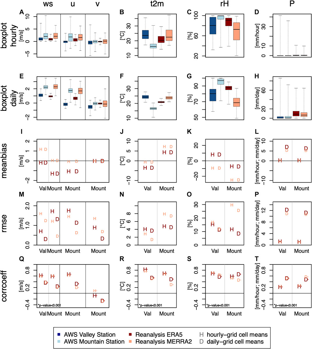
FIGURE 1. Evaluation of ERA5 and MERRA2 against both AWS (Valley Station -Val, Mountain Station -Mount) with the consideration of their distributions (A–H), mean bias (I–L), rmse (M–P), correlation coefficient (Q–T) for the variables wind speed (ws), u- and v-wind components, 2 m-temperature (t2m), relative humidity and total precipitation for the mean of the two closest grid cells to the study site based on hourly values and daily values.

The main wind direction is clearly zonally dominated. In contrast, the Valley Station is located on a north-south directed valley, which leads to more pronounced v-winds in opposition to the normally distinct u-winds. Considering the wind components of the Valley Station in the evaluation would lead to a misinterpretation, which is why they are not further considered for the mean bias, rmse and correlation analysis. The performance of both reanalysis products regarding the u-winds shows a similar bend as for the wind speed. The ERA5 median lies a bit lower than the one of the Mountain Station, whereas MERRA2 captures the range and the median of the Mountain Station quite well. Considering the mean bias (Figure 1I) and the rmse (Figure 1M), as expected, MERRA2 shows a good performance with regard to the Mountain Station.

The v-wind components are rather small, which makes it hard for reanalysis products to reproduce its variability. The resulting low correlation coefficients are of minor importance to our study due to the main wind direction along the u-axis.

In general, it should be noted that the inter-quartile range and also the whole range of values of ERA5 tends to be smaller than those of the AWS. However, considering the correlation coefficient, ERA5 performs for all wind variables (excluding v-winds) equal or even better than MERRA2 (Figure 1Q). The hourly wind correlation coefficients feature higher correlations (corr. max = 0.66) than the daily ones (corr. max = 0.37), which can be related to a well-established and well-captured daily cycle. An in-depth global evaluation of near-surface winds revealed a better performance of ERA5 in variability and also in mean winds compared to MERRA2 (Ramon et al., 2019).

Temperature

The 2 m-temperature of the Valley Station (median hourly data: 23.6°C) exceeds that of the Mountain Station (median hourly data: 16.2°C) (Figures 1B,F), due to its difference in altitude. The range of ERA5 values lies in between both AWS stations (median hourly data: 20.3°C). MERRA2 tends to reproduce the Valley Station temperatures (median hourly data: 22.6°C), which results in smaller and, in comparison to ERA5, better mean bias (Figure 1J) and rmse (Figure 1N) values with regard to the Valley Station, but higher and worse ones for the Mountain Station. As for wind speed, ERA5 reveals better correlation coefficients (Figure 1R), which implies that the variability is well captured. The existing daily cycle is represented in both reanalysis datasets.

Relative Humidity

The relative humidity of the Valley Station features generally lower values compared to the Mountain Station (Figures 1C,G). As before, ERA5 values are in the middle of both AWS, which is represented by a positive and negative mean bias for the Valley and Mountain Station, respectively (Figure 1K). MERRA2 underestimates the relative humidity on both timescales and consequently exceeds all rmse values of ERA5 (Figure 1O). The correlation coefficients are for both reanalysis quite similar with respect to the Valley Station, however, for the Mountain Station, ERA5 exhibits higher values (Figure 1S).

Precipitation

Precipitation characteristics are similar for the Valley and Mountain Stations, but both reanalysis products overestimate the amount of rain (Figures 1D,H). This becomes more obvious considering the daily sums in contrast to hourly values. For the tropical Andes, this overrating was already pointed out for MERRA2. Furthermore, precipitation in reanalysis products generally features high uncertainties, because it is not assimilated to observations (Gelaro et al., 2017). However, even high-resolution climate models tend to overestimate precipitation. This results from small conversion errors in the microphysics scheme. These accumulate with increasing amounts of liquid in clouds, which applies particularly to the tropics (Wang and Kirshbaum, 2015). In our study region, additional discrepancies arise due to missing gauge data and the high spatial variability of precipitation due to the complex mountainous topography (Lorenz and Kunstmann, 2012). Especially, the latter contributes to a scale mismatch between the reanalysis and the point measurement of the AWS, which increase the deviations (Tustison et al., 2001). Therefore, unsurprisingly, the reanalysis products have difficulties in reproducing the number of days with no rain and underestimate the amount of extreme precipitation events. However, the overall skewness of the distributions is reproduced by the reanalysis dataset. The largest difference in the correlation coefficient is found between the timescales (Figure 1T). Unlike wind and temperature, the hourly values yield smaller coefficients than the daily ones. The reason will be further investigated in section Evaluation of ERA5 Precipitation Variability.

Outcome of Evaluation of ERA5 Reanalysis Against MERRA2 and Both Automatic Weather Stations

In summary, ERA5 is more consistent in its tendency to feature values in between both AWS. Moreover, MERRA2 comprises an underestimation in relative humidity, which is undesirable for moisture source diagnostics. In contrast, ERA5 underrates the range of wind values. Nevertheless, correlation coefficients between ERA5 and AWS are in all cases (variables and timescales) almost equal or better than those between MERRA2 and the AWS. This suggests a better representation of variability within the ERA5 data for our study site.

In South America, ERA-Interim, the forerunner of ERA5 performed appropriately for different variables (Campozano et al., 2017; Montini et al., 2019; Sanabria et al., 2019) and also for trajectory analysis with and without moisture diagnostics (Knippertz et al., 2013; Drumond et al., 2014; Trachte, 2018). These studies have in common that their calculations were accomplished within the complex topography of the Andes. The higher spatial and temporal resolution of ERA5 in comparison to ERA-Interim implies a better representation of the complex topography and a reduced scale mismatch. This suggests an improvement in the precision of trajectory calculations, which is in line with Hoffmann et al. (2019). This promising behavior led us to choose ERA5 as the input dataset for our study.

Evaluation of ERA5 Precipitation Variability

Daily and Seasonal Cycle

Beginning at the daily cycle, before analyzing coarser time scales, reveals that ERA5 does not reproduce the daily cycle due to showers that occur in the afternoon instead of during the night (Figure 2A).

FIGURE 2

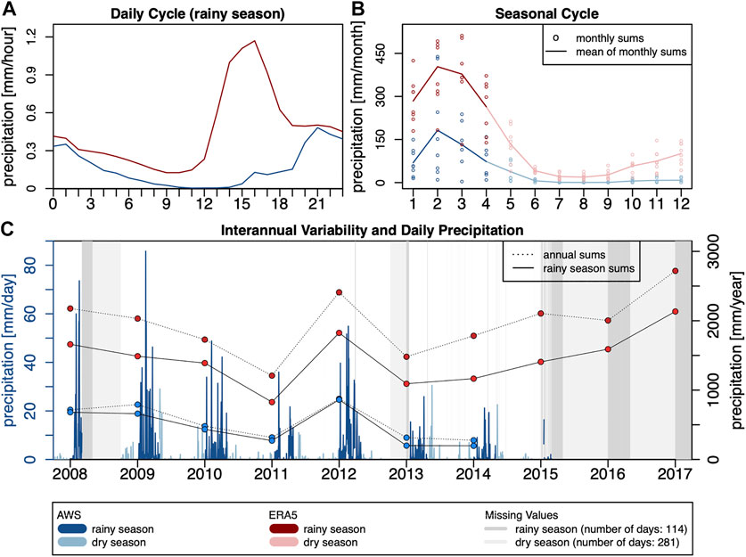
FIGURE 2. Evaluation of the variability of ERA5 (darkred) with respect to the Valley Station (blue, AWS) considering the daily (A) as well as the seasonal cycle (B) and further the rainy season and interannual variability (C).

The seasonal cycle presented as means of monthly precipitation sums is well established in ERA5 (Figure 2B). However, it is more pronounced with overestimated values during the rainy season and the beginning and the end of the dry season. During the rainy season, estimates of precipitation from reanalysis products feature the highest uncertainty, due to convective processes that are only sparsely resolved (Lorenz and Kunstmann, 2012). Moreover, ERA5 is consistent with the AWS, showing high variability within each month, in particular between January and April. The month with the greatest amount of precipitation in the AWS data is in February, whereas, ERA5 shows a maximum in March. The latter is in line with Bendix and Lauer (1992). The AWS data feature missing values in March and April 2008 (Figure 2C). As the number of years comes just to seven, we expect a bias in the monthly mean value in March and April. Moreover, the ERA5 monthly mean of February is almost as high as in March. Consequently, we determine February and March as months with maximum precipitation.

Interannual Variability

According to the interannual variability (Figure 2C), precipitation varies strongly from year to year as previous studies have already shown (Spannl et al., 2016). The years 2013 and 2014 can be classified as dry years. With respect to those, the rainfall amount is about three times higher in 2009 and 2012. In ERA5, the remarkable precipitation amount of 2012 is clearly visible. However, the reanalysis has difficulties to reproduce the dryness of 2013 and 2014. This overestimation of precipitation is not surprising, as already pointed out above. In 2008, ERA5 and AWS precipitation diverge, whereby the latter shows lower values. As the AWS measurements contain missing values for almost half of the rainy season, it can be assumed that the AWS precipitation sum for 2008 is underestimated.

The precipitation sums during the rainy season for both datasets closely follow the variability of the annual sums. On average, the rainy season contributes about 82% to the annual sum of precipitation. In 2012, this share even reached 98%. The rainy season share of ERA5 comes to 73% on average, suggesting that the overrated precipitation of the dry season is proportionally higher than for the rainy season.

Overall, the precipitation amounts in ERA5 exceed that of the AWS. As already pointed out, this overestimation is as expected. Yet, the interannual and rainy season precipitation variability is well captured. The latter was already reported for ERA-Interim with respect to the southern central Andes (Rusticucci et al., 2014). As we do not have AWS data for the years 2015–2017, we are confident in using the relative evolution of the interannual and rainy season precipitation amounts from ERA5 for further analysis. Hereby, it is important to note that rainy season precipitation amounts are steadily increasing up to 2017.

Characteristics of Precipitation Events

Two main types of precipitation can be identified in the study region, short-lasting and long-lasting events (Figure 3). The latter are frequently occurring during particularly wet years, like in 2009 (Figure 3A) and 2012 (Figure 3B). Short-lasting events occur in all years, whereby their frequencies are slightly higher in wet years.

FIGURE 3

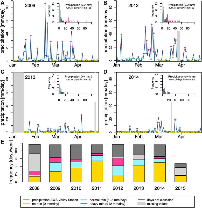
FIGURE 3. Daily precipitation of the Valley Station during the rainy seasons of the years 2009 (A), 2012 (B), 2013 (C) and 2014 (D) and its frequency distribution of all respective precipitation values above or equal 1 mm. The stacked barplot at the bottom (E) shows the year-to-year variability of the frequency of days regarding rain amount, not classified and missing values. The colors, irrespective of bars or dots, show the classes “no rain”, “normal rain” and “heavy rain.”

Besides, also dry spells may occur. This is in contrast to high intensity precipitation events that can bring up to 85 mm/day. These daily differences also exist at locations in the vicinity of our study site and show that convective activity plays an important role (Emck, 2008). Therefore, it is not surprising that many short rain events occur within our data. This kind of rain was identified as the main rain type north of our study site, close to Cuenca, Ecuador, using a vertically pointing rain radar employed from February 2017 to January 2019 (Seidel et al., 2019). These short-lasting rain events lead to moderate precipitation amounts or to heavy rain events. Convection can be attributed to an extended land-sea breeze system, but can also entrain easterlies coming from the Amazon (Bendix, 2000).

Another type of precipitation in our study region that can be associated with heavy precipitation are long-lasting events that feature durations up to a few days. They encompass high and low rainfall intensities. This phenomenon is known in this region, especially for February and March, and is related to westerly winds that can be intensified by blocking at the Andean ridge (Emck, 2008). Bendix (2000) pointed out that these persistent rains are associated with deep convection and are a result of mesoscale convective systems. The latter can spatially extend up to 250 km and are a result of atmospheric instability and high SST anomalies in the Pacific. The Paute Basin, located in the highlands of Southern Ecuador, is also influenced by mesoscale convective systems (Campozano et al., 2018).

To detect a possible relationship between the precipitation amount and moisture source regions, we generated composites of moisture source regions based on the available daily rain amount data during the rainy season from 2008 to 2015. The classification of days regarding rain amount shows a high interannual variability (Figure 3E). During the wet rainy season of the year 2012, a high number of days with heavy precipitation occurred. This is in contrast to weaker rainy seasons of the years 2011, 2013 and 2014, that show a higher number of dry days. These results are in line with the findings of the analysis of precipitation events.

Moisture Sources

Moisture sources are based on trajectory calculations and are determined by a moisture source diagnostic (see Moisture Sources based on Backward Trajectories). In our study, the determined moisture sources have to be considered as contributions in mm/day to the local precipitation. To gain confidence in the moisture source diagnostic, we evaluate it before considering the composites.

Evaluation of Moisture Source Diagnostic

The specific humidity evolution along precipitating trajectories (Figure 4) reveals that the humidity in the last few hours before reaching the starting point strongly decreases. This is reasonable, since orographic lifting due to the Andes enhances precipitation and occurs to all air masses irrespective of their origin. Apart from that, a continued increase of moisture can be observed from the end of the trajectories toward the starting point. This increase is stronger for backward times between 150 and 240 h. Test cases for two months (not shown) revealed that this increase is getting weaker beyond 240 h.

FIGURE 4

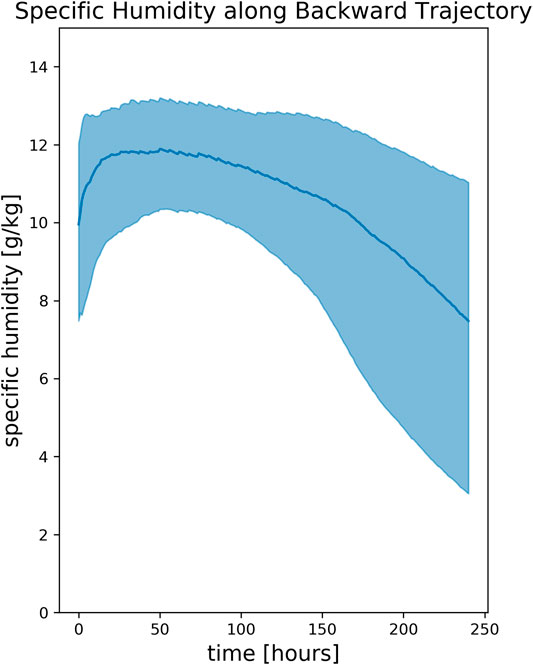
FIGURE 4. Median temporal evolution of specific humidity along the precipitating backward trajectories. The filling describes the quartiles of all values.

Daily precipitation estimates from the trajectories can reproduce the total precipitation of ERA5 (Supplementary Figure S2). Precipitation events with high amounts are mostly captured. However, the amount is usually a bit lower than that of ERA5. This can be attributed to the fact that not the whole column is considered, and the trajectories are not started every hour. The Pearson correlation coefficient comes to 0.73 and is statistically significant with a p-value < 0.001. Overall, the precipitation estimates can be considered as reasonable.

The calculated medians of the attributions (Figure 5) show a distinct pattern. With increasing height, a decreasing of the attributions below the boundary layer can be observed, as expected. At the surface, attributions are achieved mainly between 40% and 60%, while in the upper levels, the attribution reduces to around 20%. In contrast, the attributions above the boundary layer reveal attributions between 20% and 40% at the surface and high values of up to 60% in the upper levels caused by convection, turbulences, numerical diffusion and evaporation of rainwater (Sodemann et al., 2008). As convection is a main climatological process in our study area, we are not surprised having high attributions above the boundary layer. However, these are a source of uncertainty in this study that need further investigation. The year 2016 is outstanding, as almost 80% can be linked to a moisture source region (Figure 5J), whereas the attribution above the boundary layer is close to 0% (Figure 5K). An explanation would require further analysis.

FIGURE 5

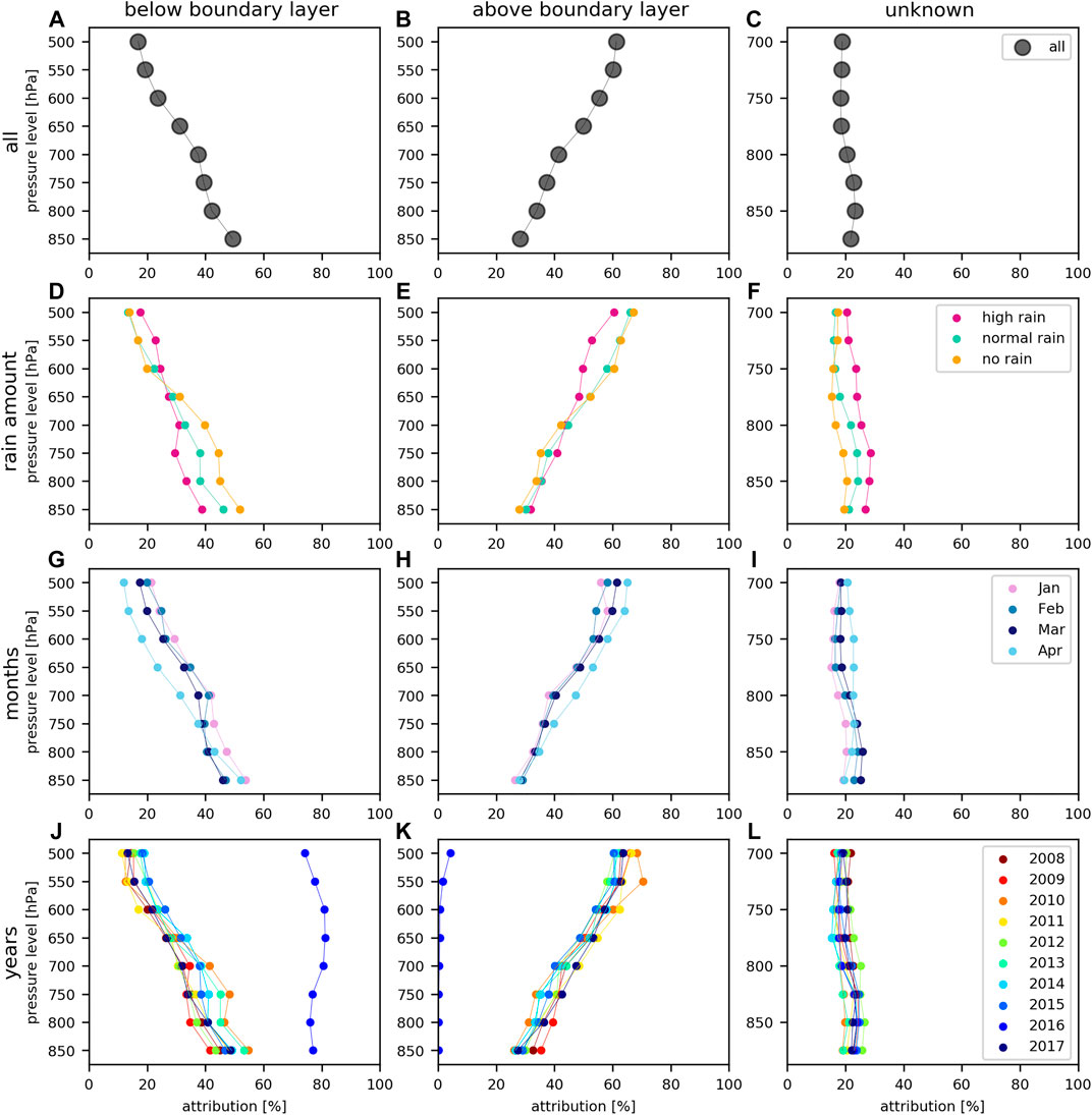
FIGURE 5. Median of trajectory attributions separated by each group (below boundary layer, above boundary layer and unknown) for each pressure level and for all values (A–C) and separated for each composite [rain amount (D–F), months (G–I), years (J–L)].

The unknown share is for all pressure levels and all composites mostly in the vicinity of 20%. For our study area, long backward time calculations are necessary due the large distance to the Atlantic. The computational expenses were, in this respect, the limiting factor. However, the best compromise between the share of unknown attributions and these expenses were found to be at a backward time of 240 h.

Composites Based on Rain Amount

Moisture sources irrespective of its composite show a clear vertical evolution (Figure 6) that can be associated with the major wind systems in that region (see Study Site). In the following, we will describe this evolution by means of the “no rain” class and will afterward point out the differences with the other classes. “No rain” moisture sources can be interpreted as humidity loss, which is not leading to the formation of precipitation (see Classification of Moisture Source Regions). These days are related to dry conditions. At 850 hPa (Figure 6G), moisture is mainly picked up from the oceanic Humboldt current, following the west coast of Peru and Ecuador, south of the study site. This southern oceanic pathway is linked to the southeasterly trade winds of the South Pacific subtropical high pressure system and was also identified by air mass trajectories for the Andes highlands in this region (Trachte, 2018). This moisture source is strongly pronounced during “no rain” days. Dry conditions in Ecuador are linked to a distinct westerly Choco Low Level Jet (Sierra et al., 2015). It evolves from the mentioned southeasterly trade winds of the eastern Pacific and recurves to westerlies at 5°N (Poveda and Mesa, 2000; Amador et al., 2006). Consequently, intense southeasterly trade winds off the coast of Ecuador lead to dry conditions in our study area. However, its influence decreases with height.

FIGURE 6

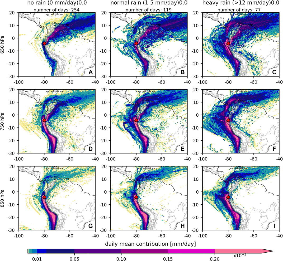
FIGURE 6. Moisture source regions given as daily mean contribution (mm/day) to the precipitation at the study site for the pressure levels 850, 750 and 650 hPa and separated into the composites of rain amount (“no rain” (A,D,G), “normal rain” (B,E,H) and “heavy rain” (C,F,I). Topographic contours, with 750 m interval, shown as gray lines.

Easterly trade winds begin to dominate at higher levels, as the blocking by the Andes declines (Figures 6A,D). Thereby, two continental moisture source branches can be identified, a very weak southern branch and a distinct northern one. The southern continental branch obtains moisture from the eastern flanks of the Peruvian and Bolivian Andes and Brazil. However, no such trajectory pathway is existent in the study for the Andes highlands (Trachte, 2018). The reason could be that it is disregarded in their applied factor analysis due to its low intensity and moreover, due to the differing location. The northern one, is very pronounced and gains humidity from the eastern flanks of the Colombian Andes and along the Orinoco plains “Los Llanos” covering parts of Colombia and Venezuela. At 650 hPa (Figure 6A), the majority of moisture is originating from these plains. This is in line with the results of a trajectory analysis for the Andes highlands (Trachte, 2018).

“Heavy rain” moisture sources show differing characteristics from those of “no rain” at all considered levels (Figures 6C,F,I). At 850 hPa (Figure 6I), the importance of the southern oceanic source region has decreased. In accordance, moisture is picked up from the ocean west of the study site and to the north. The latter exhibits regions within the Pacific Ocean, like the Gulf of Panama, and even the Caribbean Sea. These additional oceanic western and northern uptake regions are existent throughout the other pressure levels. The enhanced westerlies during heavy precipitation events (Bendix, 2000) can therefore be linked to an increase of ocean moisture source regions west and north of the study site and a decrease in moisture input from westerlies arising from the recurved southerlies. This is reasonable, since heavy precipitation events are often related to a weaker South Pacific subtropical surface high pressure system and less ascending air (Endlicher et al., 1989; Bendix and Lauer, 1992), which in turn allows an approaching of air masses from the north to the study region (Bendix and Lauer, 1992).

As convection is another process leading to heavy precipitation (see Characteristics of Precipitation Events), it is not surprising that an enhanced local uptake of moisture can be identified. This can be seen at all pressure levels (Figures 6C,F,I), but mainly at 650 hPa (Figure 6I).

“Normal rain” moisture sources feature regions that describe a mixture of “no rain” and “heavy rain” ones (Figures 6B,E,H). In particular, at each pressure level, a westerly influence is visible, though it is not as distinct as for “heavy rain.” The same applies to the oceanic moisture source region from the Caribbean.

In summary, at the lower levels, moisture is mainly picked up along the South American coast south of the study site, whereas, with increasing height, northern South America and the Atlantic are the main sources of moisture. “Heavy rain” days in contrast to “no rain” days show a strongly enhanced oceanic moisture uptake west and north of the study site, even reaching the Caribbean Sea.

Composites for Each Month (2008–2017)

Moisture source regions show a different pattern over the course of the rainy season (Figure 7).

FIGURE 7

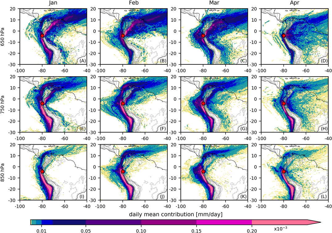
FIGURE 7. As Figure 6, but for the composites of each month [January (A,E,I), February (B,F,J), March (C,G,K), April (D,H,L)].

The oceanic influence from the Caribbean Sea exists throughout the considered atmospheric pressure levels. It reaches its maximum in February (Figures 7B,F,J) and decreases toward April (Figures 7D,H,L).

The oceanic moisture source region west of the study site is most pronounced in February and March (Figures 7B,F,J,C,G,K) at all pressure levels, which coincides with the two months of maximum precipitation.

The southern oceanic influence is most distinct in January (Figures 7A,E,I) and re-strengthens in April. It is the main feature at the 850 hPa level in all months and loses its importance with increasing height.

The continental northern branch sticks, in January, mostly to the Orinoco plains (Figures 7A,E). With proceeding months, moisture is increasingly picked up in regions further south, resulting in moisture regions in April that extend from the northeastern flanks of the Andes over the majority of the northern continent (Figures 7D,H). This applies mostly to the upper two pressure levels considered in this study. Such a shift was also found in other studies (Drumond et al., 2014; Trachte, 2018). In particular, trajectory analysis for the Amazon Basin revealed that during the austral summer, moisture is picked up predominantly in the tropical North Atlantic, while during the austral winter, the main source region is restricted to the South Atlantic (Drumond et al., 2014).

The observed spreading of moisture sources over the continent toward the end of the rainy season can, therefore, be interpreted as transition to the austral winter moisture source regions in the South Atlantic. This coincides with the manifestation of the continental source region to the south. It is not existent in February at 750 and 650 hPa (Figures 7B,F) while it is most pronounced in April (Figures 7D,H).

The findings of Drumond et al. (2014) additionally confirm the decreasing influence of the Caribbean moisture source over the course of the rainy season, as this region is part of the tropical North Atlantic. These results are maintained if the years 2016 and 2017 are excluded, which were exceptional within the analysis time period due to El Niño events (Supplementary Figure S3, see Sea Surface Temperature).

Composites for Each Calendar Year

The interannual change of moisture sources during the rainy season was analyzed by considering all calculated pressure levels together for each year (Figure 8).

FIGURE 8

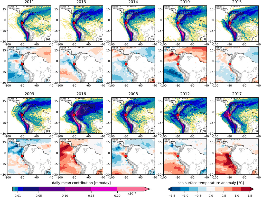
FIGURE 8. Moisture source regions given as daily mean contribution (mm/day) to the precipitation at the study site for all calculated pressure levels and separated into the composites of each year (2008–2017) (A–E,K–O). The rainy season precipitation sums increase from the upper left plot to the lower right one. Every second row shows sea surface temperature anomalies (F–J,P–T) with respect to the time period from 2008 to 2017. Topographic contours, with 750 m interval, shown as gray lines.

Increasing rainy season precipitation amounts reveal an enhanced influence of the moisture source region west of the study site, which is in line with previous findings of this study.

The most intense contribution from the Caribbean Sea can be observed during years with high precipitation sums (2016, 2017, Figures 8L,O), whereas the weakest manifestation is linked to the years with the lowest amounts (2011, 2013, Figures 8A,B). However, less pronounced contributions from this branch could also occur during wet years (2012, Figure 8N). Since these results are still inconclusive, we suggest that other processes are of higher importance for contributing to the observed interannual differences. The same applies to the continental branches, which do not reveal any specific pattern.

Sea Surface Temperature

The central tropical Pacific showed neutral to cold conditions during the rainy seasons of 2011, 2013 and 2014 (Santoso et al., 2017). The same applies to the eastern Pacific off the coast of Ecuador (Figures 8F–H). These years are related to low rainy season precipitation amounts and lack distinct moisture sources west of the study site (Figures 8A–C). This also applies to 2010 (Figure 8D), however, in this year a central Pacific El Niño occurred (Lee and McPhaden, 2010; Santoso et al., 2017; Wang et al., 2017) leaving the eastern tropical Pacific in cold conditions (Figure 8I). The situation is similar to 2015 (Santoso et al., 2017), but the moisture source region west of the study site is more pronounced in 2015 (Figure 8E). This might be due to a warming starting toward the end of the rainy season (McPhaden, 2015). Although warm conditions prevailed in the central Pacific, the precipitation amount of the rainy season was moderate.

The year 2016 was exceptional, as it is related to a major eastern Pacific El Niño event (L’Heureux et al., 2017; Sanabria et al., 2019). During the rainy season, the mean evaporative moisture uptake reveals extraordinarily high values in the whole region (Figure 8L). The continental as well as the oceanic moisture source regions contribute to precipitation at our study site. Moisture transport analyses discovered that the moisture in 2016 originated from both sides of the Andes (Sanabria et al., 2019).

2017 is the wettest of the considered rainy seasons. Although the moisture sources are not as extensive as in 2016, the contribution of the oceanic source region west of the study site is more intense and more concentrated on the coast (Figure 8O). The same applies to the SSTs, that are linked to a coastal El Niño event (Echevin et al., 2018; Garreaud, 2018; Rodriguez-Morata et al., 2019). This suggests a greater importance of coastal SST anomalies instead of those occurring closer to the central Pacific. Additionally, this event can be linked to a decreased intensity of southeasterly trade winds and enhanced northwesterly winds (Garreaud, 2018). The associated warm SSTs, that reached 28°C along the Peruvian coasts during March 2017 (Rodriguez-Morata et al., 2019), led to deep convection (Garreaud, 2018; Rodriguez-Morata et al., 2019). In accordance, moisture is extensively taken up in the vicinity of our study site.

The moisture source region patterns west of the study site in 2008 and 2012 (Figures 8M,N) are similar to those in 2017, however, markedly less distinct and reaching slightly further west. These two years do not show as intensive warming as in 2016 and 2017, but have a strong very localized warm SST anomaly, which occurred off the coast of Ecuador (Figures 8R,S). The rest of the tropical Pacific in 2008 showed cold anomalies (Bendix et al., 2011). Similarly, in the beginning of 2012, cold La Niña conditions were decaying in the central Pacific, while a warming occurred in the eastern Pacific (Su et al., 2014) (Figure 8).

These results further indicate that irrespective of their extent, warm SST anomalies near the Ecuadorian coast are more effective in increasing the western oceanic moisture uptake for the study site than warm SST anomalies in the central Pacific. This confirms the findings of other studies pointing to the importance of local SSTs for the generation of rain events on the western flanks of the Ecuadorian Andes (Bendix et al., 2011; Vicente-Serrano et al., 2017).

Further, Drumond et al. (2014) found out that the Amazon receives enhanced moisture input from the North Atlantic during La Niña years. In contrast, during El Niño years, the main moisture source is the South Atlantic. Our results regarding the moisture coming from the Amazon Basin also show such a tendency, but it is not clearly visible. This may be related to the few cases for El Niño and La Niña events that occurred during our study period.

In summary, with rising precipitation amounts, moisture is increasingly picked up from the ocean west of the study site. This can also be seen over the course of the rainy season and in years with high rainy season precipitation sums. This moisture source region can be further associated with local warm SST anomalies in the eastern Pacific. However, in each case, the study site shows influences from both, the oceanic tropical Pacific and the continental Amazon.

Hydroclimatic Controls on δ¹⁸O in Tree Rings

In the following, we discuss possible climatic mechanisms affecting the δ¹⁸O variability in tree rings of Bursera graveolens, like rain amount and its moisture source regions.

The interpretation of the seasonally resolved tree-ring isotope values needs to be taken with caution, since the individual values are not absolutely dated, due to missing information of the beginning and end of the growing season of Bursera graveolens. A study that analyzed tree ring widths of Bursera graveolens pointed out that much of the tree growth occurred after rain events, which fall between January and March/April (Rodríguez et al., 2005). The same was found for other tree species in our study area (Butz et al., 2017). However, another study found significant correlations between tree ring width of Bursera graveolens and regional precipitation from February until June and in September (Pucha-Cofrep et al., 2015). Therefore, we suggest that further investigations, like dendrometer measurements or cambial monitoring, are necessary to precisely date the growing season. Furthermore, the first and last few values of a year may contain a mixed signal of two years, since the annual tree-ring boundaries where not always perpendicular on the collected increment cores. Despite of these limitations, we undertook the effort to evaluate the impact of precipitation events and changes in moisture sources on the intra-annual variations of δ¹⁸O in tree rings of Bursera graveolens.

A distinct and stable seasonal cycle of isotopic values is not evident (Figures 9A,B,D,E,F), as it was found in a temperate forest in North America, where seasonal temperature variations and precipitation deficit were identified as the driving mechanisms (Evans and Schrag, 2004). However, since temperature does not vary strongly at our study site (Pucha-Cofrep et al., 2015), we do not expect a great influence of temperature on δ¹⁸O variations. In line with our findings, tree ring δ¹⁸O variations in Prosopis sp. in northwestern Peru, about 100 km south of our study site, did not reveal a seasonal cycle (Evans and Schrag, 2004). Nevertheless, some temporal patterns can be recognized in the δ¹⁸O variations in Bursera graveolens. In 2012 and 2013 (Figures 9A,B), increasing δ¹⁸O values at the beginning of the growing season lead to a first maximum, that is followed by a minimum and a second maximum before decreasing at the end of the growing season. In 2017 (Figure 9F), the course of the isotopes is similar, but starts with the decreasing part toward the minimum. In contrast, isotope values in 2016 (Figure 9E) do not show a clear temporal pattern, although a minimum and a following maximum with decreasing values toward the end of the growing season can be identified. For 2015 (Figure 9D), no particular pattern is visible.

FIGURE 9

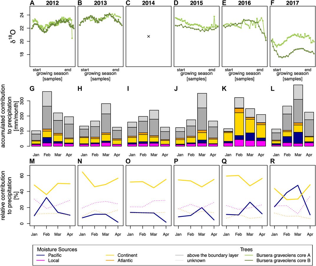
FIGURE 9. Tree ring isotopes of Bursera graveolens for each year, the values are linearly distributed within the growing season, since a seasonal dating was not possible (A–F). In 2014, no tree ring was built (C). Accumulated moisture contributions from different regions (G–L). Relative moisture contributions from different regions (M–R). Moisture contributions are based on the precipitation estimates derived from the trajectories.

The increasing isotope trend in the beginning of the growing seasons of 2012 and 2013 fits with the rising relative moisture source contribution from the Pacific and a coupled decreasing influence from the continent during January and February (Figures 9M,N). Moisture from the Pacific exhibits relatively enriched values of δ¹⁸O due to its short moisture transport pathway to the study site and the resulting small fractionation processes. In contrast, the continental signal is depleted in δ¹⁸O. We suggest that this rising influence from the Pacific leads to the increasing δ¹⁸O values in the beginning of the growing season. As indicated, these Pacific moisture contributions are related to heavy precipitation events. These occur and lead to high precipitation amounts. The latter are evident in the rising accumulated contributions toward February and March based on the precipitation estimates from the trajectories (Figures 9G,H). As a result, the rain amount effect sets in, which leads to the observed decreasing δ¹⁸O values. The decreasing δ¹⁸O pattern at the end of the growing season can be related to a decreasing moisture contribution from the Pacific and an enhanced moisture contribution from the continent. In 2015 and 2016 (Figures 9P,Q), this changing relative moisture source contribution begins quite late in the growing season, explaining why this effect might be overlaid in the isotopic signal by other mechanisms. In 2017 (Figure 9R), the moisture source contribution from the Pacific is already pronounced in January. Due to the early onset of the increasing influence of the Pacific, the increasing δ¹⁸O signal might not be recorded as the growing season sets in later. The effect of changing moisture sources on the isotopic composition of climate proxies has been demonstrated on an annual basis in different studies and regions (Wernicke et al., 2016; Grießinger et al., 2018), but was also shown for a seasonally resolved proxy (Muangsong et al., 2020).

The annual course of the isotopic values from 2012 to 2017 is quite pronounced, 2017 stands out with values as low as about 18‰ (Figure 9F). In comparison, the values of the other years range from 22–24‰ (Figures 9A,B,D,E). In contrast, the highest δ¹⁸O values were recorded in 2013 (Figure 9B). In 2014 (Figure 9C), no interpretable tree ring has formed, since it is the second dry year in a row.

The rain amount of the rainy season does have an effect on the isotopic values, which is known as the amount effect (Dansgaard, 1964). This is particularly obvious in 2017 and 2013, the years with the lowest and highest δ¹⁸O values. They are linked to the wettest and one of the driest years, respectively. As indicated, the high precipitation amounts of 2017 can be linked to a coastal El Niño event. A strong decrease in δ¹⁸O was also observed in Prosopis sp. tree rings in northwestern Peru during the eastern Pacific El Niño in 1998 and was also accompanied by high precipitation amounts (Evans and Schrag, 2004). Furthermore, the oxygen isotope signature of teak trees (Tectona grandis) from Java revealed a negative correlation with rain amounts during the dry and rainy season as well and also record ENSO related signals (Schollaen et al., 2013; Schollaen et al., 2015). However, during the very wet rainy season of 2016 which can be directly linked to a major eastern Pacific El Niño (L’Heureux et al., 2017; Sanabria et al., 2019), the isotope ratios do not show a strong drop. Particularly low δ¹⁸O values would be expectable due to the additional effect of the enhanced continental influence. Local recycling, where moisture is reentering the atmosphere by evaporation is an important process within the Amazon Basin (Victoria et al., 1991; Eltahir and Bras, 1994). This mechanism, which would result in a mixed isotopic signal, might explain the unexpected isotopic ratios of 2016.

It also needs to be kept in mind, that the δ¹⁸O variations in tree rings partly represent the δ¹⁸O changes of soil water. This means that the δ¹⁸O composition of rain undergoes further fractionation processes from the soil surface to the root depth. Additionally, tree physiological mechanisms, like leaf water enrichment further control the isotopic composition (Gat, 1996; McCarroll and Loader, 2004; Gessler et al., 2014; van der Sleen et al., 2017).

To increase the understanding of the isotopic signal in particular with respect to local processes, also changes of temperature, local precipitation and relative humidity need to be taken into account. For the latter two variables, no daily dataset was available to represent the local variability for the years 2016 and 2017 (not covered by the AWS data) appropriately (not shown). Temperature was neglected in our study, since it does not vary strongly over the course of the year.

Additional uncertainty is added by the scale mismatch between the local isotopic signal of the tree and the calculated moisture sources based on the ERA5 reanalysis (Ludwig et al., 2018), as applies for the comparison between the AWS and the reanalysis datasets.

Furthermore, due to dating uncertainties in some of the analyzed intra-annually isotope time series, the number of two δ¹⁸O reliably dated time series is not yet representative for a thorough analysis. Therefore, the results serve as discussion basis that warrants further investigation. A higher sampling replication for the corresponding period are envisaged as part of a future study.

Conclusions

In this study, we calculated moisture source regions for our study site in southern Ecuador on the western flanks of the Andes by using the trajectory model LAGRANTO and related those to precipitation events. We further analyzed the seasonal and annual evolution of the moisture sources and discussed possible relationships with seasonally resolved oxygen isotope ratios of tree rings of Bursera graveolens. ERA5 served as input dataset for LAGRANTO, whereas AWS data were utilized to analyze precipitation events. The main outcomes of our study encompass:

(1) Heavy precipitation events reveal a high moisture contribution from the Pacific.

(2) Warm coastal Pacific SST anomalies are more important for heavy precipitation events than warmings off the coast or in the central Pacific.

(3) Precipitation at the study site consists of a mixture of moisture from the Pacific and from continental areas east of the Andes as far as the Atlantic Ocean—however the relative contribution is variable throughout the rainy season, with particularly enhanced contributions from the Pacific in February and March.

(4) The isotopic signatures of Bursera graveolens witnesses precipitation amount effects and reflects the changes in the relative contribution of moisture source regions over the course of the rainy season.

The outcome of this study can contribute to a better understanding and higher confidence in the hydrological processes that influence the study site and emphasize that both the Pacific as well as continental South America and the Atlantic contribute to its precipitation.

The gained knowledge about moisture sources and the discussed relationship to the isotopic signature of Bursera graveolens is a good basis for future work.

Questions that remain to be answered are

(1) Why are the δ¹⁸O values in 2016 unexpectedly high, although the rain amount is among the highest within the analyzed ten-year period beside an exceptionally high continental contribution?

(2) How is the considerable attribution of moisture uptake above the boundary layer height influencing the isotopic signal?

(3) Can we achieve a precise dating of the intra-annual tree ring δ¹⁸O values and find further confidence in the postulated argumentation regarding the change of relative contribution of the moisture sources?

To address these open questions, we plan to employ a high-resolution atmospheric model in the next step, which will allow us to investigate the influence of convection and other local or mesoscale processes on the isotopic signal. Taking into account that convection is not captured with the applied moisture source diagnostic but leads to a high attribution amount above the boundary layer height, it might be a key factor in answering the first two questions. This argument is particularly valid, as convection is one of the main processes at the study site. Additionally, this approach will help us to resolve the scale mismatch. We will use an isotope-enabled version of the model to gain better knowledge about the isotopic composition of precipitation in the study area and how it is modified by convection. This might provide a possibility to seasonally date the isotopic ratios of Bursera graveolens and find further proof of the hypothesized influence of moisture sources on the seasonal isotopic ratio. For the latter, further intra-annual tree ring isotope series with precise dating control through associated measurements of tree ring growth and cambial modeling are inevitable.

Data Availability Statement

The raw data supporting the conclusions of this article will be made available by the authors, without undue reservation.

Author Contributions

NL: Performed the trajectory and moisture source calculations as well as the data analyses, created the plots and drafted the manuscript. TM supervised the project. NL, TM, JG and TP contributed to the conception and design of the study. NL, JG and AB completed the stable isotope analyses. All authors contributed to the article and approved the submitted version.

Funding

This study was funded by the Friedrich-Alexander-Universität Erlangen-Nürnberg.

Conflict of Interest

The authors declare that the research was conducted in the absence of any commercial or financial relationships that could be construed as a potential conflict of interest.

Acknowledgments

The authors thank Volker Raffelsbauer for the collection of the Bursera graveolens tree cores and Iris Burchardt and Roswitha Höfner-Stich for the processing of the oxygen isotopes. Further, we acknowledge the provision of the AWS data that benefited from the financial support granted by the German Science Foundation (DFG project code BR1895/29-1) within research unit 2730 RESPECT. For data provision of ERA5, we thank the European Centre for Medium-Range Weather Forecasts. The High Performance Computing Centre (HPC) at the University of Erlangen- Nürnberg’s Regional Computation Center (RRZE), we acknowledge for the supply of the resources to store and process all data of the trajectory calculation. We thank Darwin Alexander Pucha Cofrep (Universidad Nacional de Loja, Ecuador) for collaboration and we thank the Ecuadorian Ministry of the Environment (MAE) for the research permission and Nature and Culture International (NCI) for logistic support. Finally, we want to thank the editor R. Nieto and the two reviewers for their helpful comments.

Supplementary Material

The Supplementary Material for this article can be found online at: https://www.frontiersin.org/articles/10.3389/feart.2020.604804/full#supplementary-material.

References

Alduchov, O. A., and Eskridge, R. E. (1996). Improved magnus form approximation of saturation vapor pressure. J. Appl. Meteorol. 35 (4), 601–609. doi:10.1175/1520-0450(1996)035<0601:Imfaos>2.0.Co

CrossRef Full Text | Google Scholar

Amador, J. A., Alfaro, E. J., Lizano, O. G., and Magana, V. O. (2006). Atmospheric forcing of the eastern tropical Pacific: a review. Prog. Oceanogr. 69 (2–4), 101–142. doi:10.1016/j.pocean.2006.03.007

CrossRef Full Text | Google Scholar

Bendix, A., and Bendix, J. (2006). Heavy rainfall episodes in Ecuador during El Niño events and associated regional atmospheric circulation and SST patterns. Adv. Geosci. 6. doi:10.5194/adgeo-6-43-2006

CrossRef Full Text | Google Scholar

Bendix, J., Gaemmerler, S., and Reudenbach, C. (2003). A case study on rainfall dynamics during El Niño/La Niña 1997/99 in Ecuador and surrounding areas as inferred from GOES-8 and TRMM-PR observations. Erdkunde 57 (2), 81–93. doi:10.3112/erdkunde.2003.02.01

CrossRef Full Text | Google Scholar

Bendix, J., and Lauer, W. (1992). Die Niederschlagsjahreszeiten in Ecuador und ihre klimadynamische Interpretation. Erdkunde 46, 118–134. doi:10.3112/erdkunde.1992.02.04

CrossRef Full Text | Google Scholar

Bendix, J. (2000). Precipitation dynamics in Ecuador and northern Peru during the 1991/92 El Niño: a remote sensing perspective. Int. J. Rem. Sens. 21 (3), 533–548. doi:10.1080/014311600210731

CrossRef Full Text | Google Scholar

Bendix, J., Trachte, K., Palacios, E., Rollenbeck, R., Goettlicher, D., Nauss, T., et al. (2011). El Niño meets La Niña-anomalous rainfall patterns in the “traditional” El Niño region of southern Ecuador. Erdkunde 65 (2), 151–167. doi:10.3112/erdkunde.2011.02.04

CrossRef Full Text | Google Scholar

Braeuning, A. (2009). Climate variability of the tropical Andes since the late Pleistocene. Adv. Geosci. 22. doi:10.5194/adgeo-22-13-2009

CrossRef Full Text | Google Scholar

Butz, P., Raffelsbauer, V., Graefe, S., Peters, T., Cueva, E., Holscher, D., et al. (2017). Tree responses to moisture fluctuations in a neotropical dry forest as potential climate change indicators. Ecol. Indicat. 83, 559–571. doi:10.1016/j.ecolind.2016.11.021

CrossRef Full Text | Google Scholar

Campozano, L., Trachte, K., Celleri, R., Samaniego, E., Bendix, J., Albuja, C., et al. (2018). Climatology and teleconnections of mesoscale convective systems in an Andean basin in southern Ecuador: the case of the Paute Basin. Adv. Meteorol. 2018, 1–13. doi:10.1155/2018/4259191

CrossRef Full Text | Google Scholar

Campozano, L., Vazquez-Patino, A., Tenelanda, D., Feyen, J., Samaniego, E., and Sanchez, E. (2017). Evaluating extreme climate indices from CMIP3&5 global climate models and reanalysis data sets: a case study for present climate in the Andes of Ecuador. Int. J. Climatol. 37, 363–379. doi:10.1002/joc.5008

CrossRef Full Text | Google Scholar

Capotondi, A., Wittenberg, A., Newman, M., Lorenzo, E. D., Yu, J. Y., Braconnot, P., et al. (2015). Understanding ENSO diversity. Bull. Am. Meteorol. Soc. 96 (6), 921–938. doi:10.1175/BAMS-D-13-00117.1

CrossRef Full Text | Google Scholar

Copernicus Climate Change Service [C3S] (2017). ERA5: fifth generation of ECMWF atmospheric reanalysis of the global climate. Copernicus climate change Service data store (CDS) [Online]. Available at: http://cds.climate.copernicus.eu/cdsapp#!/home (Accessed 11 February, 2020).

Google Scholar

Crawford, J., Hughes, C. E., and Parkes, S. D. (2013). Is the isotopic composition of event based precipitation driven by moisture source or synoptic scale weather in the Sydney Basin, Australia? J. Hydrol. 507, 213–226. doi:10.1016/j.jhydrol.2013.10.031

CrossRef Full Text | Google Scholar

Dansgaard, W. (1964). Stable isotopes in precipitation. Tellus 16, 436–468. doi:10.3402/tellusa.v16i4.8993

CrossRef Full Text | Google Scholar

Dee, D. P., Uppala, S. M., Simmons, A. J., Berrisford, P., Poli, P., Kobayashi, S., et al. (2011). The ERA-Interim reanalysis: configuration and performance of the data assimilation system. Q. J. R. Meteorol. Soc. 137 (656), 553–597. doi:10.1002/qj.828

CrossRef Full Text | Google Scholar

Drumond, A., Marengo, J., Ambrizzi, T., Nieto, R., Moreira, L., and Gimeno, L. (2014). The role of the Amazon Basin moisture in the atmospheric branch of the hydrological cycle: a Lagrangian analysis. Hydrol. Earth Syst. Sci. 18 (7), 2577–2598. doi:10.5194/hess-18-2577-2014

CrossRef Full Text | Google Scholar

Echevin, V., Colas, F., Espinoza-Morriberon, D., Vasquez, L., Anculle, T., and Gutierrez, D. (2018). Forcings and evolution of the 2017 coastal El Niño off Northern Peru and Ecuador. Front. Marine Sci. 5. doi:10.3389/fmars.2018.00367

CrossRef Full Text | Google Scholar

Eltahir, E. A. B., and Bras, R. L. (1994). Precipitation recycling in the Amazon Basin. Q. J. R. Meteorol. Soc. 120 (518), 861–880. doi:10.1256/smsqj.51805

CrossRef Full Text | Google Scholar

Emck, P. (2008). A climatology of south Ecuador: with special focus on the major andean climate divide. Saarbrücken, Germany: VDM Verlag.

Google Scholar

Endlicher, W., Habbe, K. A., and Pinzner, H. (1989). Zum EI Niño-Southern Oscillation-Ereignis 1983 und seinen Auswirkungen im peruanischen Küstengebiet. Mitteilungen Fränkischen Geographischen Gesellschaft 36, 174–201.

Google Scholar

Evans, M. N., and Schrag, D. P. (2004). A stable isotope-based approach to tropical dendroclimatology. Geochem. Cosmochim. Acta 68 (16), 3295–3305. doi:10.1016/j.gca.2004.01.006

CrossRef Full Text | Google Scholar

Garreaud, R. D. (2018). A plausible atmospheric trigger for the 2017 coastal El Niño. Int. J. Climatol. 38, E1296–E1302. doi:10.1002/joc.5426

CrossRef Full Text | Google Scholar

Gat, J. R. (1996). Oxygen and hydrogen isotopes in the hydrologic cycle. Annu. Rev. Earth Planet Sci. 24, 225–262. doi:10.1146/annurev.earth.24.1.225

CrossRef Full Text | Google Scholar

Gelaro, R., McCarty, W., Suarez, M. J., Todling, R., Molod, A., Takacs, L., et al. (2017). The Modern-Era retrospective analysis for research and applications, version 2 (MERRA-2). J. Clim. 30 (14), 5419–5454. doi:10.1175/Jcli-D-16-0758.1

CrossRef Full Text | Google Scholar

Gessler, A., Ferrio, J. P., Hommel, R., Treydte, K., Werner, R. A., and Monson, R. K. (2014). Stable isotopes in tree rings: towards a mechanistic understanding of isotope fractionation and mixing processes from the leaves to the wood. Tree Physiol. 34 (8), 796–818. doi:10.1093/treephys/tpu040

PubMed Abstract | CrossRef Full Text | Google Scholar

Grießinger, J., Langhamer, L., Schneider, C., Sass, B. L., Steger, D., Skvarca, P., et al. (2018). Imprints of climate signals in a 204 Year delta O-18 Tree-Ring Record of Nothofagus pumilio from Perito Moreno glacier, southern Patagonia (50 degrees S). Front. Earth Sci. 6. doi:10.3389/feart.2018.00027

CrossRef Full Text | Google Scholar

Hersbach, H., Bell, B., Berrisford, P., Horányi, A., Muñoz-Sabater, C., Nicolas, J., et al. (2019). Global reanalysis: goodbye ERA-Interim, hello ERA5. ECMWF Newlett. 159, 17–24.

Google Scholar

Hersbach, H., de Rosnay, P., Bell, B., Schepers, D., Simmons, A., Soci, C., et al. (2018). Operational global reanalysis: progress, future directions and synergies with NWP. ERA Report Series 27 (Accessed December 2018).

Google Scholar

Hoffmann, L., Gunther, G., Li, D., Stein, O., Wu, X., Griessbach, S., et al. (2019). From ERA-Interim to ERA5: the considerable impact of ECMWF's next-generation reanalysis on Lagrangian transport simulations. Atmos. Chem. Phys. 19 (5), 3097–3124. doi:10.5194/acp-19-3097-2019

CrossRef Full Text | Google Scholar

Horel, J. D., and Cornejogarrido, A. G. (1986). Convection along the coast of northern Peru during 1983 - spatial and temporal variation of clouds and rainfall. Mon. Weather Rev. 114 (11), 2091–2105. doi:10.1175/1520-0493(1986)114<2091:Catcon>2.0.Co

CrossRef Full Text | Google Scholar

Jana, S., Rajagopalan, B., Alexander, M. A., and Ray, A. J. (2018). Understanding the dominant sources and tracks of moisture for summer rainfall in the southwest United States. J. Geophys. Res. -Atmos. 123 (10), 4850–4870. doi:10.1029/2017jd027652

CrossRef Full Text | Google Scholar

Jones, P. D., Briffa, K. R., Osborn, T. J., Lough, J. M., van Ommen, T. D., Vinther, B. M., et al. (2009). High-resolution palaeoclimatology of the last millennium: a review of current status and future prospects. Holocene 19 (1), 3–49. doi:10.1177/0959683608098952

CrossRef Full Text | Google Scholar

Kieslinger, J., Pohle, P., Buitron, V., and Peters, T. (2019). Encounters between experiences and measurements: the role of local knowledge in climate change research. Mt. Res. Dev. 39 (2), R55–R68. doi:10.1659/Mrd-Journal-D-18-00063.1

CrossRef Full Text | Google Scholar

Knippertz, P., Wernli, H., and Glaser, G. (2013). A global climatology of tropical moisture exports. J. Clim. 26 (10), 3031–3045. doi:10.1175/Jcli-D-12-00401.1

CrossRef Full Text | Google Scholar

L’Heureux, M. L., Takahashi, K., Watkins, A. B., Barnston, A. G., Becker, E. J., Di Liberto, T. E., et al. (2017). Observing and predicting the 2015/16 El Niño. Bull. Am. Meteorol. Soc. 98 (7), 1363–1382. doi:10.1175/Bams-D-16-0009.1

CrossRef Full Text | Google Scholar

Langhamer, L., Sauter, T., and Mayr, G. J. (2018). Lagrangian detection of moisture sources for the southern Patagonia icefield (1979–2017). Front. Earth Sci. 6. doi:10.3389/feart.2018.00219

CrossRef Full Text | Google Scholar

Lee, T., and McPhaden, M. J. (2010). Increasing intensity of El Niño in the central-equatorial pacific. Geophys. Res. Lett. 37. doi:10.1029/2010gl044007

CrossRef Full Text | Google Scholar

Lorenz, C., and Kunstmann, H. (2012). The hydrological cycle in three state-of-the-art reanalyses: intercomparison and performance analysis. J. Hydrometeorol. 13 (5), 1397–1420. doi:10.1175/Jhm-D-11-088.1

CrossRef Full Text | Google Scholar

Ludwig, P., Gomez-Navarro, J. J., Pinto, J. G., Raible, C. C., Wagner, S., and Zorita, E. (2018). Perspectives of regional paleoclimatie modeling. Ann. N. Y. Acad. Sci. 1436 (1), 54–69. doi:10.1111/nyas.13865

PubMed Abstract | CrossRef Full Text | Google Scholar

McCarroll, D., and Loader, N. J. (2004). Stable isotopes in tree rings. Quat. Sci. Rev. 23 (7–8), 771–801. doi:10.1016/j.quascirev.2003.06.017

CrossRef Full Text | Google Scholar

McPhaden, M. J. (2015). Commentary: playing hide and seek with El Niño. Nat. Clim. Change 5 (9), 791–795. doi:10.1038/nclimate2775

CrossRef Full Text | Google Scholar

McPhaden, M. J., Zebiak, S. E., and Glantz, M. H. (2006). ENSO as an integrating concept in Earth science. Science 314 (5806), 1740–1745. doi:10.1126/science.1132588

PubMed Abstract | CrossRef Full Text | Google Scholar

Meier, W. J. H., Araven, J. C., Jañac, R., Braun, M. H., Hochreuther, P., Soto-Rogela, P., et al. (2020). A tree-ring δ18O series from southernmost Fuego-Patagonia is recording flavors of the Antarctic Oscillation. Global Planet. Change 195. doi:10.1016/j.gloplacha.2020.103302

CrossRef Full Text | Google Scholar

Moelg, T., Chiang, J. C. H., Gohm, A., and Cullen, N. J. (2009). Temporal precipitation variability versus altitude on a tropical high mountain: observations and mesoscale atmospheric modelling. Q. J. R. Meteorol. Soc. 135 (643), 1439–1455. doi:10.1002/qj.461

CrossRef Full Text | Google Scholar

Moelg, T., and Kaser, G. (2011). A new approach to resolving climate-cryosphere relations: downscaling climate dynamics to glacier-scale mass and energy balance without statistical scale linking. J. Geophys. Res. - Atmos. 116. doi:10.1029/2011jd015669

CrossRef Full Text | Google Scholar

Montini, T. L., Jones, C., and Carvalho, L. M. V. (2019). The South American low-level jet: a new climatology, variability, and changes. J. Geophys. Res.-Atmos. 124 (3), 1200–1218. doi:10.1029/2018jd029634

CrossRef Full Text | Google Scholar

Muangsong, C., Pumijumnong, N., Cai, B., Buajan, S., Lei, G., Wang, F., et al. (2020). Effect of changes in precipitation amounts and moisture sources on inter- T and intra-annual stable oxygen isotope ratios (δ18O) of teak trees from northern Thailand. Agric. For. Meteorol. 281. doi:10.1016/j.agrformet.2019.107820

CrossRef Full Text | Google Scholar

Pfahl, S., Madonna, E., Boettcher, M., Joos, H., and Wernli, H. (2014). Warm conveyor belts in the ERA-interim dataset (1979-2010). Part II: moisture origin and relevance for precipitation. J. Clim. 27 (1), 27–40. doi:10.1175/Jcli-D-13-00223.1

CrossRef Full Text | Google Scholar

Poveda, G., and Mesa, O. J. (2000). On the existence of Lloro (the rainiest locality on earth): enhanced ocean-land-atmosphere interaction by a low-level jet. Geophys. Res. Lett. 27 (11), 1675–1678. doi:10.1029/1999gl006091

CrossRef Full Text | Google Scholar

Pucha-Cofrep, D., Peters, T., and Brauning, A. (2015). Wet season precipitation during the past century reconstructed from tree-rings of a tropical dry forest in Southern Ecuador. Global Planet. Change 133, 65–78. doi:10.1016/j.gloplacha.2015.08.003

CrossRef Full Text | Google Scholar

Ramon, J., Lledó, L., Torralba, V., Soret, A., and Doblas-Reyes, F. J. (2019). What global reanalysis best represents near-surface winds?. Q. J. R. Meteorol. Soc. 145 (724), 3236–3251. doi:10.1002/qj.3616

CrossRef Full Text | Google Scholar

Rodríguez, R., Mabres, A., Luckman, B., Evans, M. N., Masiokas, M., and Ektvedt, T. M. (2005). “El Niño” events recorded in dry-forest species of the lowlands of northwest Peru. Dendrochronologia 22 (3), 181–186. doi:10.1016/j.dendro.2005.05.002

CrossRef Full Text | Google Scholar

Rodriguez-Morata, C., Diaz, H. F., Ballesteros-Canovas, J. A., Rohrer, M., and Stoffel, M. (2019). The anomalous 2017 coastal El Niño event in Peru. Clim. Dynam. 52 (9–10), 5605–5622. doi:10.1007/s00382-018-4466-y

CrossRef Full Text | Google Scholar

Rollenbeck, R., and Bendix, J. (2011). Rainfall distribution in the Andes of southern Ecuador derived from blending weather radar data and meteorological field observations. Atmos. Res. 99 (2), 277–289. doi:10.1016/j.atmosres.2010.10.018

CrossRef Full Text | Google Scholar

Rusticucci, M., Zazulie, N., and Raga, G. B. (2014). Regional winter climate of the southern central Andes: assessing the performance of ERA-Interim for climate studies. J. Geophys. Res. -Atmos. 119 (14), 8568–8582. doi:10.1002/2013jd021167

CrossRef Full Text | Google Scholar

Sanabria, J., Carrillo, C. M., and Labat, D. (2019). Unprecedented rainfall and moisture patterns during El Niño 2016 in the eastern pacific and tropical Andes: northern Peru and Ecuador. Atmosphere 10 (12). doi:10.3390/atmos10120768

CrossRef Full Text | Google Scholar

Santoso, A., McPhaden, M. J., and Cai, W. J. (2017). The defining characteristics of ENSO extremes and the strong 2015/2016 El Niño. Rev. Geophys. 55 (4), 1079–1129. doi:10.1002/2017rg000560

CrossRef Full Text | Google Scholar

Särkinen, T., Pennington, R. T., Lavin, M., Simon, M. F., and Hughes, C. E. (2012). Evolutionary islands in the Andes: persistence and isolation explain high endemism in Andean dry tropical forests. J. Biogeogr. 39 (5), 884–900. doi:10.1111/j.1365-2699.2011.02644.x

CrossRef Full Text | Google Scholar

Schollaen, K., Heinrich, I., Neuwirth, B., Krusic, P. J., D'Arrigo, R. D., Karyanto, O., et al. (2013). Multiple tree-ring chronologies (ring width, delta C-13 and delta O-18) reveal dry and rainy season signals of rainfall in Indonesia. Quat. Sci. Rev. 73, 170–181. doi:10.1016/j.quascirev.2013.05.018

CrossRef Full Text | Google Scholar

Schollaen, K., Karamperidou, C., Krusic, P., Cook, E., and Helle, G. (2015). ENSO flavors in a tree-ring delta O-18 record of Tectona grandis from Indonesia. Clim. Past 11 (10), 1325–1333. doi:10.5194/cp-11-1325-2015

CrossRef Full Text | Google Scholar

Seidel, J., Trachte, K., Orellana-Alvear, J., Figueroa, R., Celleri, R., Bendix, J., et al. (2019). Precipitation characteristics at two locations in the tropical Andes by means of vertically pointing micro-rain radar observations. Rem. Sens. 11 (24). doi:10.3390/rs11242985

CrossRef Full Text | Google Scholar

Sierra, J. P., Arias, P. A., and Vieira, S. C. (2015). Precipitation over northern South America and its seasonal variability as simulated by the CMIP5 models. Adv. Meteorol. 2015, 1–22. doi:10.1155/2015/634720

CrossRef Full Text | Google Scholar

Sodemann, H., Schwierz, C., and Wernli, H. (2008). Interannual variability of Greenland winter precipitation sources: Lagrangian moisture diagnostic and North Atlantic Oscillation influence. J. Geophys. Res. -Atmos. 113 (D3). doi:10.1029/2007jd008503

CrossRef Full Text | Google Scholar

Soderberg, K., Good, S. P., O'Connor, M., Wang, L. X., Ryan, K., and Caylor, K. K. (2013). Using atmospheric trajectories to model the isotopic composition of rainfall in central Kenya. Ecosphere 4 (3). doi:10.1890/Es12-00160.1

CrossRef Full Text | Google Scholar

Spannl, S., Volland, F., Pucha, D., Peters, T., Cueva, E., and Brauning, A. (2016). Climate variability, tree increment patterns and ENSO-related carbon sequestration reduction of the tropical dry forest species Loxopterygium huasango of Southern Ecuador. Trees Struct. Funct. 30 (4), 1245–1258. doi:10.1007/s00468-016-1362-0

CrossRef Full Text | Google Scholar

Sprenger, M., and Wernli, H. (2015). The LAGRANTO Lagrangian analysis tool - version 2.0. Geosci. Model Dev. (GMD) 8 (8), 2569–2586. doi:10.5194/gmd-8-2569-2015

CrossRef Full Text | Google Scholar

Stohl, A., and Seibert, P. (1998). Accuracy of trajectories as determined from the conservation of meteorological tracers. Q. J. R. Meteorol. Soc. 124 (549), 1465–1484. doi:10.1256/smsqj.54906

CrossRef Full Text | Google Scholar

Stohl, A., Wotawa, G., Seibert, P., and Krompkolb, H. (1995). Interpolation errors in wind fields as a function of spatial and temporal resolution and their impact on different types of kinematic trajectories. J. Appl. Meteorol. 34 (10), 2149–2165. doi:10.1175/1520-0450(1995)034<2149:Ieiwfa>2.0.Co

CrossRef Full Text | Google Scholar

Su, J. Z., Xiang, B. Q., Wang, B., and Li, T. (2014). Abrupt termination of the 2012 Pacific warming and its implication on ENSO prediction. Geophys. Res. Lett. 41 (24), 9058–9064. doi:10.1002/2014gl062380

CrossRef Full Text | Google Scholar

Takahashi, K., and Martinez, A. G. (2019). The very strong coastal El Niño in 1925 in the far-eastern Pacific. Clim. Dynam. 52 (12), 7389–7415. doi:10.1007/s00382-017-3702-1

CrossRef Full Text | Google Scholar

Trachte, K. (2018). Atmospheric moisture pathways to the highlands of the tropical Andes: analyzing the effects of spectral nudging on different driving fields for regional climate modeling. Atmosphere 9 (11). doi:10.3390/atmos9110456

CrossRef Full Text | Google Scholar

Tustison, B., Harris, D., and Foufoula-Georgiou, E. (2001). Scale issues in verification of precipitation forecasts. J. Geophys. Res. -Atmos. 106 (D11), 11775–11784. doi:10.1029/2001jd900066

CrossRef Full Text | Google Scholar

United Nations Educational Scientific and Cultural Organization (UNESCO) (2017). Biosphere Reserves [Online]. Available at: http://www.unesco.org/new/en/natural-sciences/environment/ecological-sciences/biosphere-reserves/ (Accessed 21 January, 2020).

Google Scholar

van der Sleen, P., Zuidema, P. A., and Pons, T. L. (2017). Stable isotopes in tropical tree rings: theory, methods and applications. Funct. Ecol. 31 (9), 1674–1689. doi:10.1111/1365-2435.12889

CrossRef Full Text | Google Scholar

Vicente-Serrano, S. M., Aguilar, E., Martinez, R., Martin-Hernandez, N., Azorin-Molina, C., Sanchez-Lorenzo, A., et al. (2017). The complex influence of ENSO on droughts in Ecuador. Clim. Dynam. 48 (1-2), 405–427. doi:10.1007/s00382-016-3082-y

CrossRef Full Text | Google Scholar

Victoria, R. L., Martinelli, L. A., Mortatti, J., and Richey, J. (1991). Mechanisms of water recycling in the Amazon Basin - isotopic insights. Ambio 20 (8), 384–387.

Google Scholar

Volland, F., Pucha, D., and Brauning, A. (2016). Hydro-climatic variability in southern Ecuador reflected by tree-ring oxygen isotopes. Erdkunde 70 (1), 69–82. doi:10.3112/erdkunde.2016.01.05

CrossRef Full Text | Google Scholar

Volland-Voigt, F., Braeuning, A., Ganzhi, O., Peters, T., and Maza, H. (2011). Radial stem variations of Tabebuia chrysantha (Bignoniaceae) in different tropical forest ecosystems of southern Ecuador. Trees Struct. Funct. 25 (1), 39–48. doi:10.1007/s00468-010-0461-6

CrossRef Full Text | Google Scholar

Vos, R., Velasco, M., and de Labastida, E. (1999). Economic and social effects of El Niño in Ecuador, 1997–1998. Washington, DC: Inter‐American Development Bank. Sustainable Development Department Technical Papers Series POV-107.

Google Scholar

Wang, C. C., and Kirshbaum, D. J. (2015). Thermally forced convection over a mountainous tropical island. J. Atmos. Sci. 72 (6), 2484–2506. doi:10.1175/Jas-D-14-0325.1

CrossRef Full Text | Google Scholar

Wang, C., Deser, C., Yu, J.-Y., DiNezio, P., and Clement, A. (2017). “El Niño and southern oscillation (ENSO): a review,” in Coral reefs of the eastern tropical pacific: persistence and loss in a dynamic environment. Editors P. W. GlynnP. Manzello, and I. C. Enochs (Dordrecht, Netherlands: Springer Netherlands), 85–106.

CrossRef Full Text | Google Scholar

Wernicke, J., Hochreuther, P., Grießinger, J., Zhu, H. F., Wang, L., and Brauning, A. (2016). Air mass origin signals in delta O-18 of tree-ring cellulose revealed by back-trajectory modeling at the monsoonal Tibetan plateau. Int. J. Biometeorol. 61 (6), 1109–1124. doi:10.1007/s00484-016-1292-y

CrossRef Full Text | Google Scholar

Wernli, H., and Davies, H. C. (1997). A Lagrangian-based analysis of extratropical cyclones. 1. The method and some applications. Q. J. R. Meteorol. Soc. 123 (538), 467–489. doi:10.1256/smsqj.53810

CrossRef Full Text | Google Scholar