 Angus Fotherby
 Harold J. Bradbury
 Gilad Antler
 Xiaole Sun
 Jennifer L. Druhan
 Alexandra V. Turchyn
- 1Department of Earth Sciences, University of Cambridge, Cambridge, United Kingdom
- 2Department of Earth and Environmental Sciences, Ben-Gurion University of the Negev, Israel & The Interuniversity Institute for Marine Sciences in Eilat, Eilat, Israel
- 3Baltic Sea Center, Stockholm University, Stockholm, Sweden
- 4Department of Geology, University of Illinois at Urbana Champaign, Urbana, IL, United States
We present the results of an isotope-enabled reactive transport model of a sediment column undergoing active microbial sulfate reduction to explore the response of the sulfur and oxygen isotopic composition of sulfate under perturbations to steady state. In particular, we test how perturbations to steady state influence the cross plot of δ34S and δ18O for sulfate. The slope of the apparent linear phase (SALP) in the cross plot of δ34S and δ18O for sulfate has been used to infer the mechanism, or metabolic rate, of microbial metabolism, making it important that we understand how transient changes might influence this slope. Tested perturbations include changes in boundary conditions and changes in the rate of microbial sulfate reduction in the sediment. Our results suggest that perturbations to steady state influence the pore fluid concentration of sulfate and the δ34S and δ18O of sulfate but have a minimal effect on SALP. Furthermore, we demonstrate that a constant advective flux in the sediment column has no measurable effect on SALP. We conclude that changes in the SALP after a perturbation are not analytically resolvable after the first 5% of the total equilibration time. This suggests that in sedimentary environments the SALP can be interpreted in terms of microbial metabolism and not in terms of environmental parameters.
Introduction
Microbial sulfate reduction (MSR), where sulfate is respired in the absence of oxygen by microbial communities, is a key reaction in the global biogeochemical sulfur cycle and is understood to have been an important microbial metabolism over the course of Earth’s history (Jørgensen, 1982; Garrels and Lerman, 1984; Kasten and Jørgensen, 2000). Microbial communities performing MSR oxidize a significant fraction of organic carbon in modern marine sedimentary environments; estimated to be between 30 and 50% of all organic carbon deposited on the sea floor (Bowles et al., 2014; Egger et al., 2018). These same communities oxidize nearly all methane produced in sediment through the anaerobic oxidation of methane (AOM) (Niewöhner et al., 1998; Reeburgh, 2007; Egger et al., 2018). There has been decades of research into understanding the various controls on MSR, including how changes in environmental conditions influence the overall rate of MSR and the sulfur and oxygen isotope ratio fractionation during sulfate consumption. (Rees, 1973; Farquhar et al., 2003; Habicht et al., 2005; Davidson et al., 2009; Sim et al., 2011b; Robador et al., 2016).
The overall rate of MSR itself is linked to the relative degree of chemical equilibrium across four major intracellular steps, each of which are understood to be reversible and the resulting branch points within the cell themselves respond to changes in environmental conditions (Bradley et al., 2011; Wing and Halevy, 2014; Santos et al., 2015). In particular, it has been suggested that the concentrations of intracellular metabolites exert the strongest control on the relative reversibilities of the various enzymatic steps (Wing and Halevy, 2014). Ultimately the concentrations of intracellular metabolites respond to changes in the environment including the supply of sulfate, temperature, pressure, and availability of organic carbon. In turn concentrations of intracellular metabolites determine how MSR influences the fate of carbon in the sedimentary carbon cycle. Thus, looking for geochemical tools that may elucidate MSR metabolism has been a goal of the community for decades (Rees, 1973; Canfield, 2001; Farquhar et al., 2003; Bruchert, 2004; Brunner et al., 2005; Bradley et al., 2011; Leavitt et al., 2013; Wing and Halevy, 2014; Leavitt et al., 2015; Bradley et al., 2016).
The measurement of the sulfur and oxygen isotope compositions of sulfate (δ34S and δ18O, measured as the ratio of the heavy to light isotope and reported in “permil” units relative to international standards; VCDT and VSMOW, respectively) has been a powerful tool for exploring the reversibility of the various intracellular enzymes, or “mechanism” of MSR both in the laboratory and the in the natural environment (e.g., Böttcher et al., 1998; Böttcher et al.,1999; Böttcher et al.,2000; Brunner et al., 2005; Knöller et al., 2006; Brunner et al., 2012; Antler et al., 2017; Antler and Pellerin, 2018). Each step in MSR partitions the sulfur and oxygen isotopes of the sulfate and intermediate valence state sulfur species, preferentially taking up the light isotopes (32S and 16O) over the heavier isotopes (34S and 18O—note we are ignoring the rarer, heavier, stable isotopes of sulfur and oxygen 36S, 33S, and 17O, although past work has investigated the information provided by minor isotopes during MSR (Farquhar et al., 2003; Johnston et al., 2007; Pellerin et al., 2015). The oxygen isotope composition of extracellular sulfate is dominated by the rapid, intracellular, exchange of oxygen atoms in intermediate-valence state sulfur species with the ambient water, which ultimately drives δ18OSO4 to reflect the pore water value plus the oxygen isotope fractionation of this isotope-exchange. In this way, the residual sulfate pool becomes increasingly enriched in the heavier isotopes as MSR progresses (Böttcher et al., 1998; Böttcher et al.,1999; Canfield, 1998; Wortmann et al., 2001; Canfield et al., 2010; Sim et al., 2011a; Müller, 2013; Wankel et al., 2014; Wing and Halevy, 2014; Giannetta et al., 2019; Bertran et al., 2020; Pellerin et al., 2020). Other processes are known to affect the sulfur and oxygen isotope compositions of marine sediments, chiefly; sulfide and pyrite oxidation (Balci et al., 2007; Brunner et al., 2008; Heidel and Tichomirowa, 2011; Kohl and Bao, 2011; Jørgensen et al., 2019), disproportionation (Böttcher et al., 2001; Böttcher and Thamdrup, 2001; Böttcher et al., 2005; Blonder et al., 2017), and the anaerobic oxidation of methane (Antler et al., 2013; Antler et al., 2014; Antler et al., 2015; Deusner et al., 2014) but we do not consider them further in this study.
The exchange of oxygen atoms with the surrounding water that dominates the δ18OSO4 occurs through exchange between oxygen atoms in intermediate valence state sulfur species [such as adenosine 5’ phosphosulfate (APS), elemental sulfur (S), trithionate (S4O62−) and thiosulfate (S2O32−)] (Hilz and Lipmann, 1955; Kobayashi et al., 1969; Fitz and Cypionka, 1990; Akagi, 1995; Bradley et al., 2011; Santos et al., 2015) that can exchange with the ambient water in the cell (Fritz et al., 1989). This has typically been modeled as an exchange of oxygen atoms between sulfite (SO3−) and intracellular water, although it has been suggested that this isotopic exchange can take place at any point during the reduction of APS to sulfite (Mizutani and Rafter, 1969; Fritz et al., 1989; Brunner et al., 2005; Wortmann et al., 2007; Brunner et al., 2012; Müller, 2013; Wankel et al., 2014). This oxygen isotope exchange with the ambient water is measurable in the extracellular sulfate pool because the sulfite can return to sulfate via the reversibility of these steps and the reoxidation of sulfite (Knöller et al., 2006; Mangalo et al., 2007; Farquhar et al., 2008; Mangalo et al., 2008; Turchyn et al., 2010; Brunner et al., 2012; Turchyn et al., 2016). At some point during MSR, the extracellular sulfate pool has fully equilibrated its oxygen atoms with oxygen atoms in intracellular water and the δ18O of the extracellular sulfate reaches “steady state,” although the δ34S value of sulfate may continue to increase as sulfate is consumed. Thus, as MSR progresses, we observe two phases of evolution in isotope space (Antler et al., 2013): first when both δ34S and δ18O are increasing as the lighter isotopes (32S and 16O) are preferentially metabolized. This first phase is mediated by the exchange of sulfate oxygen atoms with the ambient water, and so the evolution of this phase in the S-O isotope space encapsulates information about the microbial metabolism, or relative forward and backwards reactions, at work. The second phase is when the oxygen isotopes have equilibrated with water and reached steady state. These two phases have been referred to as the apparent linear phase and the equilibration phase, respectively (Wortmann et al., 2007; Aller et al., 2010; Antler et al., 2013).
The slope of the apparent linear phase (SALP) is defined by how quickly the δ18OSO4 changes relative to the δ34S during the onset of MSR and relates to the degree of equilibrium vs. back reaction across each of the intracellular steps. When the gradient of the plot is shallow (i.e., SALP is small) we observe a slower approach to the equilibrium phase. This indicates that intracellular steps are operating almost unidirectionally with a long timescale for the equilibration of the oxygen isotope composition with the ambient water. The converse is true when the SALP is high. Thus, the SALP has been be used to explore the influence of various environmental conditions on the overall mechanism of MSR (Böttcher et al., 1998; Böttcher et al., 1999; Aharon and Fu, 2000; Böttcher et al., 2000; Aharon and Fu, 2003; Antler et al., 2013; Mills et al., 2016; Gomes and Johnston, 2017; Antler and Pellerin, 2018). The SALP has been shown to be related to the rate of sulfate reduction, the kinetic sulfur and oxygen isotope fractionation factors associated with the uptake of sulfate in the cell, and the degree of reversibility of the intracellular steps involved in MSR (Brunner et al., 2005; Wortmann et al., 2007; Brunner et al., 2012; Antler et al., 2013; Antler et al., 2017); all of these parameters are influenced by environmental conditions including the amount of sulfate, the type and availability of the electron donor and the temperature/pressure.
Indeed, the SALP may be one of the foremost geochemical tools available to interpret rate and mechanism of MSR, alongside 35SO4 based assays (King, 2001), in the absence of advanced genomic techniques. Other geochemical tools that have been used to investigate the rate and mechanism of MSR include Δ33S techniques to identify sulfur reoxidation and disproportionation contributing to sulfur isotope signatures alongside MSR (Johnston, 2005; Johnston et al., 2007; Pellerin et al., 2015) and recent developments in the use the MSR oxygen isotope effects to predict cell specific MSR rates and predict the abundance of active cells performing MSR, as well as providing quantitative links between these factors and environmental conditions (Bertran et al., 2020). Changes in the concentration of sulfate during MSR yield information on the net consumption of sulfate but provide no information on the relative reversibility of the intracellular steps. The kinetic isotope fractionation of sulfur isotopes during MSR is a function of the cell-specific sulfate reduction rate, however in the natural environment, the rates are slow enough that MSR is operating near equilibrium (Wing and Halevy, 2014). This means that the sulfur isotope fractionation is often more useful as a tool for exploring dynamics of sedimentation and the degree of open-vs.-closed system behavior in the sedimentary environment (D’Hondt, 2004; Wortmann, 2006; Wortmann et al., 2007; Pasquier et al., 2017; Liu et al., 2020). The added information that the oxygen isotopic composition of sulfate gives makes it a profoundly powerful tool in terms of teasing out the mechanism of MSR and allowing us to model the reversibility of various steps at the enzyme level (Brunner et al., 2012; Wankel et al., 2014; Pellerin et al., 2020). There is a desire to understand the link between the metabolism of sulfate reducing bacteria and the consumption of carbon in marine sediments by these microbial communities, and the direct connection between the sedimentary sulfur and carbon cycles. Thus, it is vitally important, given that the SALP allows us to interpret the rate and mechanism of MSR, that we verify that measurements of the SALP do indeed record these properties of MSR regardless of experimental context.
In sediments and sedimentary pore fluids, one concern is that changes in the SALP may not reflect changes in the mechanism of MSR and may instead reflect non-steady state conditions that influence the relative slope of one isotope composition over another (Rubin-Blum et al., 2014; Turchyn et al., 2016). Non-steady state conditions in sedimentary environments result from changes in transport (e.g., advection, diffusion) and reactions (e.g., variable MSR rate, changing organic supply) that push pore fluids toward different chemical compositions (Kasten et al., 2003). The timescales for readjustment to a new steady state following a perturbation is a function of the porosity, permeability, nature of the perturbation, and fluid flow through the sediment (Jorgensen 1979; Berner, 1980). If the SALP is to be used to interpret the mechanism of MSR, the ways in which perturbations within sedimentary environments may influence changes in the cross plot of δ34S and δ18O of sulfate, and thus the slope, are key to understanding its utility. In this paper, using a time-dependent, isotope-enabled reactive transport model, we evaluate the extent to which the SALP is sensitive to changes in environmental conditions influencing transport and the rate of MSR.
We will present the results of four different end-member test cases that we have identified to demonstrate how the system responds to perturbations. Each case will have similar boundary conditions: a fixed sulfate concentration at the top of the sediment column and a concentration gradient of zero at the bottom of the sediment column. In this context, a boundary condition of zero concentration gradient at the bottom of the column implies that there is no flux of sulfate out of the bottom of the column. We choose this condition for our model because we know from past experience that the sulfate concentration at the bottom of these profiles approaches zero. Therefore, we assume that the only way that sulfate can be removed is through MSR, and that transport out of the bottom of the sediment column by diffusion is not possible. The first case will start with a uniform sulfate concentration throughout the column. Microbial sulfate reduction is then imposed everywhere in the sediment at a rate that is directly proportional to the concentration of sulfate at that point in the sediment column. The pore fluid sulfate concentration, δ34S, and δ18OSO4 evolve to a new steady state. The second case starts as a sediment column where there is no sulfate in the column at all, and then sulfate is added at the upper boundary condition and MSR evolves throughout the column. The third and fourth cases start with a steady state profile of MSR occurring in the sediment column. In case three, the overall rate of MSR is reduced and the pore fluids allowed to reach a new steady state. In case four, the concentration of sulfate at the top boundary condition is halved. These cases are chosen to represent an end-member range of different changes that may occur, to explore the approach of the system toward a new steady state and to explore the length of time when the SALP may remain out of steady state following any particular perturbation.
Methodology
Overview
The model for this system was written using the isotope-enabled reactive transport software CrunchTope based upon the earlier CrunchFlow (Steefel, 2008), in a similar vein to previous reactive transport models such as REMAP (Wortmann, 2006; Chernyavsky and Wortmann, 2007). CrunchTope uses a global implicit reactive transport solver (GIMRT) and a series of input files that specify the environmental parameters, geometry, and boundary/initial conditions in the system. Derivation of the model parameters appropriate for this study is explained below and is primarily based on the approach of Wortmann et al. (2007). For full details on these CrunchTope input files, please refer to the supplementary information.
We outline the methodology in three sections, in the first we derive and explain how the chosen model parameters and reaction scheme represent the system of interest. In section two we detail the remaining necessary model parameters relating to system geometry and conditions. In section three we explain our chosen test cases and their motivation.
Reaction Scheme and Isotope Fractionation Behavior
In this section, we will derive the isotope fractionation behavior that will be incorporated into the model. We then explain the reaction scheme and accompanying rate laws that we implement in CrunchTope to model MSR. We conclude by detailing how we incorporate our desired isotope fractionation and isotope exchange behavior into the specified reaction scheme by manipulating the rate constants and other input parameters.
Isotope Fractionation
Figure 1 shows a simplified version of the intracellular steps involved in MSR that we implement in our reactive-transport model (Antler et al., 2013). This simplified microbial mechanism considers sulfate consumption while allowing us to dispense with some of the different isotope fractionation factors at individual steps and branch points inside the cell and combine them into a net isotope fractionation, nα, for each isotopologue (n = 18, 34) which is applied in the final step (step 3—Figure 1). Step three can be assumed to act unidirectionally because the re-oxidation of sulfide has been shown to be insignificant compared to the overall cycling of other reaction intermediates even when sulfide concentrations are in excess of 20 mM (Turchyn et al., 2006; Wortmann et al., 2007; Eckert et al., 2011).
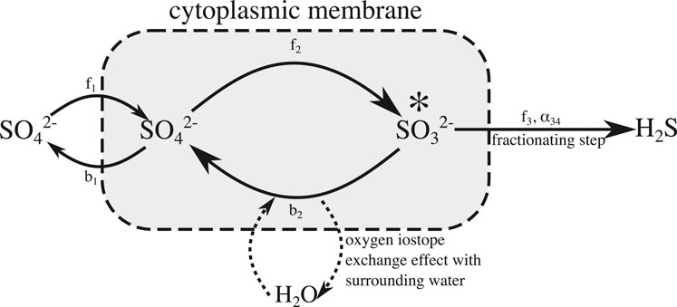
FIGURE 1. Simplified sulfate reduction mechanism used in our model. We have combined steps 2, 3, and 4 described in the text into a single internal reduction step. All of the fractionation factors have been combined into a single overall sulfur fractionation factor in the final step, now made irreversible. The rate of oxygen exchange with the ambient water is tied to the reversibility of the single overall reduction step, as detailed in the text body.
We have combined the reduction of sulfate to sulfite via APS into a single, internal, reversible reduction step (Figure 1). We have done this because we are primarily interested in the rate of oxygen isotope exchange with ambient water, relative to the net rate of sulfate reduction as opposed to identifying any specific pathway by which this isotope exchange occurs or how specific steps in the reaction pathway contribute to this effect. Modeling these intermediate steps as a single, reversible step with a forward and backward reaction rate (f2 and b2 respectively, as shown in Figure 1) is sufficient for exploring the effects of transport, broadly defined, as well as changes in reactivity, on the cross plot of δ34S and δ18O in the extracellular sulfate pool. Typical cross plots of δ34S and δ18O of sulfate at steady state for various amounts of intracellular sulfite recycling are shown in in Figure 2. We will demonstrate that these plots rapidly return to these steady state profiles after dynamic perturbation.
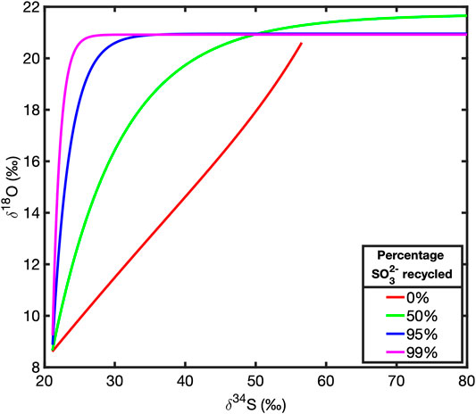
FIGURE 2. Steady state plots of δ34S against δ18O in extracellular sulfate for various percentages of sulfite recycling.
We model the oxygen and sulfur isotope compositions independently, using parallel MSR reaction schemes with rate constants that fractionate each isotope system separately. Each isotope system is subject to the same overall sulfate reduction rate. We now proceed to derive the fractionation factors, for each pair of isotopologues (i = 32, 34 for sulfate, i = 16, 18 for oxygen). For the sulfur isotopologues there will be two reduction rate laws that incorporate the kinetic isotope fractionation of sulfur. For the oxygen isotopologues however, there will be these two reduction rate laws plus an isotope exchange reaction. The former governs the kinetic isotope fractionation of oxygen and the latter the exchange of sulfate-oxygen atoms with the ambient water.
We calculate the sulfur and oxygen isotope fractionation factors by modifying the approaches of Wortmann et al. (2007), Brunner et al. (2012), and Eckert et al. (2011). We assume that the apparent sulfur isotope fractionation is linearly dependent on the amount of sulfite bring recycled within the cell (i.e., how much sulfite is re-oxidized through pathway b2, vs. the amount of sulfite that is reduced to sulfide through pathway f3). We also assume that the cell-reaction pathway is at steady state, as in Eckert et al. (2011) and Brunner et al. (2012). This a good simplifying assumption in this model because the sulfate concentration is greater than the half saturation constant (<1 mM in almost all cases, (Tarpgaard et al., 2011; Tarpgaard et al., 2017)) and thus [SO42-] is not a limiting factor. We parameterize this as a linear relationship by setting the apparent fractionation factor, 34α, to be the sum of two components: one which is constant, fα, and a smaller part, which is the product of a constant β and a parameter Γ, that quantifies the amount of sulfite reflux occurring as a fraction of the overall flux into the branch point marked (*) in Figure 1. When Γ = 0, there is no reflux, when Γ = 1, there is no sulfide production and all the sulfite flux is through the pathway b2. This is expressed in Eq. 1 as suggested by Rees (1973):
Here β determines the maximum change in the apparent sulfur isotope fractionation due to recycling when the mechanism is at steady state. We link this parameter Γ to the rates of the reactions b2 and f2 through the Eq. 2, given that the reaction f3 is irreversible and thus the fraction of sulfite being recycled must be the ratio of b2 to f2. Because Γ is bounded between 0 and 1, we can parameterize the relationship between b2 and f2 in terms of a single parameter, r, which is greater zero. We note that this a purely a mathematical observation and we are not yet assigning any physical meaning to this parameter r.
We assume that the intracellular metabolism is in steady state. At steady state, the difference between the forward and backwards reaction fluxes at each step in the mechanism (Figure 1) must be equal to each other and equal to the total rate of MSR:
Substituting Eq. 2 into Eq. 3 to eliminate f2 we arrive at Eq. 4 which shows that the sulfite reoxidation flux is directly proportional to the overall rate of MSR, Rt. We thus term the parameter r the “recycling factor” because it is the constant of proportionality that determines the amount of sulfite recycling occurring for a given overall MSR rate.
This allows us to rephrase Eq. 1:
Thus, when approximately all of the intermediate valence state sulfur species are recycled, then the isotope fractionation takes on its minimum value, determined by fα. In this study we take fα = 0.975 and β = 0.05 (Rees, 1973; Aller and Blair, 1996; Aharon and Fu, 2000; Aharon and Fu, 2003; Aller et al., 2010; Stam et al., 2011; Antler et al., 2013). So, when return of intermediate valence state sulfur species, or “recycling” approaches 100%, the apparent sulfur isotope fractionation factor approaches 0.925 or an isotope fractionation of −75‰, which we take as the thermodynamic maximum (Brunner et al., 2005; Leavitt et al., 2013; Wing and Halevy, 2014). When there is no recycling, the apparent isotope fractionation of sulfur is −25%.
For oxygen isotope fractionation we determine the value of 18α by taking the kinetic oxygen isotope fractionation (ϵ18 below) to be 25% of the sulfur isotope fractionation (fα) (Aller and Blair, 1996; Aller et al., 2010; Antler et al., 2013).
We have assumed that the kinetic oxygen isotope fractionation factor is not influenced by the fraction of intracellular recycling.
The boundary and initial conditions of the individual sulfate and oxygen isotopologues have been calculated using the isotopic compositions of seawater. A full list of model parameters and their values is given in Table 1.

TABLE 1. A list of model parameters and values. In the cases where the parameter has a dependence on the value of r, we have used r = 14 as a suitable intermediate value that has been suggested to exist in natural environments (Horner and Connick, 2003; Wortmann et al., 2007; Müller, 2013; Wankel et al., 2014).
Reactions Scheme
In implementing our model system in CrunchTope, we explicitly model the concentration of each individual isotopologue within the sediment. We then applied various reactions subject to the available rate laws in CrunchTope. Sulfate reduction was implemented as an irreversible, aqueous reaction with a first order rate dependence on the concentration of the sulfate isotopologue being reduced. We have eschewed a Monod rate equation scheme in favor of a simple first order rate equation because we draw our major conclusions from system behavior at early times, with high sulfate concentrations, and the Monod formulation is equivalent to a first order concentration dependence in that scenario. The kinetic isotope fractionation of the isotopologues was introduced by differing the rate constants for each reduction rate law. The stoichiometry of the reaction is implemented in the model as:
There are four of these irreversible chemical reactions (Eq. 8) in the scheme, one for each of the four isotopologues of sulfate modeled (32SO4, 34SO4, S16O4, and S18O4). Note we do not differentiate among the location of substitution in the case of the oxygen isotopes, we simply assume either no substitution or a single substitution of 16O for 18O. We have chosen to use formaldehyde as the electron donor. This is an arbitrary choice and the concentration is supplied such that the electron donor does not become limiting to the overall rate of the reaction. Thus, the only dependency we explicitly specify is a first-order dependence on sulfate concentration. All of the other species are in excess during the reaction and do not inhibit or enable the reaction in any way; they are included only to satisfy the reaction stoichiometry and the underlying mass balance requirements of the CrunchTope software. The resulting rate law is:
In Eq. 9Ri is the rate of reduction for the sulfate isotopologue, ki is the rate constant, and [SO4]i is the concentration of the sulfate isotopologue in question (i = 16, 18 for the oxygen isotopologues and i = 32, 34 for the sulfur isotopologues).
The oxygen isotope exchange with water was implemented using a single transition state theory (TST) rate law. Instead of explicitly calculating the rates at which different oxygen isotopologues of sulfate are added to and removed from the extracellular sulfate pool as suggested in previous work (Wortmann et al., 2007), we instead explicitly model the oxygen isotope composition of the water. We then allow the oxygen isotopologues to interact with this large ambient water reservoir through the TST rate law, with an equilibrium constant of one. This reaction stoichiometry is given by:
and the resulting rate law is:
In Eq. 11, Rex is the rate of isotope exchange occurring, as specified in the chemical reaction in Eq. 10, while Q is the ion-activity product for the species involved, kex is the rate constant for the exchange of oxygen atoms between the sulfate and ambient water, a parameter we control. We recall that the equilibrium constant, keq = 1. Later, we will demonstrate that we can use the value of Rex, in conjuction with the Wortmann formulation for modeling this isotope exchange (Wortmann et al., 2007) to calculate the value of the recycling parameter, r, as a function of the model input parameters. We note that in Eq. 10, [S18O4] does not indicate a sulfate molecule with four 18O attached, which would be exceedingly rare in nature. It is simply a way of keeping track of the oxygen isotope composition of the sulfate pool as a whole.
We have included a single concentration dependence on the species involved because we want the percentage of intracellular sulfite recycled to be constant (since this is one of the major controls on the SALP (Aller and Blair, 1996; Aller et al., 2010; Antler et al., 2013)), rather than the rate of isotope exchange. This means that the isotope exchange reaction rate needs to be coupled to the rate of sulfate reduction by a constant factor. The easiest way to do this is to introduce a concentration dependance on the major oxygen isotopologue of sulfate (since CrunchTope currently does not allow for concentration dependence on the sum of isotopologues). This approximation works because the major isotope (16O) is approximately 500 times more abundant than the rare isotope (18O). The isotope composition dependence enters through the Q term; the ion activity product which is, in this case:
Because the reservoir of water molecules is so much larger (∼2000 times) than the amount of sulfate in the system, Eqs 11 and 12 suggest that the sulfate oxygen isotope composition is driven to the sulfite-water oxygen isotope equilibrium.
Modeling Sulfur and Oxygen Isotope Fractionation
With the reaction scheme detailed in Eqs 8–11 for the isotopologues i, we need to formulate a set of rate constants, ki, to determine the overall rate of MSR and to incorporate the calculated isotopic fractionations.
We can derive the rate constants for each sulfur isotopologue of sulfate by choosing a time scale for our sulfate reduction reaction. We do this by choosing a maximum rate at which the reaction can proceed. This will be the same for both pairs (32S, and 34S, 16O, and 18O) to ensure that the overall sulfate concentration of each isotope system evolves in the same way. We will term this quantity Rmax and it will represent the rate of sulfate reduction when the total sulfate concentration is 1 M, with the isotopologues assumed to be in their natural (boundary condition) abundances. We set Rmax = 0.00002 mM h−1 and assume that the maximum potential rate of reduction remains constant with depth and time. Considering the rate laws for each isotopologue, shown in Eq. 9, we get the form for Rmax in Eq. 13, given the concentration constraint shown in Eq. 14:
The concentrations [SO4]rare-max and [SO4]common-max are in such a ratio so as to reflect the natural isotopic composition of seawater:
The parameters krare and kcommon represent the rate constants for the rare and common isotopologue in each pair of isotopologues. We now derive pairs of rate constants that incorporate our desired isotope fractionation factors for each pair of isotopologues. Starting from the definition of the isotope fractionation factor given by Rees (1973):
In Eqs. 15–20, α can refer to either 18α or 34α and ξ can refer to either ξS or ξO as is appropriate for either the sulfur or oxygen isotopologue pair.
We then recall Eq. 9 for the rate laws determining Ri and substitute into Eq. 14 which gives:
Combining Eqs. 13-15 or 16 as appropriate allows us to calculate k for each isotopologue, as shown in Eqs 19 and 20. Calculated values of k are shown in Table 3.
Parameterizing the Oxygen Exchange Reaction
The exchange of oxygen isotopes with the ambient water is modeled using a TST reaction, with a rate law given in Eq. 11. The rate law dependencies ensure that the fraction of sulfite being recycled (Γ) is uniform throughout the column.
To relate the rate constant kex to Γ, we consider the rate laws derived by Wortmann et al. (2007). This gives us two separate reaction terms, one for each oxygen isotopologue of sulfate, which we will label ρ16 and ρ18 for the rate of exchange of [S16O4] and [S18O4] with the ambient water, respectively (see Wortmann et al., 2007 for the full mathematical derivation):
It is important to note that the exchange of oxygen atoms with the ambient water cannot change the total amount of sulfate in the system (Wortmann et al., 2007), an assumption that is encapsulated in the reaction scheme shown in Eq. 8:
In Eqs 21 and 22, [SO4] refers to the total sulfate concentration, Rvsmow refers to the Vienna Standard Mean Ocean Water isotopic standard, and b2 is the back-reaction rate shown in Figure 1. The term δout describes the extent to which sulfate that has exchanged oxygen atoms with water inside the cell. Mathematically, this δout term drives the δ18OSO4 to reflect that of isotope exchange with water:
In Eq. 24, δin is the isotopic composition of the sulfate, q parameterizes the extent of isotope exchange taking place, δH2O is the oxygen isotopic composition of the ambient water, and ϵ is an enrichment factor, relating to the equilibrium oxygen isotope effect associated with isotope equilibrium between intermediate valence state sulfur species and water (Horner and Connick, 2003; Wortmann et al., 2007; Brunner et al., 2012; Müller, 2013; Wankel et al., 2014).
Much effort has been made to determine the precise value of ϵ (Betts and Voss, 1970; Horner and Connick, 1986; Horner and Connick, 2003; Zeebe, 2010; Brunner et al., 2012; Müller, 2013; Wankel et al., 2014). For our purposes, the precise value does not matter, as mathematically (or how we have implemented this in the model) it only serves to modify the effective value of δH2O. We choose ϵ = 0 and incorporate any fixed oxygen isotope fractionation associated with isotope exchange with water (which does not vary with space or time or reaction progress) into the value of δH2O, which is explicitly modeled in CrunchTope.
To simplify matters, we take q = 0, reducing Eq. 24 to:
We can now equate Eqs 11 and 22 (one could also use Eqs 21, which provides the same result since ρ16 = -ρ18) to get b2 in terms of the isotope ratio of water, ξambient, the oxygen equilibration rate constant, kex, and the concentrations of the oxygen isotopologues of sulfate. We define ξ in Eq. 26:
Which allows us to express b2 as:
We can then link the isotope exchange reaction flux to the overall rate of sulfate reduction by approximating k18 = k16 which a good approximation in this case (the true difference between the two parameters produces a kinetic fractionation of ∼6‰), shown in Eq. 28. We stress that this approximation in no way implies that we are omitting isotopically fractionating effects in the CrunchTope model. This approximation is merely a mathematical approximation that allows us to determine r for a given set of input parameters.
Substituting Eqs 27 and 29 into Eq. 2, we get an expression for the recycling factor r, in terms of the input parameters for the system, given in Eq. 30:
We will present results for two values of r: r = 0 and r = 14, which correspond to recycling fractions of Γ = 0 and Γ = 0.933. In the former case, there is no exchange of oxygen isotopes with ambient water and the latter case is the amount of intracellular recycling previously suggested to explain pore fluid δ18OSO4 from a site off the coast of Australia (Wortmann et al., 2007).
Model Geometry and Environmental Parameters
Other Model Parameters
We calculate the molecular diffusion of sulfate in seawater, D0 from Schulz (2000).
In Eq. 31, T is the temperature given in degrees Celsius. We take T = 14 °C in this study. We use the same value of D0 for each isotope since the error introduced by this assumption only generates a negligible overestimate of the true isotope fractionation factors in this context, as previously demonstrated by Wortmann and Chernyavsky (2011).
We will initially assume there is no advection and later we will rerun all of the test cases with advection to see how it affects the SALP.
The mesh is made up of a 1D domain with 1,000 nodes equally spaced, each 0.4 cm, giving a sedimentary column of 4 m. The time stepping is handled dynamically by CrunchTope but is limited to a maximum of 1 year per iteration.
Model Test Cases
We model four different test cases (hereafter referred to as Cases 1, 2, 3, and 4—Table 2) as mentioned in the introduction. The boundary conditions are such that the concentrations of the different sulfate isotopologues are fixed at the top of the column, and the concentration gradient of all the species at the bottom of the column is zero. In each case, the whole system evolves to steady state, where we have defined steady state to be reached when the root mean square, over the whole column, of the difference in total concentration of sulfate between a profile at time t and a profile at a time approximately double t is less than 0.000001 mM:
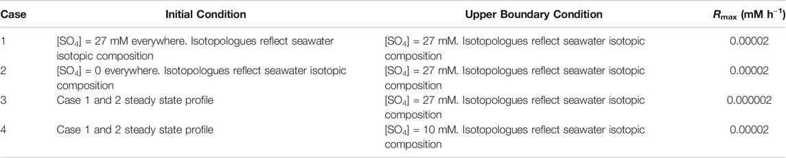
TABLE 2. A list of test cases and their boundary conditions. All cases have the same lower boundary condition of a concentration gradient of zero for all species.
In Eq. 32, [SO4]n(t) refers to the total sulfate concentration at a node n, at a time t and κ is the limit below which the model is deemed to have reached steady state. This value of κ implies that the maximum difference in total concentration between our steady state and a profile that is approximately twice as old at the same node is on the order of 0.01 mM, which is a concentration difference of less than what is analytically resolvable (Kolmert et al., 2000).
This is particularly relevant to Cases 1 and 2, which are designed to investigate the differences in cross plot equilibration behavior when approaching steady state from initial conditions of uniformly high or low concentrations of sulfate.
Case 1
In this case the sulfate concentrations in the sedimentary pore fluids are initially uniform, with concentrations and isotopic composition of pore fluid sulfate the same as seawater. We then initiate MSR throughout the sediment column and allow the system to evolve to steady state. An example of a natural system with a uniform sulfate concentration profile might be a monomictic lake such as Lake Kinneret in Israel or Lake Fukami-Ike, Japan which experience seasonal onset of MSR (Hadas and Pinkas, 1995; Nakagawa et al., 2012; Knossow et al., 2015). Another type of system that can be approximated to first order by the conditions in Case 1 are physically disturbed systems subject to rapid deposition and erosion, like sediments the Amazon Delta. In particular, the mobile suboxic layer described by Aller et al. (2010) that exists in the Amazon Delta and is in part characterized by uniform sulfate concentrations over its profile that are close to that of seawater. Reported increases in δ18OSO4 with no net change in δ34S are congruent with high percentage sulfite recycling and low overall rates of MSR.
Case 2
In Case 2, the sediment is initially without any sulfate in its pore fluid, as for the sediments in a freshwater lake. Then sulfate is added at the top of the sediment column at the concentration and isotopic composition of seawater, similar to what would occur during a marine transgression. The sedimentary porefluids then evolve to steady state, with sulfate supplied from above diffusing into the sediment and undergoing MSR within the sediment.
Case 3
The initial state of the sediment column in this case is the steady-state profile reached in Case 1 and Case 2. In this case, the rate constants, ki, describing the MSR reaction are reduced by a factor of 10. The sedimentary porefluids then evolve with the modified Rt until a new steady state is reached. This perturbation is characteristic of systems in which there has been a step change in the rate of MSR, such as that suggested to occurring over short distances in Lake Van, eastern Turkey (Hadas and Pinkas, 1995; Nakagawa et al., 2012; Knossow et al., 2015) or during seasonal changes in MSR in marginal marine sediments and playa lakes.
Case 4
Similar to Case 3, the initial conditions in the sediment in this case is the steady-state profile from Case 1 and Case 2. The perturbation in this case decreases the concentration of sulfate at the top of the column from 27 to 10 mM, although still with the isotope composition of seawater. The sedimentary pore fluids are then allowed to evolve with the modified boundary conditions. This could be analogous to a restricted freshwater basin which experiences episodic marine influxes, such as the Songliao basin in north-eastern China (Cao et al., 2016).
Results and Discussion
Cross Plot Equilibration
The sulfate pore fluid concentration profiles approach a new steady state as predicted in each of the four test cases (Figure 3). Our test case here is a 4 m sediment column, and we present the total time taken to reach steady state and when the system is 90% of the way to steady state for each perturbation case (Table 3). The time taken to reach steady state is the same regardless of how much recycling is taking place because the exchange of oxygen atoms with ambient water does not impact the concentration of sulfate.
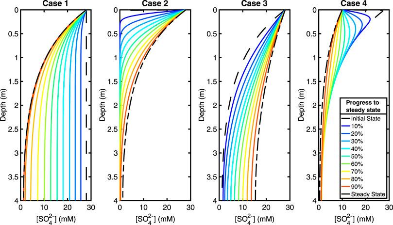
FIGURE 3. Plots showing the evolution of the sulfate concentration with time during the approach to steady state. From left to right, test Cases 1, 2, 3, and 4. Increasing from early to late times as a percentage of the total time to steady state, going from blue (early) to red (late). See legend. See Table 3 for total steady state equilibration times. Equilibration times and concentration profile behaviors are independent of recycling.

TABLE 3. The number of years taken for the system to reach steady state in each case, for a sediment column of 4 m. We note that this is the same regardless of the amount of recycling taking place because the exchange reaction does not affect sulfate concentrations.
The time taken to reach a profile that has a 10% root mean square difference with the final steady state profile (i.e., 90% progress to steady state) is about six to eight times less than the total equilibration time (see Table 3). Thus, the vast majority of adjustment to the imposed perturbation occurs in the earliest stages of the approach to the new steady state.
Figure 4 shows the evolution of the cross plot of δ34S vs. δ18OSO4, for each test case, with and without intracellular recycling occurring. When r = 0 (i.e., no recycling is occurring) we see that the cross plot remains the same for all cases at all times. This is because there is no sulfite-water equilibrium (r = 0) and so the δ34S and δ18OSO4 evolve mathematically via the same differential equation and as the model does not prescribe any explicit differentiation by transport, the depth plots of δ34S and δ18OSO4 behave in the same way. This preserves their ratio at all times and at all depths, mapping the SALP onto a straight line.
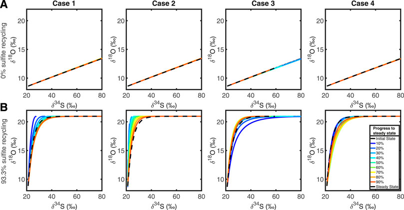
FIGURE 4. Top row, (A): plots showing the evolution of the δ34S and δ18O cross plots through time, in each test case, for r = 0, which corresponds to 0% of the sulfite is being recycled. Bottom row, (B): in order, test cases 1, 2, 3, and 4 when 93.3% of sulfite is being recycled.
When the recycling parameter is non-zero, (in Figure 4A, r = 0) then there is intracellular recycling and oxygen isotopes are exchanged with water through various (unspecified) intermediates. The cross plot shows both the apparent linear phase and the equilibration phase, with an asymptote as δ34S continues to increase as the sulfate pool undergoes MSR, while δ18OSO4 remains constant once oxygen isotopic equilibrium with water is reached (Fritz et al., 1989; Aller and Blair, 1996; Aller et al., 2010; Antler et al., 2013; Antler et al., 2017; Bertran et al., 2020).
Our model reproduces the anticipated behavior of the cross plot of δ34S vs. δ18OSO4; with SALP steeper with increased intracellular recycling (the slope in Figures 4A vs. 4B), as previously observed (Aller and Blair, 1996; Aller et al., 2010; Antler et al., 2013; Antler et al., 2017). When more recycling occurs, more exchange of oxygen isotopes with water occurs per unit time (Figure 2). We also note that different perturbations cause SALP to be both over or underestimated during the initial response to the perturbation; when sulfate reduction is imposed on a sediment column (Case 1 and 2), SALP is initially steeper than it will be at steady state. When the rate of MSR decreases, however (Case 3), SALP is initially shallower than it will be at steady state. Our results suggest that perturbations to steady state dissipate within the first half of the run time in each case.
Investigating Slope of the Apparent Linear Phase
One goal of this work is to understand the potential error in measuring SALP in natural pore fluids due to non-steady state effects. We now present the behavior of the SALP during the approach to steady state in an effort to quantify this potential error. Figure 5 shows how quickly the δ34S and δ18OSO4, sulfate concentrations and SALP reach new steady state after the perturbation in Case 1. Figure 5 suggests that the gradient of the δ18OSO4 adjusts rapidly to a perturbation, and that sulfate concentrations adjustment is much slower. The δ34SSO4 depth profile equilibrates slower than the δ18OSO4 depth profile but will be always be faster than the [SO42-] depth profile. This is because the hypothetical diffusion constant required for the sulfate concentration to equilibrate at a similar rate to δ34SSO4 is unrealistic, even if we discount potential second order effects that increasing the diffusion constant may have to speed up isotope composition equilibration. The adjustment to SALP after a perturbation will be rate-limited by the isotopologue that adjusts more slowly to the perturbation, our model suggests that for Case 1 (and for all other tested cases) this is δ34SSO4. This is why SALP approaches a new steady state over the same timescale as δ34SSO4.
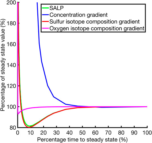
FIGURE 5. Plot of the slope of the apparent linear phase for the δ34S and δ18O cross plot and other quantities plotted against the percentage progress to steady state through time. Case 1, r = 14.
This reflects the underlying principle that the processes at work in this system mean that the gradients of interest equilibrate in either an overdamped or underdamped way. The results of the model suggest δ34S and δ18O in the porefluid depth profile gradients equilibrate more rapidly, with the key feature of their equilibration being their overdamped (over-shoot of the final value) behavior. This bounds their values to within the vicinity of the steady state result from very early times. In contrast, the concentration depth profile gradient is underdamped (monotonically approaches the final value) in its approach to steady state and as a result does not exhibit the overshoot behavior that confines the δ34S and δ18O depth profile gradients close to the steady state value. In particular δ18OSO4 will either evolve under the same equations as δ34SSO4, in the case when r = 0, or more rapidly in cases where r ≠ 0 (as seen in Figure 5) because of the equilibration of sulfite with ambient water. This hierarchy of equilibration behaviors means that SALP equilibration is primarily determined by the δ34SSO4 isotope composition gradient behavior, and since both the δ18OSO4 and δ34SSO4 gradients are overdamped, the SALP is close to the steady state value from early times and thus resistant to dynamic perturbations.
We note that the timescale over which SALP might be incorrect due to a perturbation is vanishingly small in most natural environments (Figure 6A). For example, in a lake we’d expect SALP to be out of equilibrium for a few hours after some hypothetical perturbation, while in marginal marine sedimentary pore fluids up to a month; it is unlikely we would capture this transience in sampling (although one may be unlucky). We further quantify the potential error in measured SALP as a function of the percentage sulfite recycling occurring (Figure 6B). We note that the potential error in the measurement of SALP increases as the percentage recycling increases. We suggest that this is because of the variable behavior of δ18OSO4 as the percentage of recycling increases. The error bars were generated by considering the minimum of the SALP during its evolution to steady state (see Figure 5 for an example of this minimum).
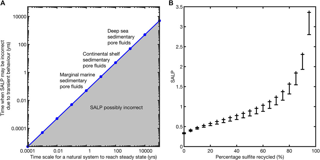
FIGURE 6. Left,(A); a schematic plot showing the time scales over which the measurement of the SALP may be unreliable. Our modeling suggests that this is approximately the first 5% of the total time to steady state and that this effect is scale independent. Right,(B); a plot of the SALP and the maximum error in its measurement as a function of the percentage recycling taking place. The error bars represent the maximum deviation of the SALP from its steady state value during its approach to steady state, ignoring the first 5% of equilibration time in which the SALP is many orders of magnitude wrong, see equilibration behavior in Figure 5.
We consider our model results to three previously published sites, a river estuary, a shallow marine site, and a deep marine site (Antler et al., 2013). The published SALP of these three sites (1.4, 0.99, and 0.35 respectively), along with the depth over which MSR occurs (0.25, 2.5, and 200 m respectively), can be used to determine the timescale over which the SALP would record a perturbation to steady state. In the estuarine site, large perturbations would be visible for less than half a year. Similarly, these large perturbations are suggested to dissipate in the shallow and deep marine sites in approximately 13 and 83,000 years respectively. Deep marine sedimentary pore fluids are assumed to be in steady state and not subject to perturbations similar to the case studies we have employed.
An interesting intermediate case is presented in the work of Contreras et al. (2013) which glacial-interglacial periodicity in sealevel driving movement in the sulfate pore fluid profiles on the scale of tens of meters. While this particular type of perturbation does not correspond directly to any of our test cases, it is most closely identifiable with Case 4 under which the sulfate concentration boundary condition is varied after reaching steady state. The model proposed by Contreras suggests an equilibration time of ∼100 ka for the pore fluid sulfate concentrations. We would therefore predict that perturbations to SALP would be negligible after the first ∼5,000 years after the change in sealevel but we acknowledge that the movement of the sulfate-methane transition zone under this perturbation has not been accounted for in our model. Integration of isotope enabled anaerobic oxidation of methane and methanogenesis into our analysis of non-steady state effects on the SALP could be a potentially insightful area of future study.
We suggest that it is extremely unlikely that any natural samples would record SALP analytically resolvable to be out of steady state; in deep-marine sediments there is not a process to push the system so far out of steady state, while in shallow marine, marginal marine, and terrestrial systems the response time is fast enough that we would not capture it. This means that the maximum error in the SALP is associated with recycling (Figure 6B).
The Effect of Advection
We can determine whether advection is important in any porous media by evaluating the Péclet number, Pe:
The terms w and v are the rates of advection due to flow and sediment burial respectively. The parameter D0 is the coefficient of molecular diffusion as given in Eq. 31. The length L is the length scale over which the equilibration of the system occurs, in this case we take L = 1 m. Using a constant advective flux of v = 50 m Ma−1 (toward the upper limit of what has been observed in deep sea environments) we get Pe = 2.0756 × 10⁻³. We therefore expect advection to have a negligible effect on these kinds of system in nature, and this borne out in our modeling.
To test the effect of advection, we applied two artificially large advective fluxes to t the system, v = 24.09 km Ma−1 (Pe = 1) and v = 2,409 km Ma−1 (Pe = 100). The results from the first case are shown in Figure 7. Figure 7A shows the normal behavior with no advective flux and Figure 7B shows the evolution of the cross plots when Pe = 1. We see that the SALP cross plots are largely unchanged, with the plots behaving in the same manner, with a slight increase in the timescale for isotopic equilibration.
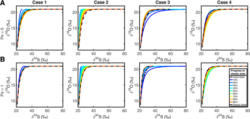
FIGURE 7. Top row, (A): Plots of δ34S against δ18O in extracellular sulfate without an advective flux (Pe = 0). Bottom row, (B): Cross plots of δ34S against δ18O with an advective flux of 24.09 km Ma−1 (Pe = 1), in each test case. Comparing the top and bottom rows demonstrates that advection has no significant effect on the nature of the isotope cross plots.
The latter case (Pe = 100, not shown) shows that the entire δ18OSO4 – δ34SSO4 cross plot is mapped to an almost vertical straight line at δ34SSO4 = ∼ 20‰ (the seawater value), with the usual range of δ18OSO4 (8–22‰). We interpret this as the continual flushing with the system with seawater sulfate before meaningful MSR can occur, while oxygen isotope exchange with ambient water is sufficiently rapid as to still be seen in the pore fluid sulfate. We predict that with sufficiently rapid advective flux that this may no longer be possible, effectively mapping the δ34S and δ18O cross plot of sulfate to a point at seawater composition. So, with sufficiently high advective fluxes, it is possible to erase the SALP value, but these fluxes are so unrealistic for natural systems we consider the result to be unimportant. We conclude that we can ignore the effects of advection in measuring and interpreting SALP.
Summary
We have presented the results of a 1D isotope-enabled reactive transport model to demonstrate the effects of transport and non-steady state behavior on the sulfur and oxygen isotopic compositions in sediments undergoing MSR. In particular we explored the effects of these phenomena on the δ34S and δ18O cross plot for extracellular sulfate and assessed its utility under conditions of variable transport and non-steady state dynamics.
The steady state that the system approaches is unaffected by the choice of boundary conditions or direction of approach, demonstrated in test Cases 1 and 2. However, the time scale over which the system reaches steady state was determined in part by the choice of initial conditions because this dictates whether diffusion or reaction acts as the primary driver toward steady state. Our results suggested that the system will approach 90% stability in approximately half the time between perturbation and the new steady state.
Cases 3 and 4 shows that perturbations within the sediment column have a minimal effect on the δ34S vs. δ18O cross plot, and any effect rapidly decays, relative the overall equilibration time scale. The SALP rapidly reaches a new steady state after a perturbation, after approximately 5% of the total time. This appears to be a length-scale-independent behavior, provided that reaction rates are scaled with the column length. Ignoring this initial time period in which measurements of the SALP may be incorrect, we have shown that the error in the SALP grows with the amount of recycling taking place in the system, and that this error grows in the same way as the equilibrium value of the SALP itself.
Applying these principles to three previously published profiles in three different environments (estuarine, shallow marine, and deep marine) leads us to conclude that the measurements made of the SALP in those studies can be interpreted in terms of microbial metabolism and not in terms of changes in transport dynamics.
We conclude that perturbations due to transport and non-steady state dynamics on the plot of δ34S against δ18O in extracellular sulfate are negligible. Although the δ18O depth profile gradient appears to equilibrate more rapidly than the SALP does, due to the forcing effect of the exchange of sulfate oxygen with the surrounding water, the SALP remains a good tool for investigating MSR rates because it is minimally affected by advective transport. Perturbation effects are non-existent when there is no pore water oxygen isotope exchange occurring and increase with the amount of recycling. Thus, in sedimentary environments the SALP can be interpreted as a function of microbial metabolism, not in terms of environmental perturbations.
Data Availability Statement
All datasets presented in this study can be found in online repositories. The names of the repository/repositories and accession number(s) can be found below: https://github.com/a-fotherby/crunchtope-nss-crossplot-model.
Author Contributions
GA, AT, XS contributed to conception and design of the study. AF designed and implemented the model and analyzed the results. HB, JD advised the implementation of the model. AF wrote the first draft of the manuscript. AF, AT, GA wrote sections of the manuscript. All authors contributed to manuscript revision, read, and approved the submitted version.
Funding
The work was supported by ERC 307582 StG (CARBON-SINK) to AT, NERC NE/R013519/1 to HB, ISF (2361/19) to GA, and by a NERC ESS DTP Research Experience Placement to AF.
Conflict of Interest
The authors declare that the research was conducted in the absence of any commercial or financial relationships that could be construed as a potential conflict of interest.
Supplementary Material
The Supplementary Material for this article can be found online at: https://www.frontiersin.org/articles/10.3389/feart.2020.587085/full#supplementary-material.
References
Aharon, P., and Fu, B. (2000). Microbial sulfate reduction rates and sulfur and oxygen isotope fractionations at oil and gas seeps in deepwater Gulf of Mexico. Geochem. Cosmochim. Acta. 64, 233–246. doi:10.1016/S0016-7037(99)00292-6
Aharon, P., and Fu, B. (2003). Sulfur and oxygen isotopes of coeval sulfate-sulfide in pore fluids of cold seep sediments with sharp redox gradients. Chem. Geol. 195, 201–218. doi:10.1016/S0009-2541(02)00395-9
Akagi, J. M. (1995). “Respiratory sulfate reduction,” in sulfate-reducing bacteria biotechnology handbooks. Editor L. L. Barton (Boston, MA: Springer US), 89–111.
Algeo, T. J., Luo, G. M., Song, H. Y., Lyons, T. W., and Canfield, D. E. (2015). Reconstruction of secular variation in seawater sulfate concentrations. Biogeosciences 12, 2131–2151. doi:10.5194/bg-12-2131-2015
Aller, R. C., and Blair, N. E. (1996). Sulfur diagenesis and burial on the Amazon shelf: major control by physical sedimentation processes. Geo Mar. Lett. 16, 3–10. doi:10.1007/bf01218830
Aller, R. C., Madrid, V., Chistoserdov, A., Aller, J. Y., and Heilbrun, C. (2010). Unsteady diagenetic processes and sulfur biogeochemistry in tropical deltaic muds: implications for oceanic isotope cycles and the sedimentary record. Geochem. Cosmochim. Acta. 74, 4671–4692. doi:10.1016/j.gca.2010.05.008
Antler, G., and Pellerin, A. (2018). A critical look at the combined use of sulfur and oxygen isotopes to study microbial metabolisms in methane-rich environments. Front. Microbiol. 9, 519. doi:10.3389/fmicb.2018.00519
Antler, G., Turchyn, A. V., Herut, B., Davies, A., Rennie, V. C. F., and Sivan, O. (2014). Sulfur and oxygen isotope tracing of sulfate driven anaerobic methane oxidation in estuarine sediments. Estuar. Coast Shelf Sci. 142, 4–11. doi:10.1016/j.ecss.2014.03.001
Antler, G., Turchyn, A. V., Herut, B., and Sivan, O. (2015). A unique isotopic fingerprint of sulfate-driven anaerobic oxidation of methane. Geology 43, 619–622. doi:10.1130/g36688.1
Antler, G., Turchyn, A. V., Ono, S., Sivan, O., and Bosak, T. (2017). Combined 34S, 33S and 18O isotope fractionations record different intracellular steps of microbial sulfate reduction. Geochem. Cosmochim. Acta. 203, 364–380. doi:10.1016/j.gca.2017.01.015
Antler, G., Turchyn, A. V., Rennie, V., Herut, B., and Sivan, O. (2013). Coupled sulfur and oxygen isotope insight into bacterial sulfate reduction in the natural environment. Geochem. Cosmochim. Acta. 118, 98–117. doi:10.1016/j.gca.2013.05.005
Balci, N., Shanks, W. C., Mayer, B., and Mandernack, K. W. (2007). Oxygen and sulfur isotope systematics of sulfate produced by bacterial and abiotic oxidation of pyrite. Geochem. Cosmochim. Acta. 71, 3796–3811. doi:10.1016/j.gca.2007.04.017
Böttcher, M. E., Bernasconi, S. M., and Brumsack, H.-J. (1999). Carbon, sulfur, and oxygen isotope geochemistry of interstitial waters from the western Mediterranien. Proc. Ocean Drill. Prog. Sci. Results. 161, 413–421.
Böttcher, M. E., Brumsack, H.-J., and De Lange, G. J. (1998). “Sulfate reduction and related stable isotope (34S, 18O) variations in interstitial waters from the Eastern Mediterranean,” in Proceedings-ocean drilling program scientific results. Editors A. H. F. Robertson, K.-C. Emeis, C. Richter, and A. Camerlenghi, (Alexandria, VA: National Science Foundation), 365–376.
Böttcher, M. E., Hespenheide, B., Llobet-Brossa, E., Beardsley, C., Larsen, O., Schramm, A., et al. (2000). The biogeochemistry, stable isotope geochemistry, and microbial community structure of a temperate intertidal mudflat: an integrated study. Continent. Shelf Res. 20, 1749–1769. doi:10.1016/s0278-4343(00)00046-7
Böttcher, M. E., and Thamdrup, B. (2001). Anaerobic sulfide oxidation and stable isotope fractionation associated with bacterial sulfur disproportionation in the presence of MnO2. Geochem. Cosmochim. Acta. 65, 1573–1581. doi:10.1016/s0016-7037(00)00622-0
Böttcher, M. E., Thamdrup, B., Gehre, M., and Theune, A. (2005). 34S/32S and 18O/16O fractionation during sulfur disproportionation by Desulfobulbus propionicus. Geomicrobiol. J. 22, 219–226. doi:10.1080/01490450590947751
Böttcher, M. E., Thamdrup, B., and Vennemann, T. W. (2001). Oxygen and sulfur isotope fractionation during anaerobic bacterial disproportionation of elemental sulfur. Geochem. Cosmochim. Acta. 65, 1601–1609. doi:10.1016/s0016-7037(00)00628-1
Berner, R. A. (1980). Early diagenesis: a theoretical approach. Princeton, NY: Princeton University Press.
Bertran, E., Waldeck, A., Wing, B. A., Halevy, I., Leavitt, W. D., Bradley, A. S., et al. (2020). Oxygen isotope effects during microbial sulfate reduction: applications to sediment cell abundances. ISME J. 14, 1508–1519. doi:10.1038/s41396-020-0618-2
Betts, R. H., and Voss, R. H. (1970). The kinetics of oxygen exchange between the sulfite ion and water. Can. J. Chem. 48, 2035–2041. doi:10.1139/v70-339
Blonder, B., Boyko, V., Turchyn, A. V., Antler, G., Sinichkin, U., Knossow, N., et al. (2017). Impact of aeolian dry deposition of reactive iron minerals on sulfur cycling in sediments of the Gulf of aqaba. Front. Microbiol. 8, 1131. doi:10.3389/fmicb.2017.01131
Bowles, M. W., Mogollón, J. M., Kasten, S., Zabel, M., and Hinrichs, K.-U. (2014). Global rates of marine sulfate reduction and implications for sub-sea-floor metabolic activities. Science 344, 889–891. doi:10.1126/science.1249213
Bradley, A. S., Leavitt, W. D., and Johnston, D. T. (2011). Revisiting the dissimilatory sulfate reduction pathway. Geobiology 9, 446–457. doi:10.1111/j.1472-4669.2011.00292.x
Bradley, A. S., Leavitt, W. D., Schmidt, M., Knoll, A. H., Girguis, P. R., and Johnston, D. T. (2016). Patterns of sulfur isotope fractionation during microbial sulfate reduction. Geobiology 14, 91–101. doi:10.1111/gbi.12149
Bruchert, V. (2004). Physiological and ecological aspects of sulfur isotope fractionation during bacterial sulfate reduction. Spec. Pap.-Geol. Soc. Am. 379, 1–16. doi:10.1130/0-8137-2379-5.1
Brunner, B., Bernasconi, S. M., Kleikemper, J., and Schroth, M. H. (2005). A model for oxygen and sulfur isotope fractionation in sulfate during bacterial sulfate reduction processes. Geochem. Cosmochim. Acta. 69, 4773–4785. doi:10.1016/j.gca.2005.04.017
Brunner, B., Einsiedl, F., Arnold, G. L., Müller, I., Templer, S., and Bernasconi, S. M. (2012). The reversibility of dissimilatory sulphate reduction and the cell-internal multi-step reduction of sulphite to sulphide: insights from the oxygen isotope composition of sulphate. Isot. Environ. Health Stud. 48, 33–54. doi:10.1080/10256016.2011.608128
Brunner, B., Yu, J.-Y., Mielke, R. E., MacAskill, J. A., Madzunkov, S., McGenity, T. J., et al. (2008). Different isotope and chemical patterns of pyrite oxidation related to lag and exponential growth phases of Acidithiobacillus ferrooxidans reveal a microbial growth strategy. Earth Planet Sci. Lett. 270, 63–72. doi:10.1016/j.epsl.2008.03.019
Canfield, D. E. (1998). A new model for Proterozoic ocean chemistry. Nature 396, 450–453. doi:10.1038/24839
Canfield, D. E. (2001). Biogeochemistry of sulfur isotopes. Rev. Mineral. Geochem. 43, 607–636. doi:10.2138/gsrmg.43.1.607
Canfield, D. E., Stewart, F. J., Thamdrup, B., De Brabandere, L., Dalsgaard, T., Delong, E. F., et al. (2010). A cryptic sulfur cycle in oxygen-minimum-zone waters off the Chilean coast. Science 330, 1375–1378. doi:10.1126/science.1196889
Cao, H., Kaufman, A. J., Shan, X., Cui, H., and Zhang, G. (2016). Sulfur isotope constraints on marine transgression in the lacustrine Upper Cretaceous Songliao Basin, northeastern China. Palaeogeogr. Palaeoclimatol. Palaeoecol. 451, 152–163. doi:10.1016/j.palaeo.2016.02.041
Chernyavsky, B. M., and Wortmann, U. G. (2007). REMAP: a reaction transport model for isotope ratio calculations in porous media. Geochem. Geophys. Geosystems. 8, 654–656. doi:10.1029/2006gc001442
Contreras, S., Meister, P., Liu, B., Prieto-Mollar, X., Hinrichs, K.-U., Khalili, A., et al. (2013). Cyclic 100-ka (glacial-interglacial) migration of subseafloor redox zonation on the Peruvian shelf. Proc. Natl. Acad. Sci. 110, 18098–18103. doi:10.1073/pnas.1305981110
Davidson, M. M., Bisher, M. E., Pratt, L. M., Fong, J., Southam, G., Pfiffner, S. M., et al. (2009). Sulfur isotope enrichment during maintenance metabolism in the thermophilic sulfate-reducing bacterium Desulfotomaculum putei. Appl. Environ. Microbiol. 75, 5621–5630. doi:10.1128/aem.02948-08
D’Hondt, S. (2004). Distributions of microbial activities in deep subseafloor sediments. Science 306, 2216–2221. doi:10.1126/science.1101155
Deusner, C., Holler, T., Arnold, G. L., Bernasconi, S. M., Formolo, M. J., and Brunner, B. (2014). Sulfur and oxygen isotope fractionation during sulfate reduction coupled to anaerobic oxidation of methane is dependent on methane concentration. Earth Planet Sci. Lett. 399, 61–73. doi:10.1016/j.epsl.2014.04.047
Donahue, M. A., Werne, J. P., Meile, C., and Lyons, T. W. (2008). Modeling sulfur isotope fractionation and differential diffusion during sulfate reduction in sediments of the Cariaco Basin. Geochem. Cosmochim. Acta. 72, 2287–2297. doi:10.1016/j.gca.2008.02.020
Eckert, T., Brunner, B., Edwards, E. A., and Wortmann, U. G. (2011). Microbially mediated re-oxidation of sulfide during dissimilatory sulfate reduction by Desulfobacter latus. Geochem. Cosmochim. Acta. 75, 3469–3485. doi:10.1016/j.gca.2011.03.034
Egger, M., Riedinger, N., Mogollón, J. M., and Jørgensen, B. B. (2018). Global diffusive fluxes of methane in marine sediments. Nat. Geosci. 11, 421–425. doi:10.1038/s41561-018-0122-8
Farquhar, J., Canfield, D. E., Masterson, A., Bao, H., and Johnston, D. (2008). Sulfur and oxygen isotope study of sulfate reduction in experiments with natural populations from Fællestrand, Denmark. Geochem. Cosmochim. Acta. 72, 2805–2821. doi:10.1016/j.gca.2008.03.013
Farquhar, J., Johnston, D. T., Wing, B. A., Habicht, K. S., Canfield, D. E., Airieau, S., et al. (2003). Multiple sulphur isotopic interpretations of biosynthetic pathways: implications for biological signatures in the sulphur isotope record. Geobiology 1, 27–36. doi:10.1046/j.1472-4669.2003.00007.x
Fitz, R. M., and Cypionka, H. (1990). Formation of thiosulfate and trithionate during sulfite reduction by washed cells of Desulfovibrio desulfuricans. Arch. Microbiol. 154, 400–406. doi:10.1007/BF00276538
Fritz, P., Basharmal, G. M., Drimmie, R. J., Ibsen, J., and Qureshi, R. M. (1989). Oxygen isotope exchange between sulphate and water during bacterial reduction of sulphate. Chem. Geol. Isot. Geosci. 79, 99–105. doi:10.1016/0168-9622(89)90012-2
Garrels, R. M., and Lerman, A. (1984). Coupling of the sedimentary sulfur and carbon cycles; an improved model. Am. J. Sci. 284, 989–1007. doi:10.2475/ajs.284.9.989
Giannetta, M. G., Sanford, R. A., and Druhan, J. L. (2019). A modified Monod rate law for predicting variable S isotope fractionation as a function of sulfate reduction rate. Geochem. Cosmochim. Acta. 258, 174–194. doi:10.1016/j.gca.2019.05.015
Glombitza, C., Stockhecke, M., Schubert, C. J., Vetter, A., and Kallmeyer, J. (2013). Sulfate reduction controlled by organic matter availability in deep sediment cores from the saline, alkaline Lake Van (Eastern Anatolia, Turkey). Front. Microbiol. 4, 209. doi:10.3389/fmicb.2013.00209
Gomes, M. L., and Johnston, D. T. (2017). Oxygen and sulfur isotopes in sulfate in modern euxinic systems with implications for evaluating the extent of euxinia in ancient oceans. Geochem. Cosmochim. Acta. 205, 331–359. doi:10.1016/j.gca.2017.02.020
Habicht, K. S., Salling, L., Thamdrup, B., and Canfield, D. E. (2005). Effect of low sulfate concentrations on lactate oxidation and isotope fractionation during sulfate reduction by archaeoglobus fulgidus strain Z†. Aemilianense 71, 3770–3777. doi:10.1128/aem.71.7.3770-3777.2005
Hadas, O., and Pinkas, R. (1995). Sulphate reduction in the hypolimnion and sediments of Lake Kinneret, Israel. Freshw. Biol. 33, 63–72. doi:10.1111/j.1365-2427.1995.tb00386.x
Heidel, C., and Tichomirowa, M. (2011). The isotopic composition of sulfate from anaerobic and low oxygen pyrite oxidation experiments with ferric iron - new insights into oxidation mechanisms. Chem. Geol. 281, 305–316. doi:10.1016/j.chemgeo.2010.12.017
Hilz, H., and Lipmann, F. (1955). The enzymatic activation of sulfate. Proc. Natl. Acad. Sci. Unit. States Am. 41, 880–890. doi:10.1073/pnas.41.11.880
Horner, D. A., and Connick, R. E. (1986). Equilibrium quotient for the isomerization of bisulfite ion from HSO3- to SO3H-. Inorg. Chem. 25, 2414–2417. doi:10.1021/ic00234a026
Horner, D. A., and Connick, R. E. (2003). Kinetics of oxygen exchange between the two isomers of bisulfite ion, disulfite ion (S2O52-), and water as studied by oxygen-17 nuclear magnetic resonance spectroscopy. Inorg. Chem. 42, 1884–1894. doi:10.1021/ic020692n
Johnston, D. T. (2005). Active microbial sulfur disproportionation in the mesoproterozoic. Science 310, 1477–1479. doi:10.1126/science.1117824
Johnston, D. T., Farquhar, J., and Canfield, D. E. (2007). Sulfur isotope insights into microbial sulfate reduction: when microbes meet models. Geochem. Cosmochim. Acta. 71, 3929–3947. doi:10.1016/j.gca.2007.05.008
Jorgensen, B. B. (1979). A theoretical model of the stable sulfur isotope distribution in marine sediments. Geochem. Cosmochim. Acta. 43, 363–374. doi:10.1016/0016-7037(79)90201-1
Jørgensen, B. B. (1982). Mineralization of organic matter in the sea bed-the role of sulphate reduction. Nature 296, 643–645. doi:10.1038/296643a0
Jørgensen, B. B., Findlay, A. J., and Pellerin, A. (2019). The biogeochemical sulfur cycle of marine sediments. Front. Microbiol. 10, 849.
Kasten, S., and Jørgensen, B. B. (2000). “Sulfate reduction in marine sediments,” inMarine geochemistry. Editors H. D. Schulz, and M. Zabel (Berlin, Heidelberg: Springer), 263–281. doi:10.1007/978-3-662-04242-7_8
Kasten, S., Zabel, M., Heuer, V., and Hensen, C. (2003). “Processes and signals of nonsteady-state diagenesis in deep-sea sediments and their pore waters,” inThe South Atlantic in the late quaternary. Editors G. Wefer, S. Mulitza, and V. Ratmeyer (Berlin, Heidelberg: Springer), 431–459.
King, G. M. (2001). Radiotracer assays (35S) of sulfate reduction rates in marine and freshwater sediments. Methods Microbiol. 30, 489–500. doi:10.1016/s0580-9517(01)30059-4
Knöller, K., Vogt, C., Richnow, H.-H., and Weise, S. M. (2006). Sulfur and oxygen isotope fractionation during benzene, toluene, ethyl benzene, and xylene degradation by sulfate-reducing bacteria. Environ. Sci. Technol. 40, 3879–3885. doi:10.1021/es052325r
Knossow, N., Blonder, B., Eckert, W., Turchyn, A. V., Antler, G., and Kamyshny, A. (2015). Annual sulfur cycle in a warm monomictic lake with sub-millimolar sulfate concentrations. Geochem. Trans. 16, 7. doi:10.1186/s12932-015-0021-5
Kobayashi, K., Tachibana, S., and Ishimoto, M. (1969). Intermediary formation of trithionate in sulfite reduction by a sulfate-reducing bacterium. J. Biochem. (Tokyo) 65, 155–157.
Kohl, I., and Bao, H. (2011). Triple-oxygen-isotope determination of molecular oxygen incorporation in sulfate produced during abiotic pyrite oxidation (pH=2-11). Geochem. Cosmochim. Acta. 75, 1785–1798. doi:10.1016/j.gca.2011.01.003
Kolmert, Å., Wikström, P., and Hallberg, K. B. (2000). A fast and simple turbidimetric method for the determination of sulfate in sulfate-reducing bacterial cultures. J. Microbiol. Methods. 41, 179–184. doi:10.1016/S0167-7012(00)00154-8
Leavitt, W. D., Bradley, A. S., Santos, A. A., Pereira, I. A. C., and Johnston, D. T. (2015). Sulfur isotope effects of dissimilatory sulfite reductase. Front. Microbiol. 6, 1392. doi:10.3389/fmicb.2015.01392
Leavitt, W. D., Halevy, I., Bradley, A. S., and Johnston, D. T. (2013). Influence of sulfate reduction rates on the Phanerozoic sulfur isotope record. Proc. Natl. Acad. Sci. Unit. States Am. 110, 11244–11249. doi:10.1073/pnas.1218874110
Liu, J., Pellerin, A., Antler, G., Kasten, S., Findlay, A. J., Dohrmann, I., et al. (2020). Early diagenesis of iron and sulfur in Bornholm Basin sediments: the role of near-surface pyrite formation. Geochim. Cosmochim. Acta 284, 43–60.
Mangalo, M., Einsiedl, F., Meckenstock, R. U., and Stichler, W. (2008). Influence of the enzyme dissimilatory sulfite reductase on stable isotope fractionation during sulfate reduction. Geochem. Cosmochim. Acta. 72, 1513–1520. doi:10.1016/j.gca.2008.01.006
Mangalo, M., Meckenstock, R. U., Stichler, W., and Einsiedl, F. (2007). Stable isotope fractionation during bacterial sulfate reduction is controlled by reoxidation of intermediates. Geochem. Cosmochim. Acta. 71, 4161–4171. doi:10.1016/j.gca.2007.06.058
Mills, J. V., Antler, G., and Turchyn, A. V. (2016). Geochemical evidence for cryptic sulfur cycling in salt marsh sediments. Earth Planet Sci. Lett. 453, 23–32. doi:10.1016/j.epsl.2016.08.001
Mizutani, Y., and Rafter, T. A. (1969). Bacterial fractionation of oxygen isotopes in the reduction of sulphate and in the oxidation of sulphur. N. Z. J. Sci. 12, 60–68.
Müller, I. A. (2013). The pivotal role of sulfite species in shaping the oxygen isotope composition of sulfate: new insights from a stable isotope perspective. 173.
Nakagawa, M., Ueno, Y., Hattori, S., Umemura, M., Yagi, A., Takai, K., et al. (2012). Seasonal change in microbial sulfur cycling in monomictic Lake Fukami-ike, Japan. Limnol. Oceanogr. 57, 974–988. doi:10.4319/lo.2012.57.4.0974
Niewöhner, C., Hensen, C., Kasten, S., Zabel, M., and Schulz, H. D. (1998). Deep sulfate reduction completely mediated by anaerobic methane oxidation in sediments of the upwelling area off Namibia. Geochem. Cosmochim. Acta. 62, 455–464. doi:10.1016/S0016-7037(98)00055-6
Pasquier, V., Sansjofre, P., Rabineau, M., Revillon, S., Houghton, J., and Fike, D. A. (2017). Pyrite sulfur isotopes reveal glacial−interglacial environmental changes. Proc. Natl. Acad. Sci. U.S.A. 114, 5941–5945. doi:10.1073/pnas.1618245114
Pellerin, A., Antler, G., Marietou, A., Turchyn, A. V., and Jørgensen, B. B. (2020). The effect of temperature on sulfur and oxygen isotope fractionation by sulfate reducing bacteria (Desulfococcus multivorans). FEMS Microbiol. Lett. 367, fnaa061. doi:10.1093/femsle/fnaa061
Pellerin, A., Bui, T. H., Rough, M., Mucci, A., Canfield, D. E., and Wing, B. A. (2015). Mass-dependent sulfur isotope fractionation during reoxidative sulfur cycling: a case study from Mangrove Lake, Bermuda, Geochem. Cosmochim. Acta. 149, 152–164. doi:10.1016/j.gca.2014.11.007
Reeburgh, W. S. (2007). Oceanic methane biogeochemistry. Chem. Rev. 107, 486–513. doi:10.1021/cr050362v
Rees, C. E. (1973). A steady-state model for sulphur isotope fractionation in bacterial reduction processes. Geochem. Cosmochim. Acta. 37, 1141–1162. doi:10.1016/0016-7037(73)90052-5
Rees, C. E., Jenkins, W. J., and Monster, J. (1978). The sulphur isotopic composition of ocean water sulphate. Geochem. Cosmochim. Acta. 42, 377–381. doi:10.1016/0016-7037(78)90268-5
Robador, A., Müller, A. L., Sawicka, J. E., Berry, D., Hubert, C. R. J., Loy, A., et al. (2016). Activity and community structures of sulfate-reducing microorganisms in polar, temperate and tropical marine sediments. ISME J. 10, 796–809. doi:10.1038/ismej.2015.157
Rubin-Blum, M., Antler, G., Turchyn, A. V., Tsadok, R., Goodman-Tchernov, B. N., Shemesh, E., et al. (2014). Hydrocarbon-related microbial processes in the deep sediments of the eastern mediterranean levantine basin. FEMS Microbiol. Ecol. 87, 780–796. doi:10.1111/1574-6941.12264
Santos, A. A., Venceslau, S. S., Grein, F., Leavitt, W. D., Dahl, C., Johnston, D. T., et al. (2015). A protein trisulfide couples dissimilatory sulfate reduction to energy conservation. Science 350, 1541–1545.
Schulz, H. D. (2000). Quantification of early diagenesis: dissolved constituents in marine pore water. Mar. Geochem., 85–128. doi:10.1007/978-3-662-04242-7_3
Sim, M. S., Bosak, T., and Ono, S. (2011a). Large sulfur isotope fractionation does not require disproportionation. Science 333, 74–77. doi:10.1126/science.1205103
Sim, M. S., Ono, S., Donovan, K., Templer, S. P., and Bosak, T. (2011b). Effect of electron donors on the fractionation of sulfur isotopes by a marine Desulfovibrio sp. Geochim. Cosmochim. Acta 75, 4244–4259. doi:10.1016/j.gca.2011.05.021
Stam, M. C., Mason, P. R. D., Laverman, A. M., Pallud, C., and Cappellen, P. V. (2011). 34S/32S fractionation by sulfate-reducing microbial communities in estuarine sediments. Geochem. Cosmochim. Acta. 75, 3903–3914. doi:10.1016/j.gca.2011.04.022
Steefel, C. I. (2008). CrunchFlow user’s manual. Berkeley, CA: Lawrence Berkeley National Laboratory.
Tarpgaard, I. H., Jørgensen, B. B., Kjeldsen, K. U., and Røy, H. (2017). The marine sulfate reducer Desulfobacterium autotrophicum HRM2 can switch between low and high apparent half-saturation constants for dissimilatory sulfate reduction. FEMS Microbiol. Ecol. 93, fix012. doi:10.1093/femsec/fix012
Tarpgaard, I. H., Røy, H., and Jørgensen, B. B. (2011). Concurrent low- and high-affinity sulfate reduction kinetics in marine sediment. Geochem. Cosmochim. Acta. 75, 2997–3010. doi:10.1016/j.gca.2011.03.028
Turchyn, A. V., Antler, G., Byrne, D., Miller, M., and Hodell, D. A. (2016). Microbial sulfur metabolism evidenced from pore fluid isotope geochemistry at Site U1385. Global Planet. Change. 141, 82–90. doi:10.1016/j.gloplacha.2016.03.004
Turchyn, A. V., Brüchert, V., Lyons, T. W., Engel, G. S., Balci, N., Schrag, D. P., et al. (2010). Kinetic oxygen isotope effects during dissimilatory sulfate reduction: a combined theoretical and experimental approach. Geochem. Cosmochim. Acta. 74, 2011–2024. doi:10.1016/j.gca.2010.01.004
Turchyn, A. V., Sivan, O., and Schrag, D. P. (2006). Oxygen isotopic composition of sulfate in deep sea pore fluid: evidence for rapid sulfur cycling. Geobiology 4, 191–201. doi:10.1111/j.1472-4669.2006.00079.x
Wankel, S. D., Bradley, A. S., Eldridge, D. L., and Johnston, D. T. (2014). Determination and application of the equilibrium oxygen isotope effect between water and sulfite. Geochem. Cosmochim. Acta. 125, 694–711. doi:10.1016/j.gca.2013.08.039
Wing, B. A., and Halevy, I. (2014). Intracellular metabolite levels shape sulfur isotope fractionation during microbial sulfate respiration. Proc. Natl. Acad. Sci. U.S.A. 111, 18116–18125. doi:10.1073/pnas.1407502111
Wortmann, U. G. (2006). A 300 m long depth profile of metabolic activity of sulfate-reducing bacteria in the continental margin sediments of South Australia (ODP Site 1130) derived from inverse reaction-transport modeling. Geochem. Geophys. Geosyst. 7, Q05012. doi:10.1029/2005GC001143
Wortmann, U. G., Bernasconi, S. M., and Böttcher, M. E. (2001). Hypersulfidic deep biosphere indicates extreme sulfur isotope fractionation during single-step microbial sulfate reduction. Geol 29, 647–650. doi:10.1130/0091-7613(2001)029<0647:hdbies>2.0.co;2
Wortmann, U. G., Chernyavsky, B., Bernasconi, S. M., Brunner, B., Böttcher, M. E., and Swart, P. K. (2007). Oxygen isotope biogeochemistry of pore water sulfate in the deep biosphere: dominance of isotope exchange reactions with ambient water during microbial sulfate reduction (ODP Site 1130). Geochem. Cosmochim. Acta. 71, 4221–4232. doi:10.1016/j.gca.2007.06.033
Wortmann, U. G., and Chernyavsky, B. M. (2011). The significance of isotope specific diffusion coefficients for reaction-transport models of sulfate reduction in marine sediments. Geochem. Cosmochim. Acta. 75, 3046–3056. doi:10.1016/j.gca.2011.03.007
R. Zahn, M. C. Comas, and A. Klaus (Editors) (1999). Proceedings of the ocean drilling program, 161 scientific results. College Station, TX: Ocean Drilling Program.
Keywords: coupled sulfur-oxygen isotopes, microbial sulfate reduction, non-steady state, reactive transport, sedimentary pore fluids
Citation: Fotherby A, Bradbury HJ, Antler G, Sun X, Druhan JL and Turchyn AV (2021) Modelling the Effects of Non-Steady State Transport Dynamics on the Sulfur and Oxygen Isotope Composition of Sulfate in Sedimentary Pore Fluids. Front. Earth Sci. 8:587085. doi: 10.3389/feart.2020.587085
Received: 24 July 2020; Accepted: 22 September 2020;
Published: 15 January 2021.
Edited by:
Moritz Felix Lehmann, University of Basel, SwitzerlandReviewed by:
Boswell Wing, University of Colorado Boulder, United StatesAndrew Laurence Masterson, Northwestern University, United States
Copyright © 2021 Fotherby, Bradbury, Antler, Sun, Druhan and Turchyn. This is an open-access article distributed under the terms of the Creative Commons Attribution License (CC BY). The use, distribution or reproduction in other forums is permitted, provided the original author(s) and the copyright owner(s) are credited and that the original publication in this journal is cited, in accordance with accepted academic practice. No use, distribution or reproduction is permitted which does not comply with these terms.
*Correspondence: Angus Fotherby, YWY2MDZAY2FtLmFjLnVr