A Theoretical Analysis of Mixing Length for Atmospheric Models From Micro to Large Scales

A new mixing length adapted to the constraints of the hectometric-scale gray zone of turbulence for neutral and convective boundary layers is proposed. It combines a mixing length for mesoscale simulations, where the turbulence is fully subgrid and a mixing length for Large-Eddy Simulations, where the coarsest turbulent eddies are explicitly resolved. The mixing length is built for isotropic turbulence schemes, as well as schemes using the horizontal homogeneity assumption. This mixing length is tested over three boundary layer cases: a free convective case, a neutral case and a cold air outbreak case. The later combines turbulence from thermal and dynamical origins as well as presence of clouds. With this new mixing length, the turbulence scheme produces the right proportion between subgrid and resolved turbulent exchanges in Large Eddy Simulations, in the gray zone and at the mesoscale. This opens the way of using a single mixing length whatever the grid mesh of the atmospheric model, the evolution stage or the depth of the boundary layer.

1 Introduction

The atmospheric boundary layer (ABL) is the part of the atmosphere directly in contact with and rapidly influenced by the surface (Stull, 1988). This region is characterized by its turbulence. Wyngaard (2004) defines the gray zone of turbulence as the grid scale close to the scale of the energy containing structures. These structures characteristics depend on the ABL type, convective or neutral, for instance. Honnert et al. (2011) studied the resolved and subgrid parts of dry and cumulus-topped convective ABL (denoted hereafter CBL) simulations between 62.5 m grid spacing (i.e., large-eddy simulations or LES) and 8 km grid spacing (i.e., mesoscale regime). They found that the gray zone of turbulence ranges between 0.2 and 2 times the ABL height in convective cases (or the top of the cloud layer in cumulus-topped cases). Beare (2014) has defined an effective length scale for numerical models, $l_{d,\text{eff}}$, accounting for the modeled energy dissipation emerging from the subgrid and the advection scheme. He showed that the transition between the gray zone and the mesoscale occurs at $h/l_{d,\text{eff}}=0.7$ in a convective case (where h is the boundary-layer height). Honnert (2018), using the method of Honnert et al. (2011), showed that the gray zone ranges between 0.03h and h in neutral cases. In a nutshell, the gray zone of turbulence concerns the hectometric scales.

Numerical Weather Prediction (NWP) models are nowadays operationally used at the mesoscale (kilometric scale) and need improved turbulence schemes in the gray zone. At the mesoscale, large scale turbulence may be represented by non-local diffusion, using a non-local Eddy-diffusivity-based scheme (Lock et al., 2000) or a mass-flux scheme (Hourdin et al., 2002; Siebesma et al., 2004; Pergaud et al., 2009). However, Honnert et al. (2011) showed that these turbulence schemes may have difficulties to adapt in the gray zone of turbulence. Typical mesoscale turbulence schemes such as mass-flux schemes (e.g., PM09, Pergaud et al., 2009) produce too much subgrid mixing. Honnert et al. (2016) and Lancz et al. (2017) proposed to weaken the mass-flux scheme in order to produce resolved turbulent structures in the gray zone of turbulence. However, at the hectometric scales, non-local structures may be widely resolved whereas the rest of the turbulence, the local turbulence, cannot be considered as homogeneous and isotropic and thus cannot be directly treated by current LES schemes (Honnert and Masson, 2014). As a consequence, the local turbulence has also to be adapted to the gray zone.

The local turbulence in meteorological models is classically represented using eddy-diffusivity turbulence schemes. In a Smagorinsky scheme (Smagorinsky, 1963), for instance, the eddy-diffusivity depends on the shear and the mixing length.The latter usually represents the typical size of the energy-containing subgrid eddies.

Boutle et al. (2014) were the first to build a seamless turbulence scheme in the gray zone. They pragmatically blended a non-local scheme (Lock et al., 2000) and a 3D Smagorinsky scheme (Smagorinsky (1963), appropriate for well-resolved large eddies in LES regime) in a way that is scale-aware and related to the ratio of the grid-scale to a diagnosed length scale for the turbulence. The parameterization requires to modify the computation of the mixing length but also the subgrid flux blending the fluxes from non-local and 3D Smagorinsky schemes. This blending is effective even when it is not necessary: when the non-local turbulence is entirely resolved, fully 3D, or mainly horizontal, which happens in the gray zone at fine resolutions or over complex terrains.

Similarly, Ito et al. (2015) proposed an extension of Mellor-Yamada-Nakanishi-Niino (MYNN) model where the length scale is modified in order to maintain the turbulence kinetic energy (TKE) dissipation invariant to the grid spacing. The modification uses the partition function proposed by Honnert et al. (2011) in order to provide an appropriate subgrid TKE contribution. By using a coarse-graining approach on LES data, Kitamura (2015) estimated the length scale dependency on the grid spacing at the hectometric scale. He assumed that the turbulent fluxes have the form of a TKE-based model (Deardorff, 1980) and proposed two scale-aware mixing lengths, one vertical and the other horizontal. Recently, Kurowski and Teixeira (2018) defined a new mixing length by merging the existing mixing lengths formulations from LES and NWP model.

This mixing length may ‘overshoot’: when the large scale and the LES mixing lengths are close one to the other (which may happen in the gray zone), the resulting mixing length may be larger than each of the two mixing lengths.

At the same time, Efstathiou et al. (2018) worked on the dissipation of the Smagorinsky scheme at fine resolutions by adapting the mixing length to the growth of a CBL. The turbulence spin-up was improved in simulations where the resolution was coarser than in LES. However, the technique seems too expensive for operational applications at the hectometric scales. For the coarser resolutions of the gray zone of turbulence, Ďurán et al. (2020) modified the Bougeault and Lacarrère (1989) mixing length based on budget of TKE for coarse-grained LES. However, they did not intend to reach the LES scales.

NWP models cover a range of scale from 300 m to the mesoscale (2 km and above). They could even reach 100 m resolution in the foreseeable future. For this range of scale, turbulent eddies in the stable boundary layers are still entirely subgrid and thus will not be treated in this article. Indeed, even for a weakly stable boundary layer, a 3vm grid spacing (or even less) is necessary to be considered resolved (Beare et al., 2006). Furthermore, Beare et al. (2006) have shown the sensitivity to Smagorinsky mixing length, backscatter or dynamic model at a grid length of 6.25 m. The sensitivity to subgrid model can be considered as a hallmark of the gray zone. Although, authors dealing with the stable boundary layer gray zone do not call it the gray zone, just an unresolved LES, the gray zone of turbulence in stable boundary layers can be handled by stochastic parameterizations (Brown et al., 1994). or dynamic (Esau, 2004; Khani and Waite, 2014; Khani, 2018). However, depending on the grid-spacing and the boundary layer depth, models do represent eddies in neutral and convective boundary layers either as LES, gray zone or uniquely vertical subgrid motions. Most of the previous-mentioned attempts to modify the turbulence schemes in the gray zone of turbulence are restricted to a part of the scale range from LES to mesoscale.

The objective of this paper is then to propose a new unique mixing length adapted to the gray zone of turbulence for both convective and neutral ABL, pragmatic but based on theoretical foundations and allowing a robust use from LES (typically 50–100 m) to NWP models (at any scale). The paper is organized as follows. A new adaptive formulation for l in the gray zone of turbulence is presented in Section 2. This new mixing length is tested over three boundary layer cases. Their descriptions and the evaluation method are detailed in Section 3. Results are presented in Section 4. A discussion and some future directions are discussed in Section 5. At the end, a summary of findings is given in Section 6.

2 Mixing Length for all Scales

2.1 Mesoscale Mixing Lengths

In climate, NWP or mesoscale research models, non-local mixing lengths are commonly used. Figure 1 represents a schematic eddy created by a non-local mixing length in a large scale model. At large scales, the horizontal resolution (larger than 1 km) is coarser than the vertical resolution closed to the surface (usually finer than a few tens of meters). A non-local mixing length represents large ABL eddies included in the horizontal grid but larger than the vertical one. Non-local mixing lengths have been developed to represent coherent structures, particularly for convective cases (Bougeault and Lacarrere, 1989; Holtslag and Boville, 1993; Lenderink and Holtslag, 2004). For instance, Bougeault and Lacarrère (1989) (hereafter named as BL89) is used in operational NWP models such as AROME (Seity et al., 2011) or WRF¹ (Shin and Hong, 2016). The size of the largest ABL eddies in BL89 is given by:

$\{\begin{array}{l}e\left(z\right)=\underset{z}{\overset{z+l_{up}}{{\displaystyle \int }}}\beta \left({\theta }_v\left(z^{\prime }\right)-{\theta }_v\left(z\right)\right)d{z}^{\prime }\\ e\left(z\right)=\underset{z-l_{down}}{\overset{z}{{\displaystyle \int }}}\beta \left({\theta }_v\left(z^{\prime }\right)-{\theta }_v\left(z\right)\right)d{z}^{\prime }\end{array}(1)$

where $l_{up}$ and $l_{down}$ are the respective mixing lengths for upward and downward movements, z is the altitude, ${\theta }_v$ is the virtual potential temperature and β is the buoyancy factor. The mixing length is:

$L_{BL89}={\left(\frac{l_{up}^{-2/3}+l_{down}^{-2/3}}{2}\right)}^{-3/2},(2)$

FIGURE 1

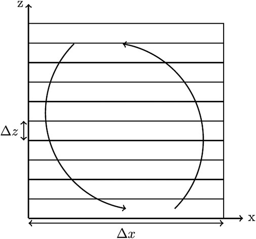
FIGURE 1. Schematic turbulent eddy simulated by a non-local mixing length over the grid of a large scale model.

Local formulations of the mixing lengths can be based on the local vertical wind shear (Hunt, 1988; Tjernström, 1993; Schumann and Gerz, 1995; Grisogono and Enger, 2004; Grisogono and Belušić, 2008; Grisogono, 2010; Venayagamoorthy and Stretch, 2010). Recently, Rodier et al. (2017) (hereafter RM17) have improved BL89 to make it physically more accurate for all stratification conditions. Indeed, BL89 is infinite for neutral cases. However, in case of strong wind shear, the ABL turbulence is disorganized and the size of the turbulent eddies is reduced compared with a free-convective case. In order to reproduce the shear-induced vertical disorganization of the free-buoyancy eddies, RM17 integrates the local vertical wind shear within the original BL89 formulation. The size of the largest ABL eddies in RM17 becomes:

$\{\begin{array}{l}e\left(z\right)=\underset{z}{\overset{z+l_{up}^{RM17}}{{\displaystyle \int }}}\beta \left({\theta }_v\left(z^{\prime }\right)-{\theta }_v\left(z\right)+C_0\sqrt{e}\sigma \left(z^{\prime }\right)\right)d{z}^{\prime }\\ e\left(z\right)=\underset{z-l_{down}^{RM17}}{\overset{z}{{\displaystyle \int }}}\beta \left({\theta }_v\left(z^{\prime }\right)-{\theta }_v\left(z\right)+C_0\sqrt{e}\sigma \left(z^{\prime }\right)\right)d{z}^{\prime }\end{array}$

where $C_0$ is a constant and $\sigma =\frac{\partial \left|\right|U\left|\right|}{\partial x_j}$ is the local vertical wind shear.

The mixing length is then:

$L_{RM17}={\left(\frac{l_{up}^{RM17-2/3}+l_{down}^{RM17-2/3}}{2}\right)}^{-3/2},(3)$

Redelsperger et al. (2001)correction is applied in the first 25 m of the model to improve the representation of the wind profile in the surface boundary layer. Moreover, Rodier et al. (2017) promoted the use of a dissipation constant ($C_{\mathit{ϵ}}$) reduced from 0.85 (in Bougeault and Lacarrère, 1989) to 0.34.

2.2 Large-Eddy Simulation Mixing Lengths

Large-Eddy simulations (Lilly, 1967; Deardorff, 1980; Pope, 2000) resolve most of the turbulence scales. LES are commonly used as a state-of-the-art numerical tool in order to study turbulence or to develop and evaluate parameterizations (Couvreux et al., 2010; Rio et al., 2010).

In LES, the grid is much smaller than the largest turbulent eddies and the nearly cubic grid fits the residual isotropic subgrid turbulence (see Figure 2). In this case, the most energy-containing subgrid eddies have the size of the grid box:

$L_{DELT}={\left(\text{Δ}x\text{Δ}y\text{Δ}z\right)}^{1/3},(4)$

where $\text{Δ}x$, $\text{Δ}y$ and $\text{Δ}z$ are the grid cell dimensions.

FIGURE 2

FIGURE 2. Schematic turbulent eddy simulated by a local mixing length in a LES grid.

This mixing length (hereafter $L_{DELT}$) is prescribed in most LES. However, close to the surface or in very stably stratified cases, the most energy-containing subgrid eddies may be smaller than the grid cell size. This is why Deardorff (1980) mixing length (hereafter DEAR) takes the stratification into consideration:

$L_{DEAR}=min\left({\left(\text{Δ}x\text{Δ}y\text{Δ}z\right)}^{1/3},0.76\sqrt{\frac{e}{N^2}}\right),(5)$

where N is the Brunt-Väïsälä frequency.

2.3 A New Mixing Length From Micro to Large Scales

None of the above-described mixing lengths are adapted to the gray zone of turbulence. Indeed, $L_{RM17}$ or $L_{BL89}$ hardly adapt to the horizontal resolution, a crucial element in the gray zone when subgrid turbulence mixing must be smaller than the one at large scale. Concerning $L_{DELT}$ and $L_{DEAR}$, they both depend on the vertical resolution which limits the turbulence mixing, as in Figure 3, whereas subgrid non-local structures exist in the gray zone of turbulence (Shin and Hong, 2014; Honnert et al., 2016).

FIGURE 3

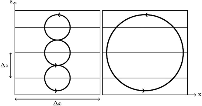
FIGURE 3. Schematic turbulent eddy in the gray zone of turbulence when the mixing length depends on $\text{Δ}z$(left) or not (right).

With $L_{DELT}$, the mixing length formulation takes into account the vertical resolution $\text{Δ}z$. In meteorological models, $\text{Δ}z$ is smaller than the horizontal resolution in Eq. (4) and limits $L_{DELT}$ (see Figure 3). We propose to use a non-local mixing length $\mathfrak{L}$ , which combines $L_{RM17}$ with a LES-adapted mixing length $L_{\text{Δ}}$ (Eq. 6) that avoids the purely numerical dependency of the mixing length to the model vertical discretization:

$L_{\text{Δ}}={\left(\text{Δ}x\text{Δ}y\right)}^{1/2},(6)$

$\mathfrak{L}$ is the minimum mixing length between the horizontal grid cell $L_{\text{Δ}}$ and $L_{RM17}$:

$\mathfrak{L}=min\left(\alpha L_{\text{Δ}},L_{RM17}\right),(7)$

where α is a tuning parameter set to 0.5, according to the numerical experiments detailed in Section 4.3. This formulation is continuous and does not overshoot. Usually, $L_{RM17}$ is of the order of the boundary layer height (but smaller). $\mathfrak{L}$ is equal to $L_{RM17}$ for large horizontal grid meshes. At the surface, $L_{RM17}$ is smaller than $L_{\text{Δ}}$ as it is limited by the distance to the surface. For LES (cubic) grid meshes, $\mathfrak{L}$ is equivalent to Deardorff: the base mixing length is the horizontal grid mesh and it is limited by a stability-based length (RM17), as done in Deardorff length by the TKE part (see Eq. 5) but taking into account shear as well. For grid meshes in the gray zone of turbulence, this is the smaller of the two.

The $\mathfrak{L}$ mixing length only depends on the horizontal grid mesh (which is a key element to define where we stand in regards to the gray zone) and the atmospheric conditions (buoyancy and shear). $\mathfrak{L}$ is independent of the vertical grid chosen.

3 Model, Case Studies and Evaluation Method Description

3.1 Model

The model used in the present work is the atmospheric non hydrostatic research model Meso-NH (Lac et al., 2018). It is used here from LES to hectometric scales in idealized frameworks. The spatial discretization is based on the C grid of Arakawa with Cartesian coordinates. The advection scheme for momentum variables is a centered scheme of 4th order in space, and a Runge–Kutta time-splitting of 4th order in time, well adapted to LES as the effective resolution is $5-6\text{Δ}x$ (Lac et al., 2018). For potential temperature and hydrometeor mixing ratios, the advection scheme is PPM (Piecewise Parabolic Method) from Colella and Woodward (1984). A numerical diffusion is added to filter the shortest wavelengths and avoid energy accumulation in the tail of the energy spectrum. It is set using a characteristic time (e-folding time) applied to the momentum variables. The atmospheric model is coupled with the EXternalized SURFace (SURFEX) model (Masson et al., 2013). The turbulence scheme is based on CBR (Cuxart et al., 2000), which is a 1.5 order turbulence parameterization based on a TKE prognostic equation, where the eddy-diffusivity, $K_{\varphi }$, depends on the TKE and a mixing length l:

$K_{\varphi }=c_{\varphi }\times l\times \sqrt{e},(8)$

where $c_{\varphi }$ is a constant depending of ϕ and e is the TKE.

At mesoscale resolutions (horizontal mesh larger than 1 km), it can be assumed that the horizontal gradients and the horizontal turbulent fluxes are much smaller than their vertical counterparts: they are therefore neglected (except for the advection of TKE) and the turbulence scheme is used in its 1D version, as in AROME (Seity et al., 2011). At finer resolution, the whole subgrid equation system is considered in its 3D version, as it is the case in the present work. The microphysical scheme is a mixed-phase one moment scheme (Pinty and Jabouille, 1998) which considers three solid (ice crystal, snow, and graupel) and two liquid (cloud droplets and raindrops) hydrometeors. The radiation parameterizations come from ECMWF, and include the Rapid Radiation Transfer Model (Mlawer et al., 1997) for long-wave and Fouquart and Bonnel (1980) for shortwave radiations.

3.2 Case Studies and LES Specifications

Boundary-layer turbulence comes from boundary-layer convection (thermal-induced turbulence) and wind shear (dynamical-induced turbulence). Three cases combining differently one or the other source of turbulence are evaluated here, in dry or cloudy conditions. For all cases, the reference LES is run with $L_{DEAR}$ at high resolution.

3.2.1 Free Convective Boundary Layer

The first case is a free convective boundary layer (CBL). It is based on radio-soundings collected during the International ${\mathrm{H}}_2$O project (${\text{IHOP}}_{2002}$) campaign (Weckwerth et al., 2004). In this work, we reproduce the June 14th, 2002 case, corresponding to a growing CBL near Homestead, Oklahoma (Couvreux et al., 2005). This day is characterized by high pressure (1,016 hPa or more) and light wind (＜5 m s⁻¹). The weak vertical shear guarantees a free convective case. The well-mixed boundary layer reaches 1.2 km in the beginning of the afternoon. This case is chosen as it presents a relatively uniform site topography and a development of a typical continental CBL. The numerical domain is a 16 × 16 km² area. Lateral boundary conditions are periodic. Seven hours of dynamics are reproduced. The horizontal grid mesh for the LES is 50 m. The vertical grid is stretched, but the spacing is always ＜100 m in the ABL, so that the grid boxes are close to cubes. The numerical diffusion is small, the time at which the $2\text{Δ}x$ waves are damped by the factor $e^{-1}$ is equal to 1800s. The diffusion value is identical for all resolutions and tested mixing lengths, allowing to compare the results.

3.2.2 Neutral Boundary Layer

The second case is a neutral boundary layer corresponding to the incoming flow conditions of case 2681829 of the Mock Urbain Setting Test experiment (hereafter must, Yee and Biltoft, 2004). This near full-scale experiment was conducted during September 2001 in Utah’s West desert, at US Army Dugway Proving Ground. The site is located 1310 m above the mean sea level and can be considered as flat and homogeneous. MUST, starting the September 25, 2001 at 1830 LT (local time = UTC$-$6 h), is characterized by a neutral state atmosphere, a strong wind ($\approx$8 m s⁻¹ at z = 4 m height) and a shear-induced turbulence. This case is chosen as it represents a typical continental neutral boundary layer. Moreover, this case is of particular interest for further developments of the Immersed Boundary Method (IBM) version of the Meso-NH (MNH-IBM, Auguste et al., 2019). The numerical domain is a 40 km side square. The vertical elevation of the domain goes up to 1500 m high. The first vertical layer measures 10 m high. The vertical grid size increases linearly with a geometric ratio of 1.09 and reaches it maximum value ($\text{Δ}z=50$ m) at the elevation of 500 m. The vertical grid spacing remains constant between 500 m and the top of the domain. The ground friction is characterized by a roughness length $z_0$ = 0.045 m and modeled with SURFEX. An imposed geostrophic wind maintains the flow. Near the ground, the wind conditions match the observations: the wind speed is around 9 m s⁻¹ at z = 10 m and the wind direction has an angle of −41° with respect to the x-axis. The case is purely neutral. The $\mathrm{ℒ}$ mixing length is tested at 50, 100, 200 and 400 m horizontal resolutions and compared with the reference LES at 50 m. The sensitivity of the results to α is also investigated. The tuning of the numerical diffusion is the same as for the IHOP case.

3.2.3 Cold Air Outbreak

The third case is a cold air outbreak. Cold-air outbreaks are large-scale cold air masses over relatively warm waters. This phenomenon is common in the North Atlantic during winter (Field et al., 2014). The CONSTRAIN campaign (Field et al., 2014) studied cold air outbreaks in the North Sea involving a complex microphysics with mixed phases of ice and liquid water and mesoscale 2D (cloud streets) or 3D (open cells) structures. Several models inter-comparisons have been conducted on this study-case: an inter-comparison of global (Tomassini et al., 2016), limited area models (Field et al., 2017) and LES simulations (de Roode et al., 2019). The present case is described in de Roode et al. (2019). It corresponds to a transition from stratocumulus to cumulus as the cloud deck is advected over an increasingly warmer sea surface temperature. This simulation combines turbulence from thermal and dynamical origins, as well as presence of clouds. Similarly to de Roode et al. (2019), the top of the LES domain is at 5 km, with a vertical grid spacing of 25 m between the surface and 3 km and stretched above. The simulations covers an area of 96 × 96 km² and last 14 h (from 00 to 14UTC). In the present paper, the LES is run at 62.5 m (instead of 250 m in de Roode et al. (2019)) to insure LES conditions. In de Roode et al. (2019), due to the Louis (1979) parameterization, Meso-NH produced too strong heat surface fluxes compared with other simulations of the inter-comparison. Here, this point is improved by using the iterative method proposed by Fairall et al. (2003) to produce sea surface fluxes. Moreover, the present microphysics considers the mixed phase while most of de Roode et al. (2019) simulations were based on the warm case. In this paper, several mixing lengths ($\mathfrak{L}$, $L_{BL89}$, $L_{RM17}$ and $L_{DEAR}$) are tested at 125, 250 and 500 m grid spacing and compared with the reference LES. We focus on two moments: t = 2 h, when stratocumulus evolve toward open cells, and t = 12 h, when cumulus clouds are well developed. Compared with the previous cases, the numerical diffusion is slightly more active, with the time at which the $2\text{Δ}x$ waves are damped by the factor $e^{-1}$ equal to $500s$.

3.3 Simulations at Gray Zone Resolutions and Their Evaluation

According to Honnert et al. (2011), the gray zone of turbulence ranges between 0.2 and 2 times the boundary-layer height for CBL. The boundary-layer height being about 1.5 km for both IHOP and CONSTRAIN experiments, horizontal resolutions between 100 and 500 m are therefore considered as in the gray zone of turbulence. For neutral cases, Honnert (2018) has shown that the gray zone of turbulence ranges between 0.03 and 1 times the boundary-layer height. For MUST, the boundary layer is of 1500 m in height and horizontal resolutions between 50 and 400 m are considered as in the gray zone of turbulence.

In kilometric-scale simulations, non-local schemes such as mass-flux schemes (Hourdin et al., 2002; Siebesma et al., 2004; Pergaud et al., 2009) are used to represent the non-local turbulence of CBLs. However, Honnert et al. (2011) proved that mesoscale mass-flux schemes are too diffusive in the gray zone of turbulence and cannot be used at hectometric scales. In addition, the presence of a non-local turbulence scheme would distort the new mixing length impact analysis on the turbulence scheme. This is the case even if the influence of the non-local scheme would be very reduced as in non-local schemes dedicated to the gray zone (Boutle et al., 2014; Honnert, 2016). In the present paper, all simulations are therefore undertaken without any additional non-local boundary-layer scheme. We will focus on resolutions between LES and 500 m (upper gray-zone). The $\mathfrak{L}$ mixing length is assumed to naturally work at mesoscale and large scale because it is then equal to the uni-dimensional mixing length $L_{RM17}$.

This study does not use direct observations. However, as seen in the previous section, the test cases come from intercomparison studies, meaning that they are close but simplified compared with the reality. We have respected the intercomparison setup where the LES simulations have been validated compared with the observations, allowing the use of those LES as a reference for the evaluation of the new mixing length simulations.

Quantification of the resolved and subgrid fluxes are key points for the parameterization evaluation in the gray zone. Honnert et al. (2011) use the coarse-graining of LES fields in order to quantify the ‘true’ resolved and subgrid part of the turbulence in the gray zone. It appears that the partitioning between subgrid and resolved fluxes in the mixed layer of CBLs follows one unique function depending only on $\frac{\sqrt{\text{Δ}x\text{Δ}y}}{h}$. This function is quantified in Honnert et al. (2011) and called partial similarity function. In this work, simulations with $\mathfrak{L}$, $L_{DEAR}$ and $L_{RM17}$ in the gray zone are compared with LES results and partial similarity functions.

4 Results

4.1 Free Convective Boundary Layer

4.1.1 Boundary-Layer Height

Figure 4 shows the boundary-layer height computed from the IHOP simulations at resolutions ranging from 50 to 500 m. Three different mixing lengths are used: $\mathfrak{L}$, $L_{DEAR}$ and $L_{RM17}$. The boundary-layer height is computed as the maximum of the potential temperature gradient during the 7 h simulated.

FIGURE 4

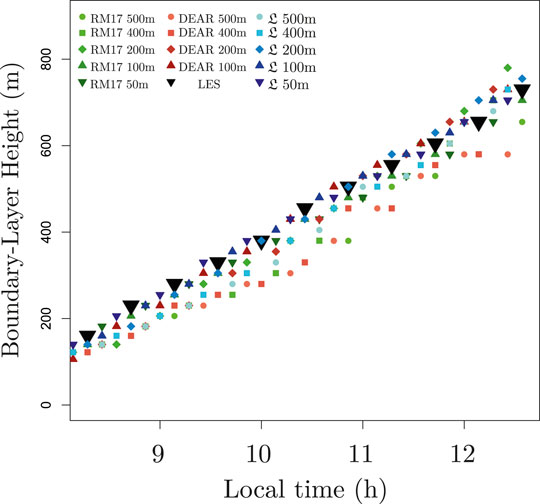
FIGURE 4. Time evolution of the boundary-layer height for the IHOP case run with RM17, DEAR and $\mathfrak{L}$ at 50, 100, 200, 400, and 500 m grid spacing.

During the first 5 h of dynamics and for all the configurations, the boundary layer height growth rate is similar to the reference LES (dark triangles in Figure 4) but with slightly lower values. Then, the growth of the CBL slows in the LES, which is not the case in high resolution simulations using $L_{RM17}$ and $L_{DEAR}$. Table 1 presents the bias and standard deviation of the simulations compared with the LES. Simulations using $\mathfrak{L}$ have the smallest bias at resolutions smaller than 200 m whereas simulations using $L_{RM17}$ have the smallest bias at resolutions coarser than 200 m. If the boundary layer develops correctly whatever the configuration, simulations using $\mathfrak{L}$ are in better agreement with the LES than those using $L_{DEAR}$. In particular, $L_{DEAR}$ produces a too low boundary-layer height at hectometric scales in agreement with Honnert et al. (2011).

TABLE 1

TABLE 1. Bias and standard deviation (separated by a $/$) of the boundary-layer height (in meters) for the IHOP case.

4.1.2 Partial Similarity Functions

At the mesoscale, the turbulence is entirely subgrid and the boundary-layer eddies are smaller than the resolution of the model. In LES, the turbulence is mainly resolved, as it explicitly represents the largest and most energetic turbulent eddies. In-between, in the gray-zone of turbulence, the subgrid/resolved partitioning of the TKE follows the partial similarity function from Honnert et al. (2011). Figure 5 presents this subgrid/resolved TKE partitioning for the different IHOP simulations undertaken as a function of $\text{Δ}x/h$. In the mixed layer of a clear-sky convection boundary-layer, the subgrid/resolved partitioning only depends on the model resolution (whose proxy is the model horizontal grid spacing) and on the size of the largest boundary-layer eddies (whose proxy is the boundary-layer height, assuming that, the higher the boundary-layer eddies, the coarsest they are). More details can be found in Honnert et al. (2011) or Shin and Hong (2014).

FIGURE 5

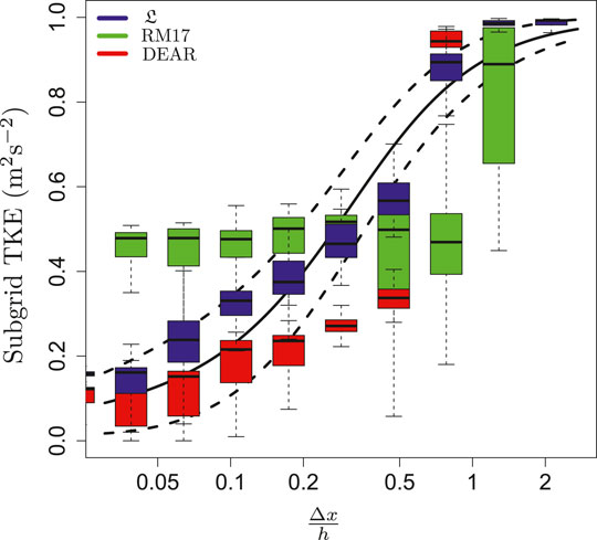
FIGURE 5. Subgrid TKE as a function of the resolution normalized by the ABL height for IHOP simulations undertaken with RM17 (in blue), DEAR (in green) or $\mathfrak{L}$ (in red). The reference partial similarity function for the TKE and the uncertainty margins are represented by the full and dashed black lines, respectively.

The black line in Fig. 5 is the partial similarity function of the TKE. The dashed lines are the first and the last vigintiles of the coarse-grained LES data. They represent the allowed margin of error. The data obtained with simulations using $L_{RM17}$, $L_{DEAR}$ and $\mathfrak{L}$ as mixing length are shown in blue, green and red, respectively. $L_{RM17}$ produces a correct subgrid/resolved partitioning for boundary-layer height smaller than the grid spacing $\left(\frac{\text{Δ}x}{h}>1\right)$. Otherwise $\left(\frac{\text{Δ}x}{h}<1\right)$, the subgrid part of the TKE drops at about 0.6 times the total TKE. This is particularly unrealistic in LES where the TKE should be resolved when $\frac{\text{Δ}x}{h}<0.05$. $L_{RM17}$ presents also inconsistency in the gray zone: the TKE is either too subgrid for $\frac{\text{Δ}x}{h}<0.2$, or too resolved for $\frac{\text{Δ}x}{h}>0.3$. On the contrary, simulations with $L_{DEAR}$ correctly follow the partial similarity function when $\frac{\text{Δ}x}{h}<0.1$ but are always too resolved in the gray zone. Finally, simulations using $\mathfrak{L}$ follow the partial similarity function until $\frac{\text{Δ}x}{h}\approx 0.4$ but are too resolved for $0.4<\frac{\text{Δ}x}{h}<0.5$. This may be due to the fact that a non-local part of the turbulence is still necessary for resolutions between 400 and 500 m (see Honnert et al., 2016).

It has been found (not shown in Figure 5) that the subgrid TKE evolution as a function of $\frac{\text{Δ}x}{h}$ presents very few differences between BL89 and RM17. The impact of the wind shear on turbulence is generally quantified by the $-h/L_{MO}$ ratio, where $L_{MO}$ is the Monin–Obukhov length. For moderate and strong winds, if $-h/L_{MO}>10$ the dynamical production is negligible. In IHOP, $-h/L_{MO}$ is close to 100 (see Honnert et al., 2011) for more details) explaining why BL89 and RM17 show similar results.

4.1.3 Spectral Analysis

In order to complete this analysis, Figure 6 presents the energy spectra after 6 h of dynamics, using $\mathfrak{L}$ or $L_{DEAR}$. The spectra are computed from data over all the levels between the surface and the top of the boundary layer. Simulations using $L_{RM17}$ are not shown because whatever the resolution, the TKE is not resolved enough to perform a spectral analysis.

FIGURE 6

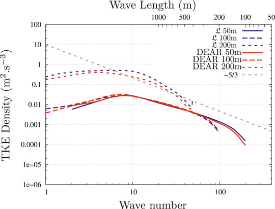
FIGURE 6. IHOP horizontal TKE spectral analysis, inside the boundary layer and at 13 local hour of dynamics, for simulations undertaken with $L_{DEAR}$ (in red) and $\mathfrak{L}$ (in blue) at 50, 100, and 200 m grid spacing. The gray dashed line is the Kolmogorov $-5/3$ slope.

In Fig. 6, the gray dashed line is the Kolmogorov $-5/3$ slope. The full and dashed lines represent the energy spectra undertaken with $L_{DEAR}$ and $\mathfrak{L}$, respectively. There is no significant difference between DEAR and the new mixing length at the finest resolutions. At 50 m grid spacing, $\mathfrak{L}$ produces energy spectra in agreement with DEAR, considered as the LES reference. The most significant difference is found at 200 m grid spacing where it is clear that DEAR produces too much resolved turbulence compared with the LES and the Kolmogorov theoretical references. $\mathfrak{L}$ improves the representation of the turbulence at this resolution.

4.2 Neutral Boundary Layer: Resolved TKE Vs. Coarse-Grained LES

The neutral MUST case allows to examine the behavior of the mixing lengths in the fine resolution part of the gray zone of turbulence. Figure 7 shows the vertical profiles of total (left column) and resolved (right column) TKE obtained for the MUST case. The reference LES (50 m grid spacing with DEAR) is represented by the solid black lines. Simulations are undertaken at four horizontal grid spacing (50, 100, 200, and 400 m) with three mixing lengths, $L_{DEAR}$ (red lines), RM17 (green lines) and $\mathfrak{L}$ (blue lines).

FIGURE 7

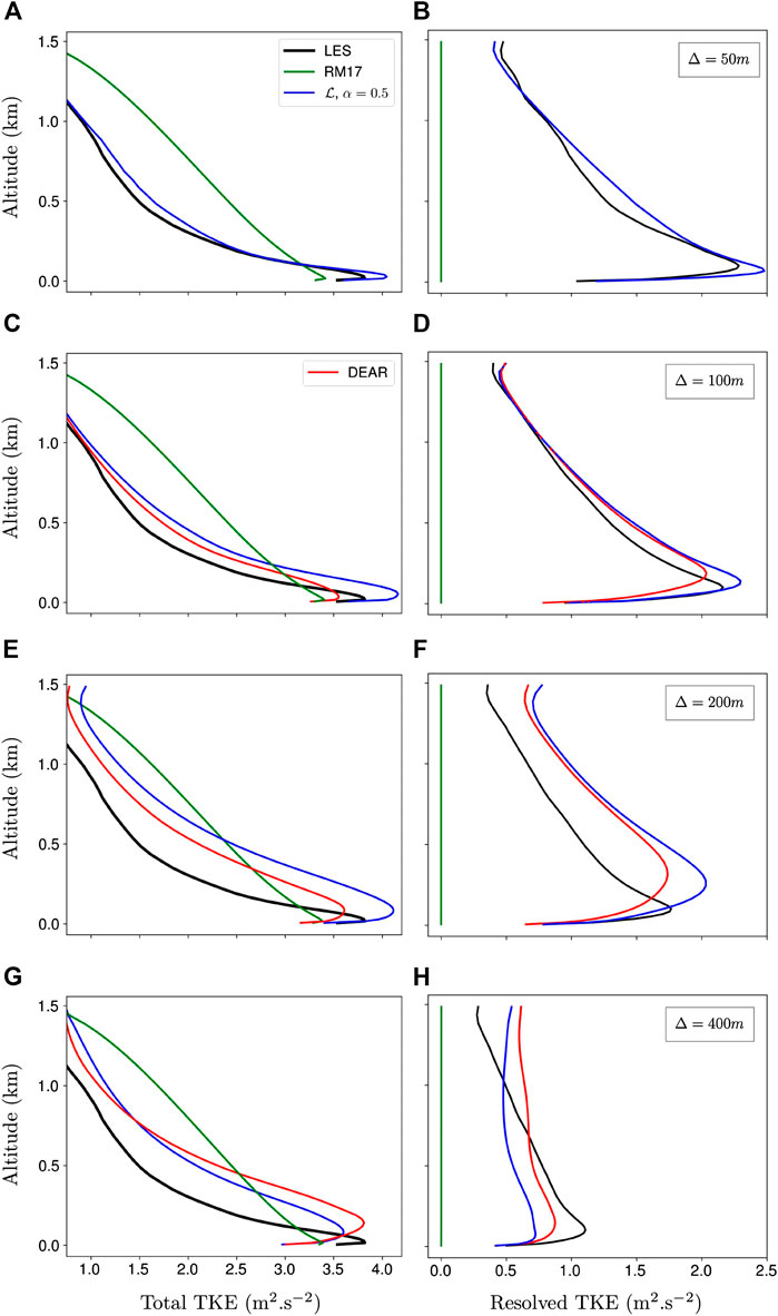
FIGURE 7. Vertical profiles of total (left column) and resolved (right column) TKE obtained in the MUST neutral configuration from LES (black), RM17 (yellow), $L_{DEAR}$ (red) and $\mathfrak{L}$ (blue) at 50, 100, 200, and 400 m horizontal resolution.

Focusing on the coarse-grained LES results, the TKE is more resolved at the finer resolutions. For instance, TKE is twice more resolved at 100 than at 400 m grid spacing. For all resolutions, no resolved TKE is obtained with RM17. In this neutral case, where sources of instabilities are smaller than in convective cases, the subgrid mixing of RM17 inhibits the resolved movements, even at finest resolutions. This highlights the need of using an appropriate mixing length in the gray zone.

At 50 m grid spacing, the good agreement between LES and $\mathfrak{L}$ energy profiles for the resolved (Figure 7b) and total TKE (Figure 7a) shows that the new mixing length can be used at high resolution and does not present inconsistency compared with the reference LES. For resolved TKE at coarser resolutions (100 m, Figure 7d, 200 m Figure 7f), $\mathfrak{L}$ is almost similar, but more resolved than DEAR. The agreement compared with the coarse-grained LES is satisfactory especially at 100 m grid spacing. At 400 m grid spacing (Figure 7h), both $\mathfrak{L}$ and DEAR overestimate the resolved TKE above 1,000 and 750 m, respectively and underestimate it below. This underestimation is more pronounced with $\mathfrak{L}$, especially close to the ground and DEAR is in better agreement with the coarse-grained LES. Nonetheless, $\mathfrak{L}$ agreement with the coarse-grained LES remains satisfactory in the fine resolution part of the gray zone of turbulence.

The results are similar for the total TKE (Figs 7c, 7e, 7g). $\mathfrak{L}$ and DEAR are close one to the other and in much better agreement with the LES results than RM17.

4.3 Sensitivity Tests to α

The new mixing length $\mathfrak{L}$ aims to model the turbulent mixing whatever the resolution or the meteorological conditions within the boundary layer. Therefore, the tuning coefficient α should not vary. However, it has to be set. This setting could depend on the atmospheric model in which it is used and more particularly of its intrinsic diffusion properties. In the present work, we will find a compromise to set the value of α for CBR turbulence scheme using the Meso-NH model.

The effective resolution of a model (Skamarock, 2003; Ricard et al., 2013) is the minimum wavelength correctly seen by the model. Due to the physical and numerical diffusion, it is always larger than the grid size ($\text{Δ}x$). This effective resolution depends on several parameters: the model considered (more particularly the chosen dynamical scheme), the physical schemes, the internal adjustments of these different schemes and finally the meteorological situation itself. For example, the turbulent diffusion is governed by the chosen mixing length, but also by the other scheme coefficients, such as the turbulence dissipation coefficient. The more diffusive a model, the greater the effective resolution compared to $\text{Δ}x$. Meso-NH with the numerical schemes used in this study presents an effective resolution of 5 $\text{Δ}x$ (Lac et al., 2018) which is the signature of a good accuracy of the numerical schemes. Figure 6 confirms an effective resolution less than 5 $\text{Δ}x$, i.e. the scale from which the model departs from the theoretical slope of $-5/3$. The effective resolution of the model is a main characteristic of the resolved/subgrid partition of the simulations. The theoretical subgrid/resolved partition of Honnert et al. (2011) is obtained from a coarse-graining which gives results from the LES perfect fields. To adjust the parametrization of the mixing length to the diffusion characteristics of the model, a tuning parameter is needed, that is α in Eq. 7.

In IHOP and MUST, the value of α was set to 0.5. The sensitivity of these cases results to α is here investigated. Figure 8 shows the subgrid TKE as a function of $\frac{\text{Δ}x}{h}$ for IHOP (left) and MUST (right) simulations undertaken with α ranging from 0.33 to 1. The black line is the TKE reference partial similarity function from Honnert et al. (2011). The uncertainty margins are represented by the black dashed lines.

FIGURE 8

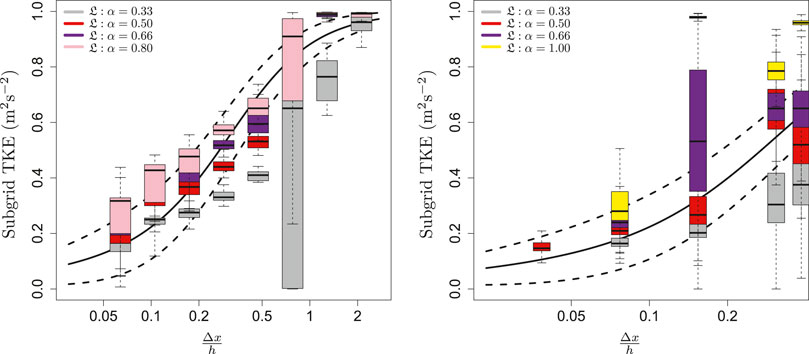
FIGURE 8. Sensitivity test to the α from 0.33 to 1 in IHOP (left) and MUST (right). The subgrid TKE is represented as a function of the resolution normalized by the ABL height. The reference partial similarity function for the TKE (Honnert et al., 2011) and the uncertainty margins are represented by the full and dashed black lines, respectively.

Concerning IHOP, Figure 8 left shows that, for the small values of $\frac{\text{Δ}x}{h}$ (i.e., LES regime), large values of α result in diffusive simulations. The subgrid turbulence is too large and the simulation never enters the LES regime because the turbulence is not resolved enough. At the meso-scale (i.e., for large values of $\frac{\text{Δ}x}{h}$) the turbulence is entirely subgrid for all values of α. The mixing length is used in the computation of the fluxes, but also in the parameterization of the diffusion. This is particularly obvious in the gray zone, where the larger α, the more diffusive the result is. Moreover, for $\alpha =0.33$ there is not enough diffusion so that resolved turbulence structures appear even at a 2 km grid spacing ($\frac{\text{Δ}x}{h} \approx 1.3$), which is in contradiction with the reference partial similarity function. Extreme values of α ($\alpha =0.33$ and $\alpha =1$) show also a large variability around $\frac{\text{Δ}x}{h}=0.8$ which is due to waves development in the simulations.

For the MUST case (see Figure 8 right), similarly to IHOP in LES regimes and in the gray-zone, large values of α ($\alpha =0.66;1$) result in more diffusive simulations. If subgrid turbulence is small enough to maintain simulations in the LES regimes for $\frac{\text{Δ}x}{h}<0.1$, this is not the case for larger $\frac{\text{Δ}x}{h}$ values and results are outside the uncertainty margins.

Globally, extreme values of α should be avoided. For MUST, the best agreement with the reference partial similarity function is obtained with $\alpha =0.5$, whereas $\alpha =0.66$ seems to be better for IHOP. However the value of $\alpha =0.5$ is a good compromise for the two cases, and makes it possible to have a resolved TKE closer to the theoretical curb in LES regime. Therefore, $\alpha =0.5$ is retained as the default value in Eq. 7.

4.4 Cloudy Evolving Boundary Layer

In the previous section, α has been tuned on idealized cases of convective (IHOP, in Section 4.1) and neutral (MUST, in Section 4.2) boundary layers. In this section, $\mathfrak{L}$ is tested on a cloudy evolving boundary layer.

4.4.1 Ability to Reproduce the Cloud Types and Large Scales

The CONSTRAIN case is more critical as it combines turbulence from thermal and dynamical origins, as well as presence of mixed clouds. CONSTRAIN was held in the North of Scotland. The simulation begins at 00 UTC - 1 local hour.

Figure 9 shows the cloud top and base temporal evolution in simulations undertaken with DEAR, RM17 and $\mathfrak{L}$ at 125, 250, and 500 m grid spacing. Results are compared with the LES reference (in black) at 62.5 m grid spacing. The cloud base is well represented whatever the resolution and the mixing length. For all resolutions and simulation times, the boundary-layer height is well recovered although BL89 and RM17 result in a too shallow boundary layer at 125 m grid spacing (see also Figure 10).

FIGURE 9

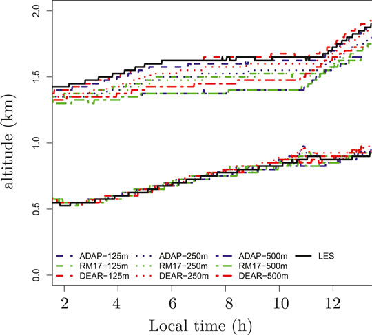
FIGURE 9. Temporal evolution of the cloud base and cloud top in CONSTRAIN with DEAR, RM17 and $\mathfrak{L}$ (red, green and blue lines, respectively) at 125, 250, and 500 m grid spacing (full, dashed and dotted lines, respectively).

FIGURE 10

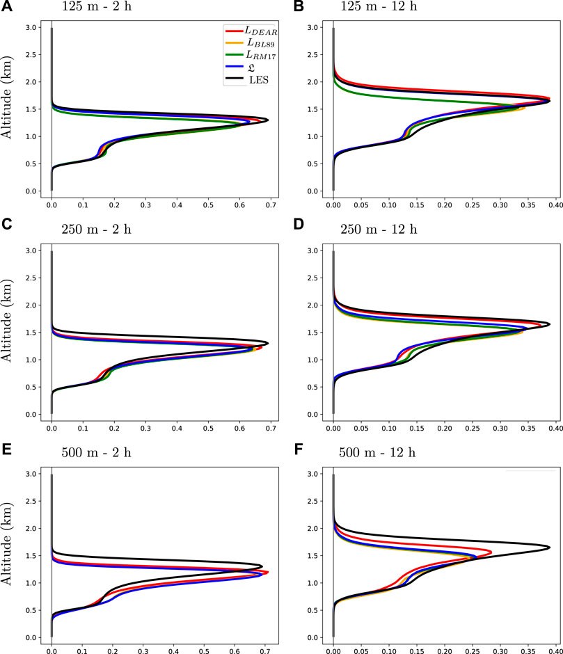
FIGURE 10. Vertical profiles of mean cloud fraction for CONSTRAIN simulations at 2 h (left column) and 12 h (right column) at the grid spacing of 125 m (top row), 250 m (middle), 500 m (bottom row) with DEAR (in red), BL89 (in orange), RM17 (in green), $\mathfrak{L}$ mixing length (in blue) and the reference LES coarse-graining (black).

Figure 10 shows the vertical profiles of mean cloud fraction produced by the different mixing lengths in the stratocumulus stage (2 h local hour) and the cumulus stage (12 h local hour). One can see a good transition from stratocumulus to cumulus at 12 h for all simulations, with a decreasing cloud fraction and an increasing cloud depth (see Figure 9). Moreover, the different simulations produce a correct maximal cloud fraction in the stratocumulus stage despite a too low maximal cloud fraction at large scales (cf. Figure 11a). The maximal cloud fraction is also well-reproduced by $\mathfrak{L}$ at fine resolution in the cumulus stage (Figure 11b). However, for all the mixing length, almost half of the cloud fraction is missing at 500 m grid spacing at 12 h (Figure 11f).

FIGURE 11

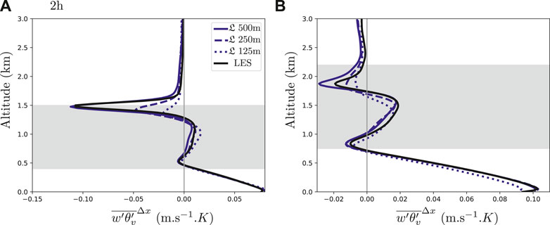
FIGURE 11. Vertical profiles of total $\overline{w^{\prime }{\theta }_v^{\prime }}$ from LES (solid line) and $\mathfrak{L}$ (dashed lines) at 125, 250, 500 m grid spacing at 2 h (A) and 12 h (B).The gray area represents the cloud layer in the LES.

The main problem is that the coarser the resolution, the lower the cloud top (Figure 9). This can be mainly explained by the fact that the simulations do not have any non-local turbulence scheme such as a mass-flux scheme, limiting the cloud development.

During the first hours of the LES simulation $L_{MO}$ is close to 300 m, the boundary-layer height is about 1.2 km and rolls appear in the simulations. The buoyancy flux is a quantity of particular interest in order to verify the schemes ability to reproduce the convective rolls of stratocumulus (at t = 2 h, see Figure 10a) and cells of cumulus (at t = 12 h, see Figure 10b). As explained in de Roode et al. (2019), the two minima of $\overline{w^{\prime }{\theta }_v^{\prime }}$ show negative values that will act as a sink term of TKE and impact the future development of both the stratocumulus and the cumulus layers. In the stratocumulus case, the cloud-base minimum is small and well-represented by $\mathfrak{L}$ at all resolutions. The minimum of $\overline{w^{\prime }{\theta }_v^{\prime }}$ at the cloud top is gradually less negative as resolution decreases. In the cumulus case, the boundary-layer, the cloud layer and the cloud top are well-represented by $\mathfrak{L}$ at all resolutions, especially the minimum at the cloud base showing the decoupling between the cloud and the surface. The largest variability of $\overline{w^{\prime }{\theta }_v^{\prime }}$ between the resolutions is obtained at the cloud top associated to the entrainment, but $\mathfrak{L}$ at 500 m succeeds to reproduce this process.

4.4.2 Resolved TKE Vs. Coarse‐Grained LES

Figure 12 shows the resolved TKE produced by the different mixing lengths in the stratocumulus stage and the cumulus stage of CONSTRAIN. Focusing on the results of the coarse-graining LES (in black), it is observed that, similarly to the neutral case, the finer the resolution, the larger the resolved TKE. Contrary to the buoyancy where only a small sensitivity to the resolution has been observed, TKE is half less resolved at 500 m than at 125 m grid spacing.

FIGURE 12

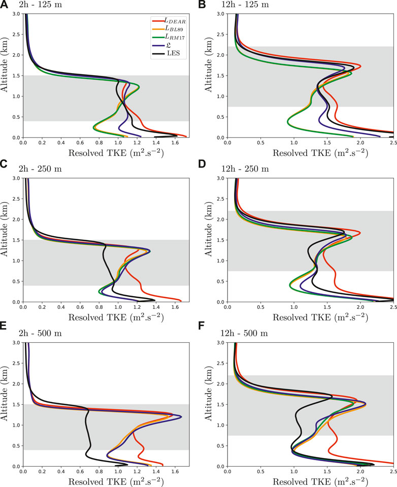
FIGURE 12. Vertical profiles of TKE for CONSTRAIN simulations at 2 h (left column) and 12 h (right column) at the resolutions of 125 m (top row), 250 m (middle), 500 m (bottom row) with DEAR (in red), BL89 (in orange), RM17 (in green), $\mathfrak{L}$ mixing length (in blue) and the reference LES coarse-graining (black).The gray area represents the cloud layer.

By construction, the $\mathfrak{L}$ mixing length (in blue) depends on RM17 and DELT (close to DEAR). Figure 12 shows that the vertical profiles obtained with $\mathfrak{L}$ are well located between those obtained with DEAR (in red) and RM17 (in green). More precisely, at high resolution (125 m grid spacing, Figures 12a,b) $\mathfrak{L}$ mimics the behavior of DEAR when it mimics the behavior of BL89 and RM17 at 500 vm (Figures 12e,f).

In the stratocumulus stage (see Figures 12a,c,e), the $\mathfrak{L}$ mixing length reproduces well the LES reference (in black) in the lower part of boundary layer. It is more difficult for this new mixing length to represent the stratocumulus cloud layer at 250 and 500 m, probably because neither $L_{DEAR}$ nor $L_{RM17}$ are able to reproduce the characteristics of the stratocumulus at these resolutions. It should be noted that even in the cloudy part, $\mathfrak{L}$ provides the profile closest to the reference. Be aware that we do not comment on the very first levels of the model, where the turbulence is mainly subgrid even with LES grid cells: as the turbulence is not mainly resolved, the LES cannot be considered as a good reference.

In the cumulus part (see Figures 12b,d,f), $\mathfrak{L}$ reproduces well the resolved TKE profiles both in the cumulus layer and in the underlying boundary layer, particularly at fine scales. However, the cumulus present too large resolved turbulence at 500 m leading to an underestimated subgrid entrainment (Figure 10b). We assume that there is a lack of non-local turbulence for this resolution, whereas the boundary-layer thermals that produce the non-local turbulence are fully resolved at finer scales (Shin and Hong, 2014). This problem cannot be fixed by the mixing length itself (cf. Section 5).

5 Discussion

As seen in this paper, $\mathfrak{L}$ can be used in the LES regime. This is because, in practice, $\mathfrak{L}$ and DEAR have the same behavior for all types of stability conditions. In unstable or neutral cases, DEAR is related to the grid size, which is equivalent to the use of the horizontal size of (LES nearly isotropic) grid meshes in $\mathfrak{L}$. In stable cases and in the inversion layers, DEAR limits the size of the eddies through a term accounting for the stratification. In $\mathfrak{L}$, the RM17 component plays this role (cf. Section 2.3).

Over complex terrain, Cuxart (2015) underlines that hectometric scales using a 3D turbulence scheme are not in the LES regime, since the resolved motions fall outside the inertial sub-range and follow the definition of Smolarkiewicz and Prusa (2002) of the “Very-Large Eddy simulation” (VLES). In the same vein, Efstathiou et al. (2018) identified a regime called near gray zone, where most of the TKE is resolved but for which these coarse LES simulations should not be considered as LES converging because their grid length is not fine enough to present a clear inertial sub-range (see Sullivan and Patton, 2011). In a way, this paper deals with these VLES or near-gray zone regimes and $\mathfrak{L}$ could be tested in cases of turbulence triggering at sun rise or turbulence in complex terrain.

The turbulence is not isotropic (as in LES) in the gray zone of turbulence, due to the residual traces of non-local turbulence. This is why Kitamura (2015) proposed two mixing lengths in the gray zone, one horizontal and one vertical. In the present paper, as in LES, the turbulence scheme is 3D isotropic at all resolutions by construction. $\mathfrak{L}$ is built to be used in isotropic schemes, in order to be compatible with LES current schemes. In our case, the anisotropy of the turbulent fluxes is entirely driven by horizontal or vertical gradients of the atmospheric quantities.

At kilometric-scales, $\mathfrak{L}$ behaves as $L_{RM17}$: it reproduces well the neutral boundary layer. However, in CBL simulations at resolutions coarser than 500 m, a non-local scheme remains necessary because $\mathfrak{L}$ alone is not able to reproduce the CBL like the combination of turbulence and mass-flux schemes would. We believe that with the adequate non-local scheme, $\mathfrak{L}$ can be used at all scales.

The value of the α tuning parameter has to be valid whatever the boundary layer stability as RM17 is supposed to adapt to the BL stability. However, when $\mathfrak{L}$ is used in an other model than Meso-NH, α may be different than 0.5. Although, $\mathfrak{L}$ is not very sensitive to the value of α around 0.5, the determination of the α value should be undertaken as any other tuning parameter of the given model.

6 Conclusion

This work seeks to improve the turbulence scheme at the gray zone of turbulence scales, particularly when the resolution is too coarse and the meshes too anisotropic for the LES configuration to give a good subgrid/resolved partitioning of the TKE. This article describes a new mixing length, $\mathfrak{L}$, built on a previously proposed approach to blend a LES and a mesoscale mixing length in order to produce the right amount of subgrid turbulence at hectometric scales:

$\mathfrak{L}=min\left(\alpha L_{\text{Δ}},L_{RM17}\right),(9)$

where α is a tuning parameter that may depend on the boundary layer characteristics (not on the resolution). The sensitivity test to α performed herein establishes $\alpha =0.5$ as the default value. In this formulation, the mixing length is smaller than the smallest of the two components. The merged mixing length does not explicitly depend on the model resolution, but in practice it increases with increasing grid size up to the mesoscale, giving it a self-adaptation faculty. $\mathfrak{L}$ is tested on three different boundary-layer cases and compared with LES and LES coarse-graining results. The first case, IHOP, represents a free-convective boundary layer, with no significant impact from the wind. In this case, the gray zone of turbulence and global parameters such as the boundary-layer height or the resolved/subgrid partition are well represented by the new mixing length. Secondly, MUST, a neutral case of purely dynamic turbulence is studied. In this case, the correct representation of subgrid/resolved partition at all scales allows a good representation of the wind profile. Finally, in CONSTRAIN, a case of stratocumulus to cumulus transition in a cold-air outbreak, the turbulence is well represented inside the boundary layer by $\mathfrak{L}$ in the gray zone of turbulence. This new isotropic turbulent mixing length can then be used for simulations of neutral and convective boundary layers ranging from the LES to meso-scale resolutions, including the VLES and gray-zone regimes.

Data Availability Statement

The raw data supporting the conclusions of this article will be made available by the authors, without undue reservation.

Author Contributions

RH and VM had the idea of this article. RH run IHOP experiment, plot the IHOP and CONSTRAIN images, write the article, TN run the MUST experiment, plot the associated images and write the part on MUST and CL run the CONSTRAIN experiment and write the part on the Méso-NH model. All authors have had a substantial contributions to the conception or design of the work and the acquisition and analysis of data for the work; They all revised the draft critically for important intellectual content. They all agree to be accountable for all aspects of the work in ensuring that questions related to the accuracy or integrity of any part of the work are appropriately investigated and resolved.

Funding

Tim Nagel postdoctoral position was funded by the FCS-STAE foundation and the IRT Saint-Exupéry, Toulouse, under the PPM project.

Conflict of Interest

The authors declare that the research was conducted in the absence of any commercial or financial relationships that could be construed as a potential conflict of interest.

Acknowledgments

The authors would like to thank Robert Schoetter for his critical review of the performances of this new mixing length and Amélie Sterle for her technical support.

Footnotes

¹The BL89 mixing length is activated with the BOULAC option in WRF.

References

Auguste, F., Réa, G., Paoli, R., Lac, C., Masson, V., and Cariolle, D. (2019). Implementation of an immersed boundary method in the meso-nh v5. 2 model: applications to an idealized urban environment. Geosci. Model Dev. (GMD) 12 (6), 2607–2633. doi:10.5194/gmd-2018-7-sc1

CrossRef Full Text | Google Scholar

Beare, R. J. (2014). A length scale defining partially-resolved boundary-layer turbulence simulations. Boundary-Layer Meteorol. 151, 39–55. doi:10.2172/900883

CrossRef Full Text | Google Scholar

Beare, R. J., Macvean, M. K., Holtslag, A. A., Cuxart, J., Esau, I., Golaz, J.-C., et al. (2006). An intercomparison of large-eddy simulations of the stable boundary layer. Boundary-Layer Meteorol. 118 (2), 247–272. doi:10.1007/978-981-15-3940-4_3

CrossRef Full Text | Google Scholar

Bougeault, P., and Lacarrere, P. (1989). Parameterization of orography-induced turbulence in a mesobeta–scale model. Mon. Weather Rev. 117 (8), 1872–1890. doi:10.1007/978-981-15-3940-4_16

CrossRef Full Text | Google Scholar

Bougeault, P., and Lacarrère, P. (1989). Parametrisation of orography-induced turbulence in a mesobeta-scale model. Mon. Weather Rev. 117, 1872–1890. doi:10.1175/1520-0493(1989)117<1872:pooiti>2.0.co;2

CrossRef Full Text | Google Scholar

Boutle, I. A., Eyre, J. E. J., and Lock, A. P. (2014). Seamless stratocumulus simulation across the turbulent gray zone. Mon. Weather Rev. 142, 1655–1668. doi:10.1002/2016ms000822

CrossRef Full Text | Google Scholar

Brown, A. R., Derbyshire, S., and Mason, P. J. (1994). Large-eddy simulation of stable atmospheric boundary layers with a revised stochastic subgrid model. Q. J. R. Meteorol. Soc. 120 (520), 1485–1512. doi:10.3402/tellusa.v58i1.14752

CrossRef Full Text | Google Scholar

Colella, P., and Woodward, P. R. (1984). The piecewise parabolic method (ppm) for gas-dynamical simulations. J. Comput. Phys. 54 (1), 174–201. doi:10.1175/1520-0493(1992)120<2853:amsmib>2.0.co;2

CrossRef Full Text | Google Scholar

Couvreux, F., Guichard, F., Redelsperger, J.-L., Kiemle, C., Masson, V., Lafore, J.-P., et al. (2005). Water vapour variability within a convective boundary-layer assessed by large-eddy simulations and ihop2002 observations. Quart. J. Roy. Meteor. Soc. 131, 2665–2693. doi:10.1142/9789812777591_0070

CrossRef Full Text | Google Scholar

Couvreux, F., Hourdin, F., and Rio, C. (2010). Resolved versus parametrized boundary-layer plumes. part i : a parametrization-oriented conditional sampling in large-eddy simulations. Boundary-Layer Meteorol. 134, 441–458. doi:10.1007/978-1-935704-19-5_19

CrossRef Full Text | Google Scholar

Cuxart, C., Bougeault, P., and Redelsperger, J.-L. (2000). A turbulence scheme allowing for mesoscale and large-eddy simulations. Quart. J. Roy. Meteor. Soc. 126, 1–30. doi:10.1007/978-1-935704-19-5_17

CrossRef Full Text | Google Scholar

Cuxart, J. (2015). When can a high-resolution simulation over complex terrain be called les?. Front. Earth Sci. 3, 87. doi:10.1175/mwr-d-14-00233.1

CrossRef Full Text | Google Scholar

de Roode, S. R., Frederikse, T., Siebesma, A. P., Ackerman, A. S., Chylik, J., Field, P. R., et al. (2019). Turbulent transport in the gray zone: a large eddy model intercomparison study of the constrain cold air outbreak case. J. Adv. Model. Earth Syst. 11 (3), 597–623. doi:10.1029/2018ms001443

CrossRef Full Text | Google Scholar

Deardorff, J. W., and Jun, (1980). Stratocumulus-capped mixed layers derived from a three-dimensional model. Boundary-Layer Meteorol. 18 (4), 495–527.

CrossRef Full Text | Google Scholar

Ďurán, I. B., Schmidli, J., and Bhattacharya, R. (2020). A budget-based turbulence length scale diagnostic. Atmosphere 11 (4), 425. doi:10.1029/2005gl022872

CrossRef Full Text | Google Scholar

Efstathiou, G. A., Plant, R. S., and Bopape, M. M. (2018). Simulation of an evolving convective boundary layer using a scale-dependent dynamic smagorinsky model at near-gray-zone resolutions. Journal of Applied Meteorology and Climatology. 57, 21. doi:10.1007/978-3-663-00197-3_7

CrossRef Full Text | Google Scholar

Esau, I. (2004). Simulation of ekman boundary layers by large eddy model with dynamic mixed subfilter closure. Environ. Fluid Mech. 4 (3), 273–303. doi:10.1175/2008jas2755.1

CrossRef Full Text | Google Scholar

Fairall, C., Bradley, E. F., Hare, J., Grachev, A., and Edson, J. (2003). Bulk parameterization of air–sea fluxes: updates and verification for the coare algorithm. J. Clim. 16 (4), 571–591. doi:10.1002/qj.2123

CrossRef Full Text | Google Scholar

Field, P. R., Brozkova, R., Chen, M., Dudhia, J., Lac, C., Hara, T., et al. (2017). Exploring the convective gray zone with regional simulations of a cold air outbreak. QJRMS. (in press)

Field, P. R., Cotton, R. J., McBeath, K., Lock, A. P., Webster, S., and Allan, R. P. (2014). Improving a convection-permitting model simulation of a cold air outbreak. Q. J. R. Meteorol. Soc. 140 (678), 124–138. doi:10.1093/oso/9780195106435.003.0007

CrossRef Full Text | Google Scholar

Fouquart, Y., and Bonnel, B. (1980). Computations of solar heating of the earth’s atmosphere- a new parameterization. Beitraege zur Physik der Atmosphaere. 53, 35–62. doi:10.23860/thesis-van-inwegen-eric-2007

CrossRef Full Text | Google Scholar

Grisogono, B., and Belušić, D. (2008). Improving mixing length-scale for stable boundary layers. Q. J. R. Meteorol. Soc. 134 (637), 2185–2192. doi:10.1007/978-3-540-34234-2_27

CrossRef Full Text | Google Scholar

Grisogono, B., and Enger, L. (2004). Boundary-layer variations due to orographic-wave breaking in the presence of rotation. Q. J. R. Meteorol. Soc. 130 (603), 2991–3014. doi:10.5353/th_b4068732

CrossRef Full Text | Google Scholar

Grisogono, B. (2010). Generalizing ‘z-less’ mixing length for stable boundary layers. Q. J. R. Meteorol. Soc. 136 (646), 213–221. doi:10.1002/qj.529

CrossRef Full Text | Google Scholar

Holtslag, A., and Boville, B. (1993). Local versus nonlocal boundary-layer diffusion in a global climate model. J. Clim. 6 (10), 1825–1842. doi:10.1002/qj.347

CrossRef Full Text | Google Scholar

Honnert, R., Couvreux, F., Masson, V., and Lancz, D. (2016). Sampling of the structure of turbulence : implications for parameterizations at sub-kilometric scales. Boundary-Layer Meteorol. 1, 24. doi:10.1007/s10546–016–0130–4

CrossRef Full Text | Google Scholar

Honnert, R. (2018). Gray-zone turbulence in the neutral atmospheric boundary layer. Boundary-Layer Meteorol. 11, 35. doi:10.1115/1.3243606

CrossRef Full Text | Google Scholar

Honnert, R., Masson, V., and Couvreux, F. (2011). A diagnostic for evaluating the representation of turbulence in atmospheric models at the kilometric scale. J. Atmos. Sci. 68, 3112–3131. doi:10.1515/9783990435274.41

CrossRef Full Text | Google Scholar

Honnert, R., and Masson, V. (2014). What is the smallest physically acceptable scale for 1d turbulence schemes?. Front. Earth Sci. 2, 27. doi:10.3389/feart.2014.00027

CrossRef Full Text | Google Scholar

Honnert, R. (2016). Representation of the gray zone of turbulence in the atmospheric boundary layer. Adv. Sci. Res. 13, 63–67. doi:10.1175/jas-d-11-061.1

CrossRef Full Text | Google Scholar

Hourdin, F., Couvreux, F., and Menut, L. (2002). Parameterization of the dry convective boundary layer based on a mass flux representation of thermals. J. Atmos. Sci. 59, 1105–1122. doi:10.1515/9783990435274.41

CrossRef Full Text | Google Scholar

Hunt, J. (1988). Length scales in stably stratified turbulent flows and their use in turbulence models. Stab. Stratif. Flow Dense Gas Dispers. 18, 285–321. doi:10.1007/978-3-319-23630-8_21

CrossRef Full Text | Google Scholar

Ito, J., Niino, H., Nakanishi, M., and Moeung, C.-H. (2015). An extension of mellor-yamada model to the terra incognita zone for dry convective mixed layers in the free convection regime. Boundary-Layer Meteorol. 157 (1), 23–43. doi:10.18186/thermal.712584

CrossRef Full Text | Google Scholar

Khani, S. (2018). Mixing efficiency in large-eddy simulations of stratified turbulence. J. Fluid Mech. 849, 373–394. doi:10.1080/14685240902902365

CrossRef Full Text | Google Scholar

Khani, S., and Waite, M. (2014). Buoyancy scale effects in large-eddy simulations of stratified turbulence. J. Fluid Mech. 754, 75. doi:10.1017/9781316810019.016

CrossRef Full Text | Google Scholar

Kitamura, Y. (2015). Estimating dependence of the turbulent length scales on model resolution based on a priori analysis. J. Atmos. Sci. 72, 750–762. doi:10.1615/ihtc13.trb.12

CrossRef Full Text | Google Scholar

Kurowski, M., and Teixeira, J. (2018). A scale-adaptive turbulent kinetic energy closure for the dry convective boundary layer. J. Atmos. Sci. 75 (2), 675–690. doi:10.1007/978-3-642-83045-7_16

CrossRef Full Text | Google Scholar

Lac, C., Chaboureau, J.-P., Masson, V., Pinty, J.-P., Tulet, P., Escobar, J., et al. (2018). Overview of the meso-nh model version 5.4 and its applications. Geosci. Model Dev. 11, 1929–1969. doi:10.1142/9789813237803_0012

CrossRef Full Text | Google Scholar

Lancz, D., Szintaï, B., and Honnert, R. (2017). Modification of shallow convection parametrization in the gray zone in a mesoscale model. Boundary-Layer Meteorol. 7, 33–47. doi:10.1142/9789813237803_0005

CrossRef Full Text | Google Scholar

Lenderink, G., and Holtslag, A. A. (2004). An updated length-scale formulation for turbulent mixing in clear and cloudy boundary layers. Q. J. R. Meteorol. Soc. 130 (604), 3405–3427. doi:10.1063/1.870385

CrossRef Full Text | Google Scholar

Lilly, D. K. (1967). The representation of small-scale turbulence in numerical simulation experiments. Eng. Turbul. Model. Exp. 14, 195–210. doi:10.1007/978-3-540-32603-8_2

CrossRef Full Text | Google Scholar

Lock, A. P., Brown, A. R., Bush, M. R., Martin, G. M., and Smith, R. N. B. (2000). A new boundary layer mixing scheme. part i: scheme description and single-column model tests. Mon. Weather Rev. 128 (9), 3187–3199. doi:10.1007/978-3-319-41217-7_11

CrossRef Full Text | Google Scholar

Louis, J.-F. (1979). A parametric model of vertical eddy fluxes in the atmosphere. Boundary-Layer Meteorol. 17 (2), 187–202. doi:10.1017/cbo9781139032810.002

CrossRef Full Text | Google Scholar

Masson, V., Le Moigne, P., Martin, E., Faroux, S., Al ias, A., Alkama, R., et al. (2013). The SURFEXv7. 2 land and ocean surface platform for coupled or offlin e simulation of earth surface variables and fluxes. Geosci. Model Dev. (GMD) 6, 929–960. doi:10.1016/b978-0-444-82463-9.50066-6

CrossRef Full Text | Google Scholar

Mlawer, E. J., Taubman, S. J., Brown, P. D., Iacono, M. J., and Clough, S. A. (19971984–2012). Radiative transfer for inhomogeneous atmospheres: RRTM, a validated c orrelated-k model for the longwave. J. Geophys. Res.: Atmosphere. 102 (D14), 16663–16682. doi:10.1016/b978-008043328-8/50022-9

PubMed Abstract | CrossRef Full Text | Google Scholar

Pergaud, J., Masson, V., Malardel, S., and Couvreux, F. (2009). A parametrisation of dry thermals and shallow cumuli for mesoscale numerical weather prediction. Boundary-Layer Meteorol. 132, 83–106. doi:10.1007/s10494-013-9513-5

CrossRef Full Text | Google Scholar

Pinty, J.-P., and Jabouille, P. (1998). A mixed-phased cloud parameterization for use in a mesoscale non-hydrostatic model: simulations of a squall line and of orographic precipitation. Conf. Cloud Phys. 11, 217–220. doi:10.1007/s10494-013-9513-5

CrossRef Full Text | Google Scholar

Pope, S. B. (2000). Turbulent flows. Berlin: Springer.

CrossRef Full Text

Redelsperger, J. L., Mahé, F., Carlotti, P., and December, (2001). A simple and general subgrid model suitable both for surface layer and free-stream turbulence. Boundary-Layer Meteorol. 101, 375–408. doi:10.1023/a:1019206001292

CrossRef Full Text | Google Scholar

Ricard, D., Lac, C., Legrand, R., Mary, A., and Riette, S. (2013). Kinetic energy spectra characteristics of two convection-permitting limited-area models arome and mesonh. Q. J. R. Meteorol. Soc. 139, 1327–1341. doi:10.21236/ada115404

CrossRef Full Text | Google Scholar

Rio, C., Hourdin, F., Couvreux, F., and Jam, A. (2010). Resolved versus parametrized boundary-layer plumes. part ii : continuous formulations of mixing rates for mass-flux schemes. Boundary-Layer Meteorol. 135, 469–483. doi:10.1029/2006gl027062

CrossRef Full Text | Google Scholar

Rodier, Q., Masson, V., Couvreux, F., and Paci, A. (2017). Evaluation of a buoyancy and shear based mixing length for a turbulence scheme. Front. Earth Sci. 5 (65), 1–17. doi:10.1016/b978-0-444-89802-9.50034-4

CrossRef Full Text | Google Scholar

Schumann, U., and Gerz, T. (1995). Turbulent mixing in stably stratified shear flows. J. Appl. Meteorol. 34 (1), 33–48. doi:10.1002/2016jc012265

CrossRef Full Text | Google Scholar

Seity, Y., Brousseau, P., Malardel, S., Hello, G., Benard, P., Bouttier, F., et al. (2011). The arome-France convective scale operational model. Mon. Weather Rev. 139, 976–991. doi:10.1007/bf02029832

CrossRef Full Text | Google Scholar

Shin, H., and Hong, S. (2014). Analysis on resolved and parameterized vertical transports in the convective boundary layers at the gray-zone resolution. J. Atmos. Sci. 70, 3248–3261. doi:10.1007/s10697-005-0111-7

CrossRef Full Text | Google Scholar

Shin, H., and Hong, S. (2016). Representation of the subgrid-scale turbulent transport in convective boundary layers at gray-zone resolutions. Mon. Weather Rev. 143, 250–271. doi:10.1115/1.1906266

CrossRef Full Text | Google Scholar

Siebesma, A. P., Jakob, C., Lenderink, G., Neggers, R., Teixeira, J., Van Meijgaard, E., et al. (2004). Cloud representation in general-circulation models over the northern pacific ocean: a eurocs intercomparison study. Q. J. R. Meteorol. Soc. 130 (604), 3245–3267. doi:10.1080/14685248.2010.521505

CrossRef Full Text | Google Scholar

Skamarock, W. C. (2003). Evaluation of filtering and effective resolution in the wrf mass nnn dynamical core. Mon. Weather Rev. 132, 3019–3032. doi:10.1115/gt2004-53668

CrossRef Full Text | Google Scholar

Smagorinsky, J. (1963). General circulation experiments with the primitive equations: I. the basic experiment. Mon. Weather Rev. 91 (3), 99–164. doi:10.1175/1520-0493(1963)091<0099:gcewtp>2.3.co;2

CrossRef Full Text | Google Scholar

Smolarkiewicz, P. K., and Prusa, J. M. (2002). Vles modelling of geophysical fluids with nonoscillatory forward-in-time schemes. Int. J. Numer. Methods Fluid. 39 (9), 799–819. doi:10.1007/978-3-642-13574-3_20

CrossRef Full Text | Google Scholar

Stull, R. B. (1988). An introduction to boundary layer meteoroloy. London: Kluwer Academic Publishers.

Sullivan, P. P., and Patton, E. G. (2011). The effect of mesh resolution on convective boundary layer statistics and structures generated by large-eddy simulation. J. Atmos. Sci. 68 (10), 2395–2415. doi:10.1007/978-3-642-13574-3_1

CrossRef Full Text | Google Scholar

Tjernström, M. (1993). Turbulence length scales in stably stratified free shear flow analyzed from slant aircraft profiles. J. Appl. Meteorol. 32 (5), 948–963. doi:10.1007/978-3-642-13574-3_9

CrossRef Full Text | Google Scholar

Tomassini, L., Field, P. R., Honnert, R., Malardel, S., McTaggart-Cowan, R., Saitou, K., et al. (2016). The “gray zone” cold air outbreak global model intercomparison : a cross evaluation using large-eddy simulations. J. Adv. Model. Earth Syst. 9, 39–64. doi:10.1002/2016MS000822

CrossRef Full Text | Google Scholar

Venayagamoorthy, S. K., and Stretch, D. D. (2010). On the turbulent Prandtl number in homogeneous stably stratified turbulence. J. Fluid Mech. 644, 359–369. doi:10.1007/978-3-642-13574-3_27

CrossRef Full Text | Google Scholar

Weckwerth, T., Parsons, D., Koch, S., Moore, J., Lemone, M., Demoz, B., et al. (2004). An overview of the international h2o project (ihop2002) and some preliminary highlights. Bull. Am. Meteorol. Soc. 85, 253–277. doi:10.1093/oso/9780198804338.003.0002

CrossRef Full Text | Google Scholar

Wyngaard, J. (2004). Toward numerical modelling in the ’Terra Incognita’. J. Atmos. Sci. 61, 1816–1826. doi:10.1016/s0074-6142(00)80051-0

CrossRef Full Text | Google Scholar

Yee, E., and Biltoft, C. A. (2004). Concentration fluctuation measurements in a plume dispersing through a regular array of obstacles. Boundary-Layer Meteorol. 111 (3), 363–415. doi:10.1007/978-3-642-13574-3_3

CrossRef Full Text | Google Scholar