
94% of researchers rate our articles as excellent or good
Learn more about the work of our research integrity team to safeguard the quality of each article we publish.
Find out more
ORIGINAL RESEARCH article
Front. Earth Sci. , 10 November 2020
Sec. Economic Geology
Volume 8 - 2020 | https://doi.org/10.3389/feart.2020.575001
This article is part of the Research Topic Gas Geochemistry: New Progresses and Applications View all 24 articles
This study detects the presence of seasonality, stationarity, and long-range memory structures in daily radon measurements from a permanent monitoring station in central Italy. The transient dynamics and the seasonality structure are identified by power spectral analysis based on the continuous wavelet transformation and a clear 1-year periodicity emerges. The stationarity in the data is assessed with the Dickey–Fuller test; the decay of the estimated autocorrelation function and the estimated Hurst exponent indicate the presence of long-range dependence. All the main characteristics of the data have been properly included in a modeling structure. In particular, an autoregressive fractionally integrated moving average (ARFIMA) model is estimated and compared with the classical ARMA and ARIMA models in terms of goodness of fit and, secondarily, of forecast evaluation. An autoregressive model with a noninteger value of the differencing parameter (
The monitoring of soil radon (
Methodologically, time series analysis techniques are proper statistical tools to extract meaningful characteristics from data. Moreover, because long-term records of environmental variables show often long-range memory, some other tools are usually applied. The fractionally integrated moving average models [ARFIMA (p,d,q)] have been widely used in the literature to describe meteorological variables (Yaya and Fashae, 2015; Bowers and Tung, 2018), pollutants and soil gas (Pan and Chen, 2008; Donner et al., 2015; Belbute and Pereira, 2017; Reisen et al., 2018), and hydrological time series (Montanari et al., 1997; Wang et al., 2007). This class of models is used when the long-term correlations in the data decay more slowly than an exponential form, that is, a typical shape of autocorrelation in the autoregressive moving average [ARMA(p,q)] processes (Box et al., 2015). Furthermore, several studies investigate the predictability of the ARFIMA model assessing multi-step ahead performance with respect to others univariate time series forecasting methods such as a naive method, random walk (with drift), ARMA with trend and seasonality, and the exponential smoothing (Papacharalampous et al., 2018a; Papacharalampous et al., 2018b).
In the literature, the radon data have been described with different methods. Dunn and Henschel (1989) characterize a three-week record at an hourly frequency using simple autoregressive moving-average (ARMA) models. Later, the Box–Jenkins methodology often used in econometrics was applied to describe five-year-long radon time series considering a seasonal integrated, autoregressive moving averages model with exogenous variables (SARIMAX) also adding external covariates such as delayed atmospheric parameters (Stránský and Thinová, 2017). Donner et al. (2015) present complementary methods that have been applied for evaluating the presence of long-range correlations and fractal scaling in environmental radon measurements.
In this study, we analyze a 3-year-long radon concentration signal aiming at the assessment of a model which describes its dynamics with time series methodologies (Shumway and Stoffer, 2017). A comprehensive analysis of the seasonality structure is performed to detect clues about the stationarity and the presence of long-range memory in the data that could be related to geological processes. We estimate some ARFIMA models which explicitly consider simultaneously both the short-term and long-term correlation structures of the series. Moreover, we tested the forecast performance of the obtained models. The novelty of this analysis relies on the simultaneous estimation of seasonality and long-range memory in the estimation of proper ARFIMA stochastic models.
In this section, the time series methods used in the analysis of daily radon measurements are described following Shumway and Stoffer (2017) and Beran (2017). We briefly present some tools useful to check in an observed time series the presence of nonstationarity (in terms of seasonality and trend) and long-range memory behaviors.
The seasonality behavior in the data is studied by power spectral density based on the time-averaged continuous wavelet spectrogram (Daubechies, 1992; Conraria and Soares, 2011). To properly apply the stochastic models, the daily radon time series is examined for the presence of stationarity. The Dickey–Fuller test (Dickey and Fuller, 1979) is used for this purpose to determine the presence of a unit root in an autoregressive model. The presence of long-range memory has been assessed on the data estimating the Hurst exponent (Hurst, 1951) and looking at the shape of the estimated autocorrelation coefficients for several lags. The presence of long-term memory can justify the estimation of the ARFIMA models, and their structure is also explained.
In this paragraph, we briefly describe the spectral analysis in the time–frequency domain based on continuous wavelet transformation following the notation in Daubechies (1992) and Conraria and Soares (2011).
The space
where
To do a comparison with the classical spectral method, the previous quantity can be averaged over time (τ) obtaining the global wavelet power spectrum,
The peaks in the global power spectral density indicate the prevalent periods in the data. In this study, the wavelet transformation and the computation of the global power spectrum are computed with the WaveletComp package (Roesch and Schmidbauer, 2018) in R statistical software (Team, 2005).
Given a time series
where
and
In Eqs. 4 and 5,
Moreover, another way to characterize the relationship between
The empirical PACF of order J is computed by running 6 for
If
The Hurst exponent (H) is an index of long-term memory of time series
We consider the rescaled range (R/S) method to estimate H (Mandelbrot and Wallis, 1968; Mandelbrot and Wallis, 1969).
Given
The Hurst exponent is estimated as the slope of the line between
Environmental data, and also radon measurements, can exhibit characteristics consistent with long-range memory in time series (Donner et al., 2015). Such characteristics consist in a specific structure of the autocorrelation function of the process.
If
where
The row vector
An important aspect to assess in a time series is its stationarity; a process is defined as stationary when its mean, variance, or autocorrelation structure remains constant over time. For stationary series,
There are statistical tests to check stationarity, named unit root tests. The results are traditionally interpreted as that the effects of one-time shocks to the series are either transitory (if the series is stationary), or permanent (if the series is not stationary). The Dickey–Fuller test (DF) (Dickey and Fuller, 1979) tests the null hypothesis that the series is nonstationary; however, DF only considers the dichotomy between stationarity and nonstationarity. The rejection of the null provides evidence for a stationary series, then the ARMA model can be directly applied. Instead, if the null hypothesis is accepted, the series needs to be made stationary through differencing.
The model in Eq. 7 is estimated with exact maximum likelihood estimation explained in Veenstra (2013) using arfima package of R statistical software (Team, 2005). Usually, the model selection is performed evaluating simultaneously the goodness of fit and the forecast performances. The assessment of the goodness of fit can be done using the Akaike Information Criteria,
The model family in Eq. 7 is fitted to time series data both to understand the data and to forecast (to predict future points in the series). Forecast evaluation can be done when the observed values are available. Usually, the observed data are divided into training and test samples. The model is fitted to the training sample, and then its k-step ahead forecast performance is evaluated on the test one. The root mean square errors (RMSEs) are used to check the forecast accuracy of the estimated models; it is given by
The analyzed radon time series is recorded at Pietralunga (PTRL, Italy, lat 43.44 N and long 12.44 E) between 28/09/2012 and 01/08/2015 for a total of 1,038 days. The PTRL station is in a framework of near real-time monitoring of soil radon emission to study earthquake preparatory processes, the Italian radon monitoring network (IRON) (Cannelli et al., 2018). The selected station is equipped with a Lucas cell, an alpha scintillation detector with an acquisition window of about 2 h (115 min of data acquisition followed by a 5-min standby time). In detail, the Lucas cell consists of a flask in which the inner surface is coated with silver-activated zinc sulfide (ZnS). It integrates a front-end electronics and measures radon concentration by counting the radon decay signals in the given acquisition window. The radon detector is located in a small room of a school basement, not disturbed by anthropogenic influences and without any kind of opening and/or aeration system. However, the pressure and the temperature could affect the radon measures. The PTRL site is characterized by a contained seasonal variability also if compared with other sites of the same network, even equipped with a borehole probe which should be more immune from such effects (c.f. Figure 2 in Siino et al. (2019b)). The radon concentration is measured in
The raw time series of the mean daily concentrations is shown in Figure 1; the measured values range between 20.35

FIGURE 1. (Left) Data, mean daily radon observations in
The 0.87% of the daily data are missing. Generally, it is a challenge to handle missing values, especially for time series data. Two possible ways to deal with the incomplete data can be to omit the entire record that contains information or impute the missing values. However, since a small percentage of the analyzed data presents missing values, they are filled by the weighted moving average method with a semi-adaptive window of 4 days. Weighted moving averages assign a linear weighting to the data points used to perform the imputation.
The data are divided into two subsets: the training set used to do the main analysis and to fit the stochastic models, and the test set (5% of the data identified by a vertical line in Figure 1) used to compare the models in terms of forecasts.
We report the main results about the seasonality detection, the autocorrelation, and the long-memory analysis of the observed series. For the study of the dynamical and seasonal behaviors of the observed radon concentrations, we compute the spectral density analysis in the time–frequency domain based on the continuous wavelet transformation. The wavelet power spectrum is shown in Figure 2 where the period ranges from 16 to 512 days. The time–frequency regions with warm colors are characterized by high power, and the black lines indicate the significant maxima of the undulations of the wavelet power spectrum, and they give an indication of the permanent cycle period. The thick black contour indicates the 90% confidence level, and the lighter shade indicates regions inside the cone of influence due to the border effect.

FIGURE 2. (Left) Wavelet power spectrum of daily radon series in time–frequency domain with the CWT method. The black contour indicates the significant period with 90% confidence level. The lighter shade is the regions influenced by edge effects. (Central) The corresponding global power spectrum density marginalizing over time. The horizontal lines are for 180- and 365-day periods. (Right) The gray line is the observed time series, and the black curve is the fitted linear regression model with respect to harmonic terms to describe the 1-year periodicity.
Clearly, the series exhibits transient dynamics and the magnitude of the WPS is not constant over time fixing a specific frequency. We can observe a high value of the spectral power density at about 1-year periodicity that is persistently significant. Other high-power periodicities are present, even though not continuous over the entire period. A medium-power, ∼180-day cycle is recognizable in the first half of the series, and a ∼22-day cycle characterized by high-power appears around summer 2014. These cycles can be also observed in Figure 2 which shows the global wavelet power spectrum; the horizontal lines provide a reference at 180 and 365 days. The series show a clear 1-year periodicity and subordinate periodicities at about 180 days and three weeks. The longer cycles are probably related to the annual and semiannual cycles of the climatic variables (temperature, pressure, and rainfall), while the ∼22-day cycle is likely ascribable to the lunisolar gravitational influence which results in a tide effect on the flux or radon [see Siino et al. (2019b)]. This descriptive analysis is preparatory to decide which seasonality terms include in the model formulation for the explanatory variables (
The shapes of the correlogram and the partial correlogram provide indication about the properties of the time series and could indicate a plausible structure of the stochastic model in Eq. 7. In Figure 1, the estimated autocorrelation up to 400 lags seems to decay slower than an exponential one. Also from the autocorrelation, it is clear that the data exhibit a prevalent seasonal cycle which dominates the dependence structure. The partial autocorrelation coefficient is defined as the autocorrelation at each lag after controlling for the autocorrelation due to all preceding lags. It helps determine how many AR terms (i.e., lagged observations as predictors) should be included in Eq. 7. If there is a sharp drop in the PACF after p lags, then the previous p-values are responsible for the autocorrelation in the series, and the model should include p autoregressive terms. In our case, the highest and also significant value is at lag 1, with a value of the correlation equals to 0.792, and in the following lags (
The estimate of the Hurst exponent (H) with the rescaled range analysis (Section 2.3) is used to assess the presence of long memory. The obtained value is 0.785 indicating that the mean daily measurements have a persistent long-memory structure since
The Dickey–Fuller test is used to check the null hypothesis that the series is nonstationary, and thus, the rejection of the null provides evidence for a stationary series. The value of the test on the data in Figure 1 is −5.285, and the value of the p-value (1.53e−07) is lower than the significant level
The obtained results indicate that the studied radon concentrations present persistent long-memory structure, 1-year seasonality, and an absence of a trend. Also, according to the PACF, an autoregressive term can be appropriate to describe the short-term correlation.
Starting from these evidences, four models are estimated and compared, and all of them have the harmonic terms (
• Model (a) is a fractional model with
• Model (b) is an ARMA
• Model (c) is an ARFIMA
• Model (d) is ARIMA
The Models (b), (c), and (d) have an autoregressive term (
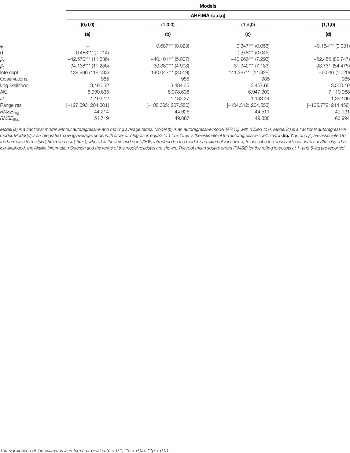
TABLE 1. Estimates of ARFIMA models with different orders where the response variable is the average daily radon measurements in Figure 1.
The results of the estimate models suggest that for all of them, the coefficients associated to the harmonic terms are significant, and the comparison with the models without the external covariates are worse (the results are not shown).
Examining the results of Models (a) and (c) where the parameter d is estimated varying in the real values, the fractional parameter for both models is between 0 and 1, thus allowing us to reject both the case of pure stationarity (I = 0) and the unit root model (I = 1). The estimated parameters are statistically significant at the 1% level and lie within the interval (0, 0.5). The confidence intervals for the estimated fractional-integration parameters are relatively narrow and always in the positive range of persistent long-memory.
The results show that Model (c) is the best model in terms of fitting since it has the lowest AIC and the shorter range of the residuals. For the RMSE at 1- and 5-lag forecast, Model (a) performs slightly better than Model (c); however, the fractional model has too simple parametrization, and it is not able to describe the autocorrelation dynamic in the data (see the residuals time series in Figure 3 and the diagnostics on the residuals Figures 4, 5).
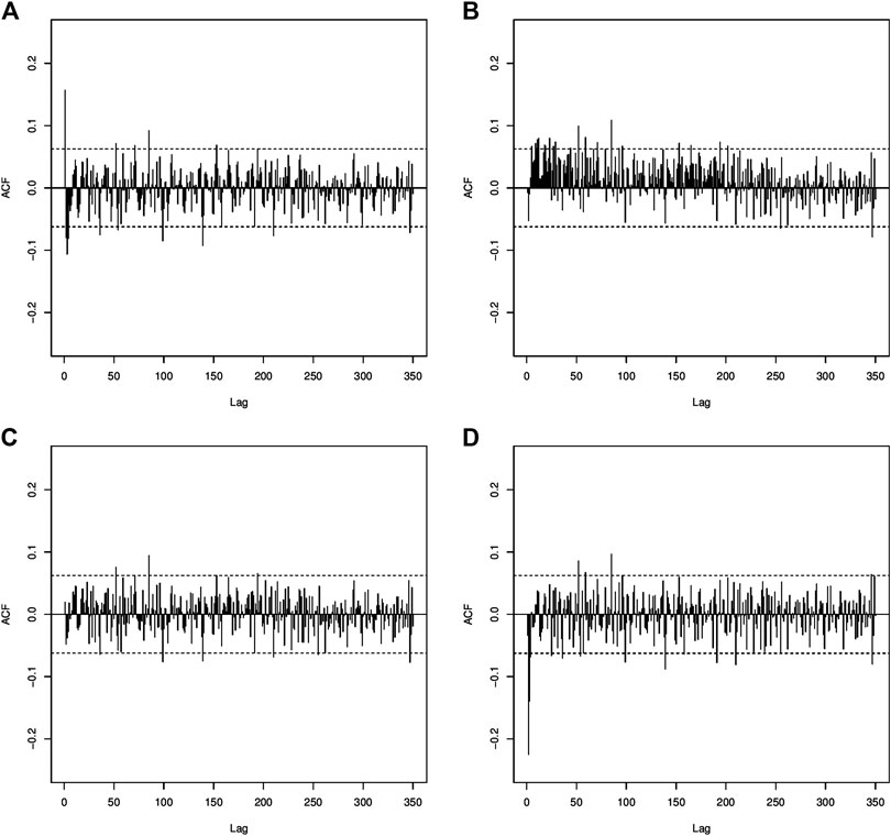
FIGURE 4. Autocorrelation coefficients of the residuals of the estimated Models (A–D) as labeled in Table 1. The horizontal lines indicate the confidence interval at 95% for not significant correlation coefficient.
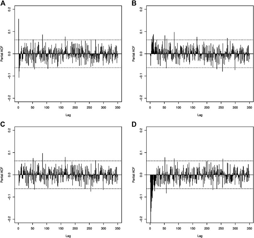
FIGURE 5. Partial autocorrelation coefficients of the estimated Models (A–D) as labeled in Table 1. The horizontal lines indicate the 95% confidence bounds for strict white noise.
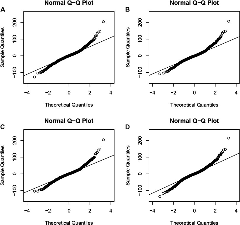
FIGURE 6. Q‐Q norm of the residuals time series for the estimated Models (A–D) as labeled in Table 1 to check the normality assumption.
For all the estimated models, the assumption of constant variability along time appears respected (Figure 3), and there is not a marked pattern in the residuals, in particular the seasonality behavior in the original data is not present (Figure 1). The residual ACF (Figure 4) and PACF (Figure 5) of the fitted Models (a), (b), and (d) show that there are significant estimated correlation coefficients at short lags; therefore, these models are not adequate. Instead, for the Model (c), the residual ACF and PACF are not significant. The Ljung–Box test from 1 to 10 lags is computed to assess the absence of serial autocorrelation in the residuals. For the model (c), the null hypothesis is not rejected for all the considered lags. The q-q plot of the residuals is used to assess the normality assumption of the considered models. In Figure 6, for all the four models, there is a slight departure from the normality in the tails. Finally, the plots of observed and estimated values obtained with the four model at 1- and 5-lags are shown in Figures 7, 8 respectively.
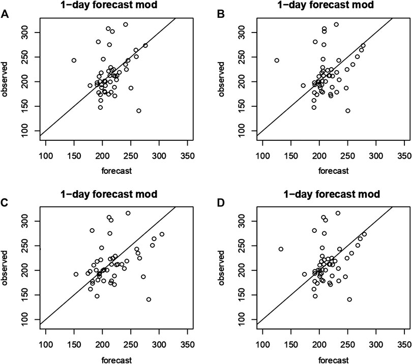
FIGURE 7. Prediction at 1‐lag and observed radon measurements for the estimated Models (A–D) as labeled in Table 1.
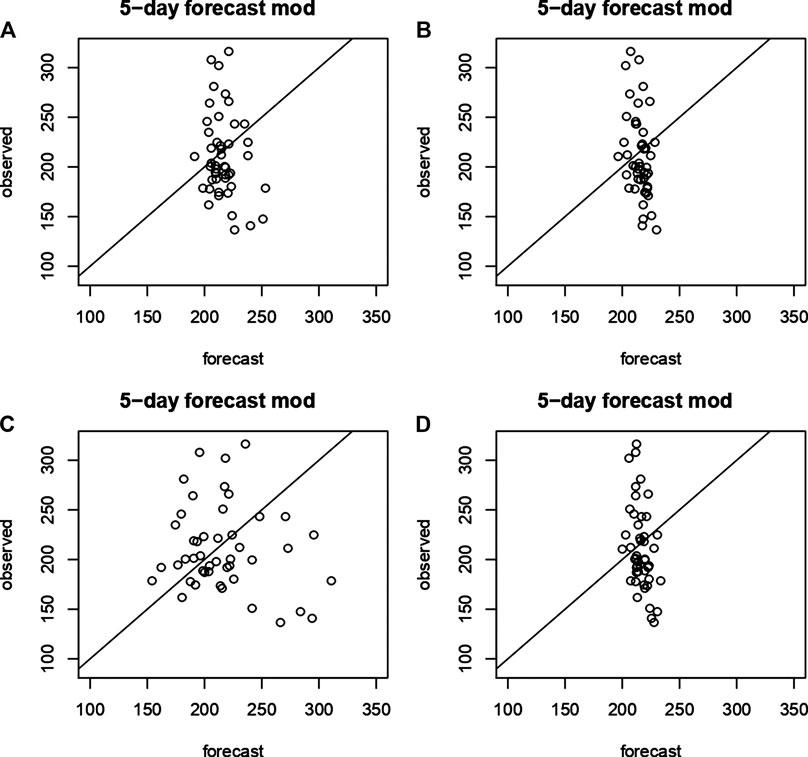
FIGURE 8. Prediction at 5‐lag and observed radon measurements for the estimated Models (A–D) as labeled in Table 1.
Being sensitive to crustal stress, the soil radon discharge is widely considered as a promising earthquake precursor. Because of the influence of several environmental factors and local geological conditions, pre-seismic radon anomalies cannot be easily detected with conventional statistical methodologies.
The general approach is to model the observation and highlight the anomalies. This study tests a radon concentration time series, covering almost 3 years, for the presence of nonstationarity (seasonality and trend) and long memory. Overall, our results indicate that the radon series are better characterized as being stationary in the trend, but with persistent long-memory and 1-year seasonality. It is widely accepted that the periodic annual component in radon concentration time series is correlated to the climatic variables as temperature, atmospheric pressure, and rainfall (Siino et al., 2019a; Siino et al., 2019b; D’Alessandro et al., 2020).
The class of the ARFIMA model presented here provides a general framework for representing radon time series that display both short- and long-term persistence. The analysis of daily radon shows that the ARFIMA approach provides a better representation of the observed data with respect to the traditional ARMA and ARIMA models. More specifically, according to the model comparison, an ARFIMA model with an autoregressive term has a better fitting to the data. The estimated fractional integration parameters of this ARFIMA model is positive and smaller than 0.5 (
The occurrence of long-range correlation in the time series has been also tested by the application of Detrended Fluctuation Analysis (DFA) (Höll et al., 2019). Also, this method indicates that the radon concentration can be considered as coming from a fractional Gaussian noise (fGn).
It is widely recognized that radon time series are strongly controlled by the combination between site-specific factors and large-scale variations (i.e., astronomical cycles) (Schery et al., 1984; Schumann et al., 1988; Aumento, 2002; Piersanti et al., 2015; Crockett et al., 2018). It is note worth that the proposed approach (based only on radon measurements) is able to describe with good reliability the data and also to perform short-term forecasts when accurate radon measurements are taken for a reasonably long time span.
Model residuals could be retrospectively compared with external evidence of transitory phenomena in the study area (seismic, meteorological, etc.). Having available the seismic catalogue of the area, we make an attempt to find the relationship between the found anomalies in the radon time series and the earthquakes. In this case study, there is no evidence between the residuals of the fitted model and the seismicity in the study area. However, it should be considered the absence of any relevant earthquakes during the observation period but only the occurrence of background seismicity. In fact, in spite of the well-known seismicity of the area, the larger recorded event was a
In conclusion, our findings on the long-memory nature of radon measurements have important implications that can be useful for further analysis. The long-memory structure is the result of a long-lasting and aperiodic process such as a weather episode and changes in the circulation of geofluids, ground sealing. However, at this stage (i.e., a single time series), it is not possible to propose a comprehensive physical/geological or physical/meteorological mechanism that could account for the long memory in radon concentration time series; moreover, it would also be out of the purpose of this work. The extension of this methodology by applying the ARFIMA models to longer radon time series, or to series with a different measurement range, or recorded in other monitoring sites, could provide the missing hints.
The proposed approach represents an effective tool to analyze radon signals, and in particular to detect long-range memory in the times series, which are the necessary preliminary steps to explore the relationship between radon anomalies and seismic activity. Finally, it would be interesting for further analysis, to compare the forecast of radon observations, or the identification of preseismic anomalies with those obtained with other methods such as the linear regression analysis (Stojanovska et al., 2017), the artificial neural network approach (Pasini and Ameli, 2003), or the decision tree method (Zhang et al., 2020). It would also be interesting to consider other external covariates in the model formulation Eq. 7, such as weather variables (Stránský and Thinová, 2017).
The raw data supporting the conclusions of this article will be made available by the authors, without undue reservation.
AD and MS conceived the idea of the analysis approach. Data analyses and comments were made by MS. MS and SS prepared and reviewed the manuscript.
The authors declare that the research was conducted in the absence of any commercial or financial relationships that could be construed as a potential conflict of interest.
We thank A. Piersanti e V. Cannelli (Istituto Nazionale di Geofisica e Vulcanologia) who provided the data.
Aumento, F. (2002). Radon tides on an active volcanic island: Terceira, azores. Geofisc. Int. 41, 499–505. doi:10.22201/IGEOF.00167169P.2002.41.4.501
Barbosa, S., Donner, R., and Steinitz, G. (2015). Radon applications in geosciences—progress and perspectives. Eur. Phys. J. Spec. Top. 224, 597–603. doi:10.1140/epjst/e2015-02393-y
Baskaran, M. (2016). Radon: a tracer for geological, geophysical and geochemical studies. New York, NY: Springer.
Baykut, S., Akgül, T., İnan, S., and Seyis, C. (2010). Observation and removal of daily quasi-periodic components in soil radon data. Radiat. Meas. 45, 872–879. doi:10.1016/j.radmeas.2010.04.002
Belbute, J. M., and Pereira, A. M. (2017). Do global co2 emissions from fossil-fuel consumption exhibit long memory? A fractional-integration analysis. Appl. Econ. 49, 4055–4070. doi:10.1080/00036846.2016.1273508
Bowers, M. C., and Tung, W.-w. (2018). Variability and confidence intervals for the mean of climate data with short-and long-range dependence. J. Clim. 31, 6135–6156. doi:10.1175/JCLI-D-17-0090.1
Box, G. E., Jenkins, G. M., Reinsel, G. C., and Ljung, G. M. (2015). Time series analysis: forecasting and control. Hoboken: John Wiley & Sons.
Cannelli, V., Piersanti, A., Galli, G., and Melini, D. (2018). Italian radon monitoring network (iron): a permanent network for near real-time monitoring of soil radon emission in Italy. Ann. Geophys. 61, 444. doi:10.4401/ag-7604
Clauset, A., Shalizi, C. R., and Newman, M. E. (2009). Power-law distributions in empirical data. SIAM Review. 51, 661–703. doi:10.1137/070710111
Conraria, L. A., and Soares, M. J. (2011). The continuous wavelet transform: a primer. NIPE Work. Paper. 16, 1–43. doi:10.1111/joes.12012
Crockett, R. G., Gillmore, G. K., Phillips, P. S., Denman, A. R., and Groves-Kirkby, C. J. (2006). Tidal synchronicity of built-environment radon levels in the UK. Geophys. Res. Lett. 33, 1319–1334. doi:10.1029/2005GL024950
Crockett, R. G., Groves-Kirkby, C. J., Denman, A. R., and Phillips, P. S. (2018). Significant annual and sub-annual cycles in indoor radon concentrations: seasonal variation and correction. Geol. Soc. Lond. Spl. Publ. 451, 35–47. doi:10.1144/SP451.2
Cuculeanu, V., Lupu, A., and Sütö, E. (1996). Fractal dimensions of the outdoor radon isotopes time series. Environ. Int. 22, 171–179. doi:10.3390/environments6030029
D’Alessandro, A., Scudero, S., Siino, M., Alessandro, G., and Mineo, R. (2020). Long-term monitoring and characterization of soil radon emission in a seismically active area. Geochem. Geophys. Geosyst. 21, e2020GC009061. doi:10.1029/2020GC009061
Dickey, D. A., and Fuller, W. A. (1979). Distribution of the estimators for autoregressive time series with a unit root. J. Am. Stat. Assoc. 74, 427–431. doi:10.1080/01621459.1979.10482531
Donner, R. V., Potirakis, S. M., Barbosa, S. M., Matos, J. A., Pereira, A. J., and Neves, L. J. (2015). Intrinsic vs. spurious long-range memory in high-frequency records of environmental radioactivity. Eur. Phys. J. Spec. Top. 224, 741–762. doi:10.1140/epjst/e2015-02404-1
Dunn, J., and Henschel, B. (1989). Statistical aspects of autoregressive-moving average models in the assessment of radon mitigation. Environ. Int. 15, 247–252. doi:10.16966/2576-6430.112
Höll, M., Kiyono, K., and Kantz, H. (2019). Theoretical foundation of detrending methods for fluctuation analysis such as detrended fluctuation analysis and detrending moving average. Phys. Rev. 99, 033305. doi:10.1103/PhysRevE.99.033305
Hosking, J. R. M. (1981). Fractional differencing. Biometrika 68, 165–176. doi:10.1093/biomet/68.1.165
Hurst, H., Black, R., and Simaika, Y. (1965). Long-term storage: an experimental study constable. London, UK: Constable.
Mandelbrot, B. B., and Wallis, J. R. (1968). Noah, joseph, and operational hydrology. Water Res. Res. 4, 909–918. doi:10.1029/WR004i005p00909
Mandelbrot, B. B., and Wallis, J. R. (1969). Robustness of the rescaled range r/s in the measurement of noncyclic long run statistical dependence. Water Resour. Res. 5, 967–988. doi:10.1029/WR005i005p00967
Montanari, A., Rosso, R., and Taqqu, M. S. (1997). Fractionally differenced arima models applied to hydrologic time series: identification, estimation, and simulation. Water Res. Res. 33, 1035–1044. doi:10.1029/97WR00043
Morales-Simfors, N., Wyss, R. A., and Bundschuh, J. (2019). Recent progress in radon-based monitoring as seismic and volcanic precursor: a critical review. Crit. Rev. Environ. Sci. Technol. 50, 1–34. doi:10.1080/10643389.2019.1642833
Nikolopoulos, D., Matsoukas, C., Yannakopoulos, P., Petraki, E., Cantzos, D., and Nomicos, C. (2018). Long-memory and fractal trends in variations of environmental radon in soil: results from measurements in lesvos island in Greece. J. Earth Sci. Clim. Chang. 9, 1–11. doi:10.4172/2157-7617.1000465
Pan, J.-N., and Chen, S.-T. (2008). Monitoring long-memory air quality data using arfima model. Environ. Off. J. Int. Environ. Soc. 19, 209–219. doi:10.1002/env.882
Papacharalampous, G., Tyralis, H., and Koutsoyiannis, D. (2018a). One-step ahead forecasting of geophysical processes within a purely statistical framework. Geosci. Lett. 5, 12. doi:10.1186/s40562-018-0111-1
Papacharalampous, G., Tyralis, H., and Koutsoyiannis, D. (2018b). Predictability of monthly temperature and precipitation using automatic time series forecasting methods. Acta Geophys. 66, 807–831. doi:10.1007/s11600-018-0120-7
Pasini, A., and Ameli, F. (2003). Radon short range forecasting through time series preprocessing and neural network modeling. Geophys. Res. Lett. 30, 39. doi:10.1029/2002GL016726
Piersanti, A., Cannelli, V., and Galli, G. (2015). Long term continuous radon monitoring in a seismically active area. Ann. Geophys. 58, 0437. doi:10.4401/ag-6735
Pinault, J.-L., and Baubron, J.-C. (1996). Signal processing of soil gas radon, atmospheric pressure, moisture, and soil temperature data: a new approach for radon concentration modeling. J. Geophys. Res.: Solid Earth. 101, 3157–3171. doi:10.1029/95JB03121
Reisen, V. A., Monte, E. Z., da Conceição Franco, G., Sgrancio, A. M., Molinares, F. A. F., Bondon, P., et al. (2018). Robust estimation of fractional seasonal processes: modeling and forecasting daily average so2 concentrations. Math. Comput. Simulat. 146, 27–43. doi:10.1016/j.matcom.2017.10.004
Roesch, A., and Schmidbauer, H. (2018). WaveletComp: computational wavelet analysis. R package version 1.1.
Schery, S., Gaeddert, D., and Wilkening, M. (1984). Factors affecting exhalation of radon from a gravelly sandy loam. J. Geophys. Res.: Atmos. 89, 7299–7309. doi:10.1029/JD089iD05p07299
Schumann, R., Owen, D., and Asher-Bolinder, S. (1988). “Factors affecting soil-gas radon concentrations at a single site in the semiarid western us,” in Proceedings of the 1988 EPA symposium on radon and radon reduction technology 2, Citeseer. Washington, DC, September 22–25, 1992.
Shumway, R. H., and Stoffer, D. S. (2017). Time series analysis and its applications: with R examples. New York, NY: Springer.
Siino, M., Alessandro, G., Buonmestieri, S., D’Alessandro, A., Mineo, R., and Scudero, S. (2019a). “Radon concentration in the ragusa province (sicily, Italy),” in International scientific conference man and Karst. Silicy, Italy, June 24–26, 2019.
Siino, M., Scudero, S., Cannelli, V., Piersanti, A., and D’Alessandro, A. (2019b). Multiple seasonality in soil radon time series. Sci. Rep. 9, 8610. doi:10.1038/s41598-019-44875-z
Stojanovska, Z., Ivanova, K., Bossew, P., Boev, B., Zora, S., Kolar, P., et al. (2017). Prediction of long-term in door radon concentration based on short-term measurements. Nucl. Technol. Radiat. 32, 77–84. doi:10.2298/NTRP1701077S
Stránský, V., and Thinová, L. (2017). Radon concentration time series modelling and application discussion. Radiat. Protect. Dosim. 177, 155–159. doi:10.1093/rpd/ncx207
Team, R. D. C. (2005). R: a language and environment for statistical computing. Vienna, Austria: R Foundation for Statistical Computing.
Toutain, J.-P., and Baubron, J.-C. (1999). Gas geochemistry and seismotectonics: a review. Tectonophysics 304, 1–27. doi:10.1016/S0040-1951(98)00295-9
Udovičić, V., Filipović, J., Dragić, A., Banjanac, R., Joković, D., Maletić, D., et al. (2014). Daily and seasonal radon variability in the underground low-background laboratory in belgrade, Serbia. Radiat. Protect. Dosim. 160, 62–64. doi:10.1093/rpd/ncu109
Veenstra, J. Q. (2013). Persistence and anti-persistence: theory and software. PhD thesis. Ontario (Canada): The University of Western Ontario.
Wang, W., Van Gelder, P., Vrijling, J., and Chen, X. (2007). Detecting long-memory: Monte Carlo simulations and application to daily streamflow processes. Hydrol. Earth Syst. Sci. Discuss. 11, 851–862. doi:10.5194/hessd-3-1603-2006
Woith, H. (2015). Radon earthquake precursor: a short review. Eur. Phys. J. Spec. Top. 224, 611–627. doi:10.1140/epjst/e2015-02395-9
Yan, R., Woith, H., Wang, R., and Wang, G. (2017). Decadal radon cycles in a hot spring. Sci. Rep. 7, 12120. doi:10.1038/s41598-017-12441-0
Yaya, O. S., and Fashae, O. A. (2015). Seasonal fractional integrated time series models for rainfall data in Nigeria. Theor. Appl. Climatol. 120, 99–108. doi:10.1007/s00704-014-1153-8
Keywords: autoregressive integrated moving average model, autoregressive fractionally integrated moving average model, continuous wavelet transform, radon, spectral analysis, forecast
Citation: Siino M, Scudero S and D’Alessandro A (2020) Stochastic Models for Radon Daily Time Series: Seasonality, Stationarity, and Long-Range Dependence Detection. Front. Earth Sci. 8:575001. doi: 10.3389/feart.2020.575001
Received: 23 June 2020; Accepted: 22 September 2020;
Published: 10 November 2020.
Edited by:
Francesco Italiano, National Institute of Geophysics and Volcanology, ItalyReviewed by:
Kit Lai, Universiti Brunei Darussalam, BruneiCopyright © 2020 Siino, Scudero and D'Alessandro. This is an open-access article distributed under the terms of the Creative Commons Attribution License (CC BY). The use, distribution or reproduction in other forums is permitted, provided the original author(s) and the copyright owner(s) are credited and that the original publication in this journal is cited, in accordance with accepted academic practice. No use, distribution or reproduction is permitted which does not comply with these terms.
*Correspondence: Salvatore Scudero, c2FsdmF0b3JlLnNjdWRlcm9AaW5ndi5pdA==
Disclaimer: All claims expressed in this article are solely those of the authors and do not necessarily represent those of their affiliated organizations, or those of the publisher, the editors and the reviewers. Any product that may be evaluated in this article or claim that may be made by its manufacturer is not guaranteed or endorsed by the publisher.
Research integrity at Frontiers

Learn more about the work of our research integrity team to safeguard the quality of each article we publish.