Comparison of Different Methods for Spatial Downscaling of GPM IMERG V06B Satellite Precipitation Product Over a Typical Arid to Semi-Arid Area

Spatial downscaling is an effective way to obtain precipitation with sufficient spatial details. The performance of downscaling is typically determined by the empirical statistical relationships between precipitation and the used auxiliary variables. In this study, we conducted a comprehensive comparison of five empirical statistical methods for spatial downscaling of GPM IMERG V06B monthly and annual precipitation with a relatively long time series from 2001 to 2015 over a typical semi-arid to arid area (Gansu province, China). These methods included two parametric regression methods (univariate regression, or UR; multivariate regression, or MR) and three machine learning methods (artificial neural network, or ANN; support vector machine, or SVM; random forests, or RF), which were used to downscale the satellite precipitation from 0.1° (∼10 km) to 1 km spatial resolution. Five commonly used indices which were normalized differential vegetation index (NDVI), elevation, land surface temperature (LST), and latitude and longitude were selected as auxiliary variables. The downscaled results were validated using a total of 80 rain gauge station data during 2001–2015. Results showed that latitude had the overall largest correlation with IMERG annual precipitation, also evidenced by feature importance measurements in RF. The downscaled results at monthly scale were overall consistent with the results at annual scale. The machine learning-based methods had better predictive ability of the original IMERG precipitation than parametric regression methods, with larger coefficient of determination (R²) and smaller root-mean-square error (RMSE) as well as relative root-mean-square error (RRMSE). The downscaled 1 km IMERG precipitation by parametric regression methods had obvious underestimations (positive residual errors) in the south and east of Gansu province and overestimations (negative residual errors) in the west. In addition, the validation results of parametric regression downscaling methods showed large improvements after residual correction, while the improvements were small in the machine learning-based methods. However, the interpolation algorithm included in residual correction can cause certain errors in the downscaled results due to the ignorance of precipitation spatial heterogeneity. The machine learning-based RF downscaling had the smallest residual errors and the overall best validation results, showing great potentials to provide accurate precipitation with high spatial resolution.

Introduction

Precipitation is a key variable in hydrological cycle and climate change, and the grid-based precipitation with finer spatiotemporal resolution and high accuracy is essential for hydrological, meteorological, and climatology research in local basins and regions (Duan and Bastiaanssen, 2013; Liu et al., 2016; Ma et al., 2020). Traditional rain gauge-based ground observations are sparse in space, especially over the remote mountainous areas. Satellite-based precipitation has the advantages of complete coverage and convenient access to the data, which is an effective way to obtain precipitation at a regional or global scale (Kidd and Levizzani, 2011). The research on satellite precipitation has received increasing interests, and various satellite precipitation estimates have been produced, such as Global Satellite Mapping Precipitation (GSMaP) (Kubota et al., 2007), Precipitation Estimation from Remote Sensing Information using Artificial Neural Network-Climate Data Record (PERSIANN-CDR) (Ashouri et al., 2015), Tropical Rainfall Measurement Mission (TRMM) Multisatellite Precipitation Analysis (TMPA) (Huffman et al., 2007), and IMERG [Integrated Multi-satellitE Retrievals for Global Precipitation Measurement (GPM)] (Hou et al., 2014). However, the relatively low spatial resolutions (e.g., 0.1°–0.5°) of the existing satellite precipitation products are too coarse for hydrological simulation at the catchment scales.

Spatial downscaling techniques provide an effective way to bridge the spatial scale gap between the low/coarse resolution and the high/fine resolution. There are two major categories of downscaling techniques: statistical downscaling and dynamical downscaling (Sachindra and Perera, 2016). The dynamic downscaling is based on the mathematical representations of the complex physical process of atmosphere, ocean, and land surface, which limits its applicability due to the intensive computational cost and the requirement of huge volume data (Wilby and Wigley, 2000; Sachindra and Perera, 2016). Instead, statistical downscaling depends on the empirical statistical relationships between object variable and auxiliary variables, which is of high efficiency and has been widely used for satellite precipitation downscaling in recent studies (Duan and Bastiaanssen, 2013; Jia et al., 2011; Chen et al., 2015; Shi et al., 2015; Ma et al., 2018; Sharifi et al., 2019).

The performance of statistical downscaling is typically influenced by their auxiliary variable(s) and the empirical statistical relationships. At present, most satellite precipitation downscaling studies are conducted by selecting the auxiliary variables that have high correlation with precipitation. The normalized differential vegetation index (NDVI) is the most widely used auxiliary variable because of the close NDVI-precipitation relationship (Foody et al., 2003), especially in arid and semi-arid regions where the growth of vegetation is mainly fed by precipitation. By establishing the statistical relationship between NDVI and TMPA satellite precipitation at a coarse resolution of 0.25° (∼25 km), the accurate 1 km precipitation was obtained using the statistical downscaling method (Immerzeel et al., 2009; Duan and Bastiaanssen, 2013). The elevation-precipitation relationship also varies spatially, and thus the introduction of elevation in the downscaling method can better predict the precipitation distribution in the areas with complex terrain (Jia et al., 2013). However, the relationship between precipitation and land surface characteristics (NDVI, elevation, geographical location, and so on) is spatially nonstationary. Therefore, the representation of precipitation spatial variability by NDVI-precipitation relationship or elevation-precipitation relationship alone is insufficient (Xu et al., 2015). Fang et al. (2013) found that precipitation is also affected by the geographic location (latitude and longitude). Chen et al. (2015) firstly introduced the Moderate Resolution Imaging Spectroradiometer (MODIS) land surface temperature (LST) to improve the downscaling results for TMPA precipitation over an arid to semi-arid area. It has also been found by Jing et al. (2016) and López et al. (2018) that LST and slope as well as aspect had significant influences on satellite precipitation downscaling. On the whole, the inclusion of auxiliary variables from single one to multiple ones can better describe the complicated relationships between precipitation and land surface characteristics.

In addition to auxiliary variable, the empirical statistical relationship between satellite precipitation and the used auxiliary variables can also affect the downscaling results. Several empirical statistical relationships have been developed in downscaling models, including univariate regression (UR) (Immerzeel et al., 2009; Duan and Bastiaanssen, 2013), multivariate regression (MR) (Jia et al., 2013), and geographically weighted regression (GWR) (Chen et al., 2015; Xu et al., 2015; Zhao et al., 2017). However, these parametric regression-based methods are difficult to reflect the spatial heterogeneity between precipitation and land surface characteristics (e.g., NDVI, LST, and elevation). With the development of artificial intelligence algorithms, many machine learning algorithms, such as artificial neural network (ANN), support vector machine (SVM), random forests (RF), and deep learning, have been proposed to solve the nonlinear problems. Shi et al. (2015) have developed a RF-based downscaling method to obtain the 1 km TMPA data. Similar studies have been also reported by Jing et al. (2016) and Retalis et al. (2017). However, the current studies on spatial downscaling of satellite precipitation focus mainly on the TRMM-era precipitation, and the downscaling studies on GPM-era precipitation are relatively few. It is worth emphasizing that TRMM mission came to an end on June 2015.

As the successor of TRMM, GPM opens a new era of satellite precipitation measurements, providing more detailed precipitation information with a 0.1° (∼10 km) spatial resolution since March 2014 (Chen et al., 2018). In particular, the latest released post-real-time Level-3 GPM IMERG Final Run product (IMERG V06B) in June 2019 provides more accurate precipitation estimates with a relatively long time series (June 2000 to the present), compared to the previous versions. To the best of our knowledge, only few researchers have attempted to downscale the GPM-era precipitation. Ma et al. (2018) have compared the downscaled 1 km IMERG V05B and TMPA data in 2015 using the RF method and showed that downscaled results based on IMERG V05B performed better than those based on TMPA. Sharifi et al. (2019) have adopted the ANN method for the downscaling of IMERG V05B precipitation data in 2015. However, these spatial downscaling studies use only short-term rainfall data (1 year) and lack a comprehensive comparison of the downscaling performances of different empirical statistical methods, especially the machine learning-based methods.

To fill the research gaps, this study conducted a comprehensive comparison on the empirical statistical methods for spatial downscaling of the IMERG V06B monthly and annual precipitation from 2001 to 2015. A typical arid to semi-arid region in China (Gansu province) was selected as the study area. Five commonly used indices (i.e., NDVI, elevation, LST, latitude, and longitude) were selected as auxiliary variables. Two parametric regression methods (UR and MR) and three machine learning-based nonparametric regression methods (ANN, SVM, and RF) were compared to demonstrate their robustness. The downscaled results with and without residual correction were also compared and validated using a total of 80 rain gauge stations over the study area.

Study Area and Datasets

Study Area

Gansu province is a typical arid to semi-arid region, which is located in northwestern China (N 32°31′–42°57′, E 92°13′–108°46′) and covers a total land area of 4.26 × 10⁵ km² (Figure 1). The terrain of Gansu province is very complex and inclines from southwest to northeast. Due to the effect of the terrain and the geographical location, the precipitation spatial distribution shows a pattern of decreasing from southeast to northwest (Chen et al., 2015). The annual precipitation is about 700–800 mm in the southeast of Gansu province, while the annual precipitation in the northwest is only about 40–200 mm. Precipitation is mainly concentrated in summer months (May–September). Bare land and grass are the two main land cover types of Gansu province, accounting for 82.4% of the total area (Figure 1). The bare land is mainly distributed in the northwest of Gansu province. The forest and arable land are distributed in the southeast of Gansu province, where the climate is humid to semi-humid and precipitation is relatively high.

FIGURE 1

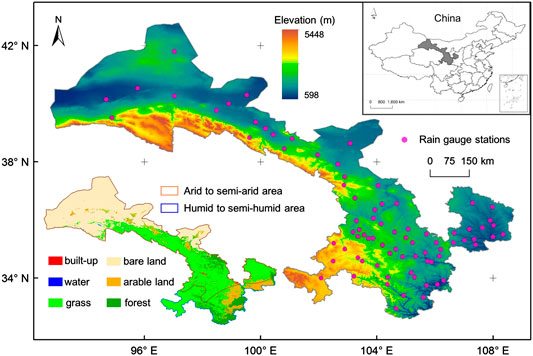
FIGURE 1. Location of Gansu province and rain gauge stations. The elevation, climate zones, and land cover types are also presented.

Datasets

Rain Gauge Data

A total of 80 rain gauges from 2001 to 2015 in Gansu province were used as the ground reference values for validation in this study. The rain gauges were obtained from the China Meteorological Administration, which provides high-quality information of daily precipitation records from stations over China since 1951 (Shen et al., 2010). The spatial distribution of the rain gauge stations is uneven, with dense sites in the southeast and sparse sites in the northwest (Figure 1). The daily rainfall in each month/year was accumulated to obtain the monthly/annual rainfall.

GPM IMERG V06B

The GPM mission is initiated by the Japan Aerospace Exploration Agency (JAXA) and the United States National Aeronautics and Space Administration (NASA), which is an international constellation of satellites and consists of one Core Observatory satellite and also ten partner satellites (Lu et al., 2018) that provide the next-generation global precipitation measurement. Compared to the TRMM, a key advancement of GPM is the extended capability to detect light rain (<0.5 mm/h) and solid rain by carrying the first space-borne Ku (13 GHz) and Ka (35 GHz) bands Dual-frequency Precipitation Radar (DPR) and a multichannel (10–183 GHz) GPM Microwave Imager (GMI) (Hou et al., 2014). IMERG is the level 3 multi-satellite precipitation algorithm of GPM, which is designed to combine all microwave estimates of the GPM constellation, infrared estimates, and precipitation gauge analyses to build a long record of global uniformly gridded precipitation products over time and space. The latest released IMERG V06B product provides half-hourly and monthly satellite precipitation estimates at a 0.1° (∼10 km) spatial resolution over the globe with a relatively long time series (June 2000 to the present, delayed by about 3.5 months). The monthly GPM IMERG V06B (abbreviated as IMERG) data from 2001 to 2015 was used in this study, which was downloaded at the website: https://gpm1.gesdisc.eosdis.nasa.gov/data/GPM_L3/GPM_3IMERGM.06/. The monthly precipitation was aggregated to obtain the IMERG annual precipitation.

Système Pour l’Observation de la Terre Normalized Differential Vegetation Index

The Système Pour l’Observation de la Terre (SPOT) VEGETATION (VGT) NDVI data at 1 km spatial resolution were used in the study. The VGT-S (synthesis) products provide daily NDVI product (VGT-S1) and 10-day synthesis NDVI product (VGT-S10) using the maximum value composite (MVC) method (Maisongrande et al., 2004). The geometric, radiometric, and atmospheric corrections have been conducted in the data preprocessing procedures. The VGT-S10 NDVI products from 2001 to 2015 were obtained in this study from http://www.vito-eodata.be/collections/srv/eng/main.home. The monthly/annual NDVI data were calculated by averaging the VGT–S10 NDVI data in a given month/year. The monthly/annual NDVI data with a spatial resolution of 1 km were aggregated to 10 km by using pixel averaging for the application purpose of spatial downscaling.

MODIS LST

The Terra-MODIS LST data used in the study is the MOD11A2 product, which provides an average 8-day per-pixel LST data at 1 km spatial resolution. The MOD11A2 product is composed using the MVC method to eliminate the influence of cloud (Wan, 2008). The 8-day composed MODIS LST data from 2001 to 2015 were downloaded from the USGS website (https://e4ftl01.cr.usgs.gov/MOLT/MOD11A2.006//). The monthly/annual LST data were calculated by averaging the 8-day LST data in a given month/year, and the 1 km monthly/annual LST data were aggregated to 10 km by using pixel averaging.

Elevation and Geographic Location

The elevation data used in this study were from the Shuttle Radar Topography Mission digital elevation model with a spatial resolution of 90 m, which is available from the public website at https://dds.cr.usgs.gov/srtm/version2_1/SRTM30/ (Rodriguez et al., 2006). The elevation data at 90 m resolution were aggregated to 1 and 10 km by using pixel averaging, respectively. The latitude and longitude data at 1 and 10 km resolutions were also extracted from the elevation data in this study.

Methodology

General Statistical Spatial Downscaling Procedure

The general procedure of the statistical spatial downscaling is to establish the empirical statistical relationship between the object variable and the corresponding auxiliary variables at low/coarse spatial resolution. The empirical statistical relationship is considered to be also applicable at high/fine spatial resolution. Then, the established empirical statistical relationship is applied to the auxiliary variables at the fine spatial resolution for obtaining the downscaled object variable at fine spatial resolution. The flowchart of the general downscaling procedure is shown in Figure 2.

FIGURE 2

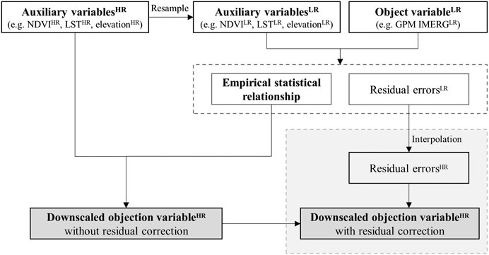
FIGURE 2. Flowchart of the general statistical spatial downscaling procedure. The superscripts HR and LR refer to the high/fine resolution and the low/coarse resolution, respectively.

In this study, the object variable was the IMERG monthly/annual satellite precipitation data which was downscaled from 10 to 1 km resolution and was validated by 80 rain gauge data in the study area. Five commonly used auxiliary variables (i.e., NDVI, elevation, LST, latitude, and longitude) were selected according to the previous study of Chen et al. (2015). The specific steps are described as follows.

(1) The auxiliary variables (i.e., NDVI, elevation, LST, latitude, and longitude) at 1 km spatial resolution were resampled to 10 km using the pixel averaging method. The outliers of NDVI pixels (the snow and the water body pixels) were eliminated by the threshold (NDVI < 0) (Jing et al., 2016).

(2) Two parametric regression models (UR and MR) and three machine learning-based nonparametric regression models (ANN, SVM, and RF) were established between IMERG precipitation and five auxiliary variables (i.e., NDVI, elevation, LST, latitude, and longitude) at 10 km resolution. The residual errors, which mean the part of the precipitation cannot be explained by the auxiliary factors, were also calculated at 10 km resolution.

(3) The IMERG precipitation results without residual correction at 1 km resolution of different downscaling methods were obtained by the auxiliary variables at 1 km resolution and the established empirical statistical relationship.

(4) The spline interpolation method (Immerzeel et al., 2009; Duan and Bastiaanssen, 2013) was used to interpolate the residual errors at the spatial resolution of 10 km into 1 km. Then, the downscaled results with residual correction at 1 km resolution could be obtained by adding the interpolated residual errors to the downscaled results without residual correction.

Random Forests

RF is a nonparametric statistical “ensemble learning” method for classification and regression proposed by Breiman (2001). The RF algorithm combines a lot of tree predictors in which each tree depends on the value of independent sampling random vector and has the same distribution in the forest (Breiman, 2001). As an extension of the Classification and Regression Trees (CART), RF is designed to overcome the problem of over-fitting by introducing randomness into the individual regression trees and averaging a large collection of these de-correlated individual trees. There are two main parameters (the number of trees, ntree; the number of variables in the random subset at each node, mtry) in the RF algorithm, making it user-friendly (Liaw and Wiener, 2002). The main steps for implementing the RF algorithm are as follows:

(1) The ntree samples are selected using a bootstrap sample that contains two-thirds of the training data. The remaining one-third of the training data referred to the out-of-bag data (OOB sample) are left out of the bootstrap sample.

(2) The unpruned regression tree is grown to this sample. For each node, the mtry random subset of the variables (tree predictors) is selected at random and the best variables of the mtry variables are chosen to split the data.

(3) The new samples can be predicted by averaging the predictions of the ntree trees. In the training process, the OOB samples are used to estimate the prediction error:

$P=\frac{1}{N}{\displaystyle \sum _{i=1}^N{P}_i\left(t\right)},(1)$

where N represents the number of trees and $P_i\left(t\right)$ represents the prediction of each regression tree. It is noted that RF can provide the estimation of feature/variable importance by comparing the changes of OOB error when the specific variable is randomly permuted and other variables keep unchanged. In this study, the Matlab tools for the RF model (Windows-Precompiled-RF_Mexstandalone-v0.02toolbox) were used; it can be freely downloaded from https://code.google.com/archive/p/randomforest-matlab/downloads.

Support Vector Machine

SVM is a machine learning technique based on the VapnikChervonenkis (VC) dimension of statistical learning theory (Chang and Lin, 2011), which can capture the nonlinear relationship and thus perform better than conventional parametric regression. SVM was first developed by Vapnik (1995) for solving the classification problems and had been mainly used for regression and classification problems with small-and high-dimensional samples. The SVM regression uses a nonlinear mapping to map the input x into a high-dimensional feature space, so that the original nonlinear problem can be transformed into a linearly separable problem. A linear model is then constructed in this high-dimensional space. The linear model can be expressed as

$f\left(\text{x}\right)=\langle \mathrm{w}\cdot \Phi \left(\mathrm{x}\right)\rangle +b,(2)$

where $\Phi$ represents a high-dimensional feature space, which is nonlinearly mapped from the input space; b is the bias; and w is the weight vector. The kernel function is applied to avoid the disaster of dimension without increasing the complexity of calculation.

The libsvm developed by Chang and Lin (2011) is currently one of the most widely used SVM software (Song et al., 2012). Thus, the version 3.24 libsvm tools of the Matlab code were used in this study, which can be freely downloaded from http://www.csie.ntu.edu.tw/∼cjlin/libsvm. The important parameters in the libsvm include the kernel function, gamma in kernel function, and capacity parameter cost.

Artificial Neural Network

ANN is a statistical learning algorithm used in machine learning. It has been proposed more than half a century ago and has been successfully applied for downscaling purpose in several fields (Nourani et al., 2018). ANN has a strong ability to deal with nonlinear problems, and it is widely used to model the nonlinear relationships between object variable and auxiliary variables at different scales. ANN has three layers: an input layer, output layer, and one or more hidden layers. The neurons are the basic processing elements in ANN, and the weights are connections between neurons. Neural networks provide a learning rule to modify their weights and neurons based on input/output data. The general function of the ANN can be expressed as

$y=f\left({\displaystyle \sum _{i=1}^n{x}_i{w}_i-\theta }\right),(3)$

where y is the output layer; x_i is the input of the ith neuron; w_i is the weight of the ith neuron; f is the activation function; and $\theta$ is the threshold.

In this study, the backpropagation training algorithm (BP) (Sharifi et al., 2019), which has a three-layer network and has been integrated in Matlab tools, was used to train the network between the IMERG precipitation data and the auxiliary variables. The nonlinear sigmoid activation function was applied to hidden layers as well as output layers of the neural network. More details about BP neural network can be found in Retalis et al. (2017) and Sharifi et al. (2019).

Univariate Regression and Multivariate Regression

The UR and MR methods have been widely used to downscale the satellite precipitation in many previous studies (Immerzeel et al., 2009; Jia et al., 2013). In the UR method (Eq. 4), only one auxiliary variable which has a large correlation with IMERG precipitation was adopted to construct the regression relationship. Then, various regression methods (e.g., linear regression, exponential regression, logarithm regression, and polynomial regression) were compared to choose the best one (Chen et al., 2015):

$P^{UR}=a+bX+\epsilon ,(4)$

where P^UR represents the IMERG precipitation data in the UR method; a is the intercept of the auxiliary variable; b is the slope of the auxiliary variable (e.g., NDVI and latitude in this study); and $\epsilon$ represents the residual error.

In the MR method (Eq. 5), five auxiliary variables (i.e., NDVI, elevation, LST, latitude, and longitude) were used in this study. The formula of MR can be expressed as follows:

$P^{MR}=a+{\displaystyle \sum _{i=1}^5{b}_i{X}_i}+\epsilon ,(5)$

where P^MR represents the IMERG precipitation data in the MR method; X_i represents the ith auxiliary variable (i.e., NDVI, elevation, LST, latitude, and longitude in this study); and b_i is the ith slope of the auxiliary variables used in the MR method. It was noted that before the establishment of the statistical relationships in the MR downscaling method, logarithmic transformation of the input variables had been conducted to avoid the influence of variable skewness distribution. The stepwise regression method was also used in the MR method to define which auxiliary variables are useful and to find the strongest relationship between auxiliary variables and object variable (Lu et al., 2018).

Validation

Several commonly used validation indicators, including the spearman correlation coefficient (ρ), coefficient of determination (R²), root-mean-square error (RMSE), and relative root-mean-square error (RRMSE), were selected to evaluate the spatial downscaling performance of the GPM IMERG V06B monthly and annual precipitation. To validate the downscaling results with rain gauge data, the rain gauge station at the grid scale was extracted and matched to the nearest satellite pixel of the downscaled GPM IMERG V06B precipitation data using the nearest neighbor method (Ma et al., 2016; Chen et al., 2020).

Results

Model Performances of Different Downscaling Methods at Annual Scale

Table 1 shows the mean R² of the regression analysis results between annual GPM IMERG V06B satellite precipitation and five commonly used auxiliary variables (i.e., NDVI, elevation, LST, latitude, and longitude) from 2001 to 2015. In the UR method, the linear regression between satellite precipitation and auxiliary variables was conducted from 2001 to 2015, and the variables with the best correlation with GPM IMERG V06B precipitation were considered as the auxiliary variables. Then, various regression methods (e.g., linear regression, exponential regression, logarithm regression, and polynomial regression) were compared to choose the best regression method. It could be seen that latitude had the largest mean R² (0.861) with IMERG annual precipitation and NDVI had the second largest R² (0.806), while there was no significant correlation between elevation and IMERG annual precipitation in the study area. Therefore, both of NDVI and latitude were finally selected to establish the regression function in the UR method, and the two UR downscaling methods were named UR-NDVI and UR-Lat, respectively. The linear regression was finally selected in the UR method because of the largest result of R² among various regression methods in this study. In the MR method, all five auxiliary variables were adopted to construct the multiple linear regression function for downscaling the IMERG annual precipitation. The stepwise regression results from 2001 to 2015 showed that NDVI and latitude are useful auxiliary variables in the MR method (results are not shown for conciseness). Table 2 shows the parameter sets for three machine learning-based downscaling methods (ANN, SVM, and RF). The optimal parameters for three machine learning-based methods were obtained by a grid search algorithm, and the parameter sets with the best training result were selected. The input variables and output variable were normalized to between 0 and 1 in three machine learning-based downscaling methods before the establishment of the training models.

TABLE 1

TABLE 1. Regression analysis results between annual GPM IMERG V06B satellite precipitation and auxiliary variables from 2001 to 2015.

TABLE 2

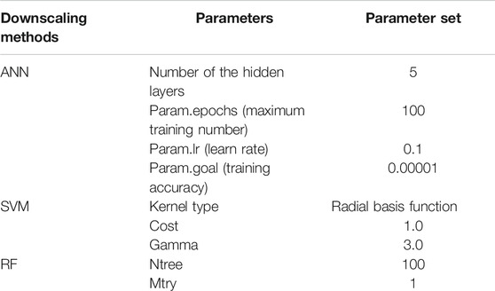
TABLE 2. Parameter settings for three machine learning-based downscaling methods.

Figure 3 presents the evaluation results of different downscaling methods using the original 10 km GPM IMERG V06B data at each year from 2001 to 2015. The R² results by different downscaling methods showed a similarity from 2001 to 2015. The RF downscaling method had the largest R², while the UR-NDVI method had the smallest R². The R² results of the ANN and SVM downscaling methods were very close. As a whole, the performances of R² of different methods were in the order UR-NDVI (worst, R² = 0.805) < UR-Lat (R² = 0.860) < MR (R² = 0.921) < ANN (R² = 0.978) < SVM (R² = 0.984) < RF (best, R² = 0.996). In terms of RRMSE and RMSE, they showed similar results with RF having lowest values and UR-NDVI having largest values. Table 3 shows the mean evaluation results from 2001 to 2015 of different downscaling methods, compared to the original GPM IMERG V06B precipitation data. The mean R² was 0.805 in the UR-NDVI method, but the mean R² was greatly improved in the RF method (0.996). The RF downscaling method also had the smallest mean RRMSE (0.044) and mean RMSE (13.407 mm), compared to the other downscaling methods, demonstrating the best prediction capability of IMERG annual precipitation spatial variation.

FIGURE 3

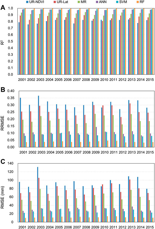
FIGURE 3. Evaluation results of different downscaling methods using the original GPM IMERG V06B data at each year from 2001 to 2015 (A-C) R2, RRMSE, and RMSE.

TABLE 3

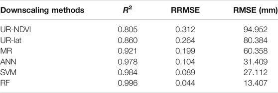
TABLE 3. Mean evaluation metrics of different downscaling methods using the original GPM IMERG V06B precipitation data.

Figures 4A,B present the mean feature importance from 2001 to 2015 and feature importance for each year in the RF downscaling method, respectively. The variables of NDVI, latitude, and longitude had relatively large values of mean feature importance in Figure 4A, of which the mean feature importance of latitude was the largest. Elevation had the smallest mean feature importance among the five auxiliary variables. It was noted that the feature importance of different variables were changing at different years. For example, the most important feature was latitude in 2004, whereas it was NDVI in 2006.

FIGURE 4

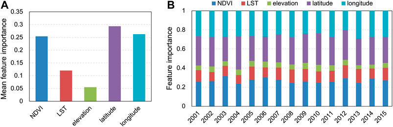
FIGURE 4. Feature importance in the RF downscaling method: (A) mean feature importance; (B) feature importance for each year.

Downscaled Results of Different Downscaling Methods at Annual Scale

Figures 5A–F show the downscaled IMERG precipitation at 1 km resolution without residual correction in 2015 by UR-NDVI, UR-Lat, MR, ANN, SVM, and RF. Figure 5G shows the spatial distribution of the original 10 km GPM IMERG V06B precipitation data in 2015. Since the GPM Core Observatory was launched on February 27, 2014, the IMERG data in 2015 can better represent the GPM-era precipitation. Therefore, the year of 2015 was selected for qualitative comparison. It could be seen that precipitation decreases from the southeast to the northwest, which is related to the humid and arid climatic zones. The white pixels in the downscaled results represent the outliers, including the extreme values caused by over-fitting and the blank values caused by the negative NDVI values. The downscaled IMERG precipitation could provide more detailed information due to the fine resolution (1 km) when compared with the original 10 km IMERG satellite precipitation data. However, the downscaled 1 km IMERG precipitation by UR-NDVI showed a larger spatial variability in Gansu province, which significantly overestimated the precipitation in region A and underestimated the precipitation in region C. The downscaled 1 km precipitation by UR-Lat had a smooth spatial continuity, which overestimated precipitation in region B and had an overfitting in the north of Gansu province. Since both of NDVI and latitude were adopted in the MR downscaling method, the precipitation distribution by MR presented a combination performance of two UR-based downscaling methods. Compared to the above parametric regression based methods, three machine learning-based nonparametric regression methods (ANN, SVM, and RF) had better applicability to capture precipitation distribution. Three machine learning downscaling methods had overall similar results in regions A, B, and C. In particular, the RF downscaling method could capture precipitation spatial heterogeneity well, especially in region A.

FIGURE 5

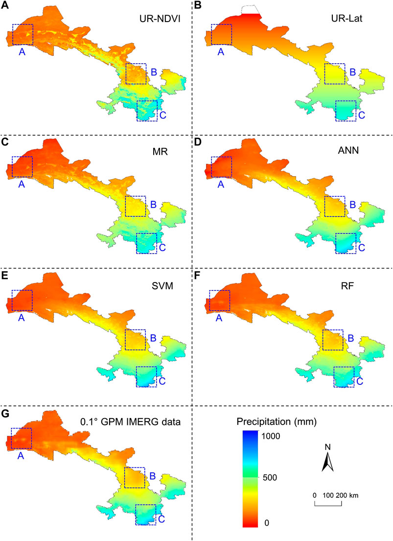
FIGURE 5. (A–F) Downscaled 1 km IMERG precipitation without residual correction in 2015 by UR-NDVI, UR-Lat, MR, ANN, SVM, and RF; (G) original 10 km GPM IMERG data in 2015.

Figures 6A–F show the spatial distribution of the interpolated residual errors at 1 km spatial resolution in 2015 by UR-NDVI, UR-Lat, MR, ANN, SVM, and RF. The positive residual errors represent that precipitation is underestimated by the auxiliary variables, while the negative residual errors mean the overestimation. The large positive residual errors in the south and east of Gansu province by UR-NDVI, UR-Lat and MR showed the underestimation in these regions, while the large absolute residual errors (negative values) in region B by UR-Lat and MR and in region A by UR-NDVI, UR-Lat, and MR showed the overestimation. Three machine learning-based downscaling methods had small absolute residual errors, of which the RF downscaling method had the smallest absolute residual errors. Table 4 shows the statistical results of spearman correlation coefficient (ρ) between auxiliary variables and residual errors of different downscaling methods in 2015. Overall, the statistical results of ρ between residual errors and different auxiliary variables in the MR, ANN, SVM, and RF downscaling models were very small. The residual errors in UR-NDVI decrease as latitude increases (ρ = −0.392) and increase as longitude increases (ρ = 0.458), while the residual errors in UR-Lat decrease as LST increases (ρ = −0.340).

FIGURE 6

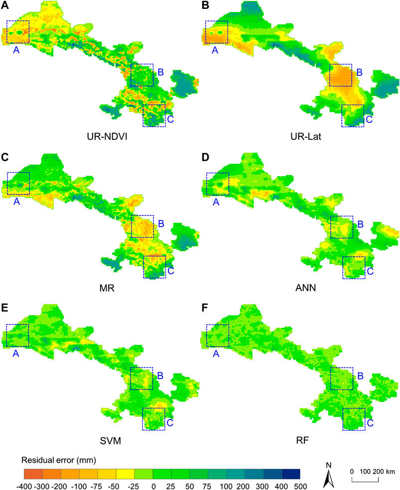
FIGURE 6. Interpolated residual errors at 1 km spatial resolution in 2015: (A–F) UR-NDVI, UR-Lat, MR, ANN, SVM, and RF.

TABLE 4

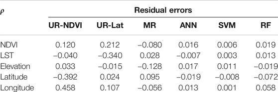
TABLE 4. Statistical results of Spearman correlation coefficient (ρ) between auxiliary variables and residual errors of different downscaling methods in 2015.

Figures 7A–F show the downscaled 1 km IMERG precipitation after residual correction in 2015 by the UR-NDVI, UR-Lat, MR, ANN, SVM, and RF downscaling methods. Compared to the downscaled results without residual correction in Figure 5, the downscaled results after residual correction by UR-NDVI, UR-Lat, and MR had significant changes in space. It could be seen that the downscaled results after residual correction of all the downscaling methods had a similar spatial pattern with the original 10 km GPM IMERG V06B precipitation data in 2015.

FIGURE 7

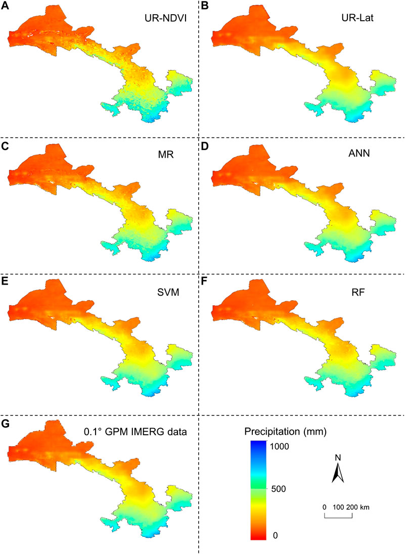
FIGURE 7. (A–F) Downscaled 1 km IMERG precipitation after residual correction in 2015 by UR-NDVI, UR-Lat, MR, ANN, SVM, and RF; (G) original 10 km GPM IMERG data in 2015.

Validation of the Downscaled Results With Rain Gauges at Annual Scale

Figures 8, 9 show the validation results of the downscaled IMERG precipitation at 1 km resolution using the rain gauge observations from 2001 to 2015 without and with residual correction, respectively. It could be seen in Figure 8 that the R² by UR-NDVI, UR-Lat, MR, ANN, SVM, and RF was 0.332, 0.677, 0.781, 0.834, 0.864, and 0.878, respectively, showing an improved performance from UR-NDVI to RF. On the contrary, the RRMSR (from 0.396 by UR-NDVI to 0.181 by RF) and RMSE (from 162.468 mm by UR-NDVI to 74.104 mm by RF) showed a degraded performance. The RF downscaling method had the best validation result, whereas the UR-NDVI method had the worst result. After the residual correction in Figure 9, the significant increase in R² and decrease in RRMSE and RMSE were found. The UR-NDVI downscaling method had the worst performance with the smallest R² and the largest RRMSE as well as RMSE. The UR-Lat, MR, and ANN methods had the approximate results after residual correction. The SVM and RF methods have better results with larger R² and smaller RRMSE as well as RMSE. In particular, we also computed the direct downscaled result by spline interpolation of the original IMERG precipitation data without any auxiliary variable (Figure 9G) and the validation result of the original IMERG precipitation (Figure 9H). The original IMERG annual precipitation data had high consistency with rain gauge data (R² = 0.884, RMSE = 74.113 mm). The direct spline spatial interpolation had better performance (R² = 0.884, RMSE = 74.095 mm) when compared with UR-NDVI, UR-Lat, MR, and ANN. However, the RRMSE and RMSE of spline interpolation were larger than those of SVM and RF.

FIGURE 8

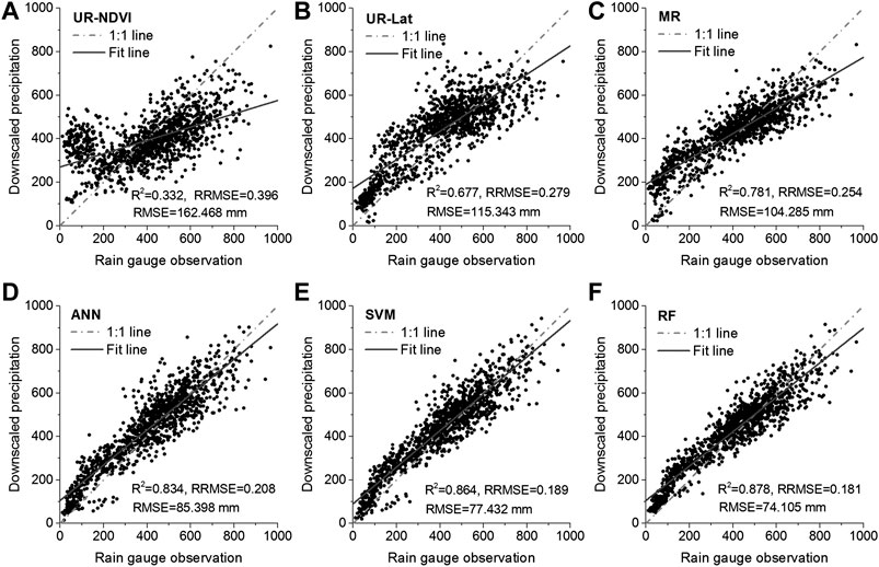
FIGURE 8. Validation results of the downscaled 1 km IMERG precipitation without residual correction using the rain gauge observations from 2001 to 2015: (A–F) UR-NDVI, UR-Lat, MR, ANN, SVM, and RF.

FIGURE 9

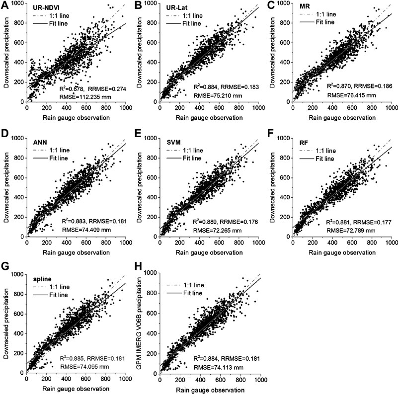
FIGURE 9. Validation results of the downscaled 1 km IMERG precipitation after residual correction using the rain gauge observations from 2001 to 2015: (A–F) UR-NDVI, UR-Lat, MR, ANN, SVM, and RF; (G) spline interpolation; (H) validation result of the original IMERG precipitation.

Table 5 shows the comparison of the mean validation results of different downscaling methods from 2001 to 2015 with and without residual correction. After residual correction, the evaluation metrics had better performances than those without residual correction. Especially, the mean RMSE in Table 5 was reduced by 44.2, 53.0, 35.7, 14.7, 7.1, and 1.8% for UR-NDVI, UR-Lat, MR, ANN, SVM, and RF, respectively, presenting an overall decreasing tendency. The parametric regression-based methods had generally great improvements, whereas the machine learning-based methods had small improvements, especially for the RF method.

TABLE 5

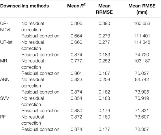
TABLE 5. Comparison of the mean evaluation metrics of the different downscaling methods from 2001 to 2015 with and without residual correction.

Performance of Different Downscaling Methods at Monthly Scale

The downscaling methods were also applied at monthly scale in accordance with the spatial downscaling procedure at annual scale. Figure 10 shows the evaluation results of different downscaling methods using the original GPM IMERG V06B data at each month from 2001 to 2015. The model performances by different downscaling methods at monthly scale were overall consistent with the results at annual scale, except for the relatively poor performance of the ANN downscaling method at monthly scale. Compared to the parametric regression downscaling methods (UR-NDVI, UR-Lat, and MR), the nonparametric regression downscaling methods (SVM and RF) had the obvious advantages, with larger R² and smaller RRMSE as well as RMSE. In terms of the monthly variability, the results of RMSE were large at the rainy seasons because of the relatively large rainfall. On the contrary, the results of RRMSE were small at the rain seasons.

FIGURE 10

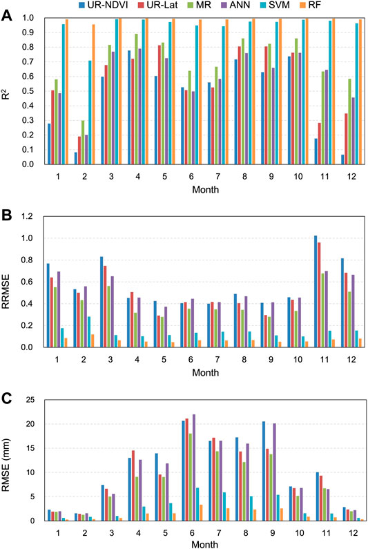
FIGURE 10. Evaluation results of different downscaling methods using the original GPM IMERG V06B data at each month from 2001 to 2015 (A-C) R2, RRMSE, and RMSE.

Table 6 shows the comparison of the evaluation metrics of different downscaling methods at monthly scale from 2001 to 2015 with and without residual correction. The SVM and RF methods had better results at monthly scale with and without residual correction. The parametric regression-based methods had great improvements after residual correction at monthly scale, whereas the machine learning based methods had small improvements. The evaluation results at monthly scale were consistent with the results at annual scale.

TABLE 6

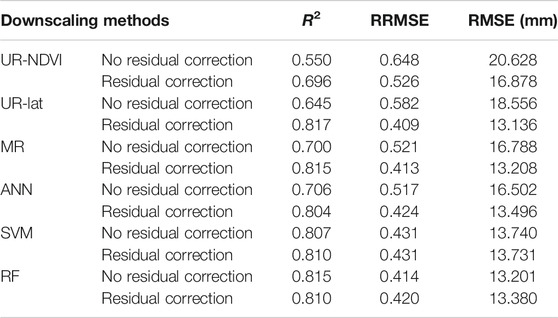
TABLE 6. Comparison of the evaluation metrics of different downscaling methods at monthly scale from 2001 to 2015 with and without residual correction.

Discussion

It has been widely acknowledged that the used auxiliary variables (land surface characteristics) in the statistic downscaling models have significant influences on the performances of the downscaled results (Jing et al., 2016; Zhang et al., 2018). NDVI is the most employed auxiliary variable in downscaling models (Duan and Bastiaanssen, 2013; Immerzeel et al., 2009; Xu et al., 2015). In this study, it was found that latitude had the largest correlation (mean R² = 0.861) with IMERG annual precipitation from 2001 to 2015 in Gansu province (Table 1). However, latitude does not vary with the year, making it limit to describe the interannual variation of precipitation distribution. Because the growth of green vegetation mainly depends on precipitation in Gansu province, the relationship between NDVI and rainfall shows high interannual variability. Therefore, both of NDVI and latitude were adopted in the UR-based downscaling models. As expected, the UR-Lat method had better performance than the UR-NDVI with larger R² and smaller RRMSE as well as RMSE both at monthly and annual scales (Table 3; Figures 3, 10). Many studies have reported that elevation has a strong effect on precipitation (Kumari et al., 2017; Tang et al., 2018); however, the relationship between elevation and precipitation was not significant in Gansu province (Table 1). The strong correlation between precipitation and elevation may be modulated in the whole study area, because the high complexity of the region is mainly distributed in the southern part of Gansu province. These results were generally consistent with the stepwise regression in the MR method and the feature importance in the RF method (Figure 4). Considering that relationship between precipitation and land surface characteristics is spatially nonstationary (Foody, 2003), five common and easily available indices (i.e., NDVI, elevation, LST, latitude, and longitude) were employed as the auxiliary variables in the MR downscaling model and three machine learning-based downscaling models. The mean R² increased and mean RRMSE as well as mean RMSE decreased from the UR methods to the MR method (Table 3), which indicated the IMERG precipitation could be better characterized by multiple auxiliary variables.

Several parametric and nonparametric regression methods have been developed to downscale the satellite precipitation in the previous studies (Chen et al., 2015; Jing et al., 2016; Retalis et al., 2017). However, this was the first study to conduct a comprehensive comparison of different algorithms for spatial downscaling of IMERG precipitation data with a relatively long time series at monthly and annual scales. It was found that the parametric regression methods had small R² and large RRMSE as well as RMSE (Figures 3, 10; Table 3), and the downscaled 1 km IMERG precipitation had obvious underestimations in the south and east of the study area and overestimations in the west (Figures 5, 6) when compared to the original 10 km IMERG precipitation. This is mainly because the UR and MR methods are global regression and the fitted functions are established in the entire region, which easily lead to overfitting and are limited to specific geographical areas where the spatial relationship between precipitation and auxiliary variables is consistent (Zhang et al., 2018). Different from parametric regression downscaling methods, the nonparametric SVM and RF downscaling methods had large R² (Figures 3, 10; Table 3) and small absolute residual errors (Figures 6D–F). It is because nonparametric regression methods have a high nonlinear adaptation and can make full use of information in the auxiliary variables (Yuan et al., 2017). As a whole, the RF downscaling method showed the best performance when compared to other downscaling methods at monthly and annual scales, demonstrating that RF algorithm could better predict the spatial heterogeneity of IMERG precipitation and was more suitable for the satellite precipitation downscaling. Similar performances of the RF algorithm for downscaling various variables (e.g., LST and leaf area index) have also been reported in other literatures (Hutengs and Vohland, 2016; Yuan et al., 2017). It is mainly because RF is a nonparametric statistical ensemble learning method, which can effectively avoid the overfitting and has better generalization ability. However, it should be noted that the predictive range of downscaled IMERG precipitation by the machine-learning based methods is restricted to the range covered by the training data (Hutengs and Vohland, 2016). Therefore, all pixels over the entire region (Gansu province) at 10 km resolution were used as the training data in this study to avoid this limitation.

The performance of residual correction has been preliminarily discussed in the previous studies (Jing et al., 2016; Xu et al., 2015). The purpose of residual correction is to reduce the residual errors (the part of the precipitation cannot be explained by the auxiliary factors) in the downscaling procedure. In this study, we found that the downscaled IMERG precipitation after residual correction had more similar spatial patterns to the original 10 km GPM IMERG V06B precipitation data (Figure 7), compared to the downscaled IMERG precipitation without residual correction (Figure 6). Especially for the parametric regression methods (UR-NDVI, UR-Lat, and MR), the validation results of downscaled precipitation with and without residual correction had significant differences (Figures 8, 9). Xu et al. (2015) have pointed out that the residual error is an important error source of the downscaled results in the MR downscaling method, which can be alleviated after residual correction. However, it has been reported by Jing et al. (2016) that the accuracy of the downscaled results has no improvement after residual correction. The residual errors represent the precipitation variation, which cannot be explained by the auxiliary variables. In this study, the reduced percentage of RMSE after residual correction decreased from UR-NDVI to RF (Tables 5, 6). The parametric regression methods had large improvements, while the improvements were very small for the machine-learning based methods, especially for RF. It was mainly because the spatial variation of IMERG precipitation at monthly and annual scales had been well predicted by the machine learning-based downscaling models before residual correction. It should be noted that, at present, the residual error at 1 km resolution is generally obtained using the sample spline interpolation method (Immerzeel et al., 2009; Jia et al., 2013). This interpolation algorithm included in residual correction also faces the challenge of precipitation spatial heterogeneity (Chen et al., 2015) and can cause certain errors in the downscaled results. Therefore, we recommend using the downscaling method with better predictive ability of precipitation spatial heterogeneity (e.g., SVM and RF) to avoid residual correction.

Although rarely discussed, it must be pointed out that the accuracy of the original satellite precipitation data has a great influence on the downscaling results, regardless of the downscaling methods and the auxiliary variables. A large number of studies have shown that the GPM-era precipitation products have better accuracy as well as higher resolution than those in the TRMM-era (Tang et al., 2016; Chen et al., 2018; Peng et al., 2020). A comparative study has shown that the downscaled results based on IMERG V05B precipitation had better performance than those based on TMPA precipitation over the Tibetan Plateau in 2015 (Ma et al., 2018). Therefore, the spatial downscaling of the latest released IMERG precipitation with a relatively long time series may practically provide more accurate precipitation data for the hydrological application at catchment scales. In addition, the downscaling procedure is based on the assumption that the empirical statistical relationship established at low/coarse spatial resolution is also applicable at high/fine spatial resolution. Our previous study has shown that the precipitation-NDVI relationships are approximate at different scales (0.25°–1.0°) in Gansu province (Chen et al., 2015). Therefore, it was assumed that the statistical relationship is scale independent in this study. However, Immerzeel et al. (2009) found that the optimal fitting resolution of precipitation-NDVI relationships at multiple scales (0.25°–1.25°) was 0.75°. The scale-independent issue should be paid special attention in future studies. Since the main purpose of this study was to compare the performance of different downscaling methods, we just selected five commonly used auxiliary variables. However, it should be noted that the auxiliary variables usually have different performances in different regions or even in the same region but with different temporal scales (Jing et al., 2016; Ma et al., 2020). Therefore, a comparison study of the performance of different downscaling methods in different regions and on different temporal scales (e.g., weekly and daily scales) could be interesting topics in future studies.

Conclusion

A comprehensive comparison study of different methods for spatial downscaling of GPM IMERG V06B monthly and annual precipitation with a relatively long time series from 2001 to 2015 was conducted by selecting five commonly used auxiliary variables. Latitude had the largest correlation with IMERG annual precipitation in Gansu province, but it is limited to describe the interannual variation of precipitation distribution. The most employed NDVI had the second largest R² with IMERG annual precipitation. The performances of different downscaling methods showed a similarity from 2001 to 2015. On the whole, the performances of the different downscaling methods at annual scale were in the order UR-NDVI (worst) < UR-Lat < MR < ANN < SVM < RF (best). The downscaled results at monthly scale were overall consistent with the results at annual scale. The downscaled 1 km IMERG precipitation by parametric regression methods had obviously deviations, whereas the machine learning-based methods could capture the spatial heterogeneity of precipitation, with larger R² and smaller RMSE as well as RRMSE. The deviations caused by the parametric regression methods could be compensated after residual correction; however, the residual correction is not recommended since the involved spline interpolation procedure may cause certain errors in the downscaled results. The machine learning-based RF downscaling method had the most robust performance with smallest residual errors and the overall best validation results, which could be an effective way to provide accurate precipitation with sufficient spatial details for hydrological application at the catchment scales.

Data Availability Statement

The datasets generated for this study are available on request to the corresponding author.

Author Contributions

CC conceptualized the study, was involved in the methodology, and wrote and prepared the original draft; QC was responsible for writing, reviewing, and editing; BQ curated the data; SZ supervised the study; ZD was involved in the conceptualization, writing, reviewing, and editing.

Funding

This work was supported by the by the National Key Research and Development Program of China (2017YFC0404501), National Natural Science Foundation of China (51709179), and Natural Science Foundation of Jiangsu Province (BK20181262). ZD is grateful for the financial support for this research from the Royal Physiographic Society in Lund (2019-40630), and Faculty of Science at Lund University, Sweden.

Conflict of Interest

The authors declare that the research was conducted in the absence of any commercial or financial relationships that could be construed as a potential conflict of interest.

References

Ashouri, H., Hsu, K.-L., Sorooshian, S., Braithwaite, D. K., Knapp, K. R., Cecil, L. D., et al. (2015). PERSIANN-CDR: Daily precipitation climate data record from multisatellite observations for hydrological and climate studies. Bull. Am. Meteorol. Soc. 96 (1), 69–83. doi:10.1175/bams-d-13-00068.1.

CrossRef Full Text | Google Scholar

Breiman, L. (2001). Random forests. Mach. Learn. 45 (1), 5–32. doi:10.1023/a:1010933404324.

CrossRef Full Text | Google Scholar

Chang, C.-C., and Lin, C.-J. (2011). Library for support vector machines. ACM Trans. Intell. Syst. Technol. 2 (3), 1–27. doi:10.1145/1961189.1961199.

CrossRef Full Text | Google Scholar

Chen, C., Chen, Q., Duan, Z., Zhang, J., Mo, K., Li, Z., et al. (2018). Multiscale comparative evaluation of the GPM IMERG v5 and TRMM 3B42 v7 precipitation products from 2015 to 2017 over a climate transition area of China. Rem. Sens. 10 (6), 944. doi:10.3390/rs10060944.

CrossRef Full Text | Google Scholar

Chen, C., Li, Z., Song, Y., Duan, Z., Mo, K., Wang, Z., et al. (2020). Performance of multiple satellite precipitation estimates over a typical arid mountainous area of China: spatiotemporal patterns and extremes. J. Hydrometeorol. 21 (3), 533–550. doi:10.1175/jhm-d-19-0167.1.

CrossRef Full Text | Google Scholar

Chen, C., Zhao, S., Duan, Z., and Qin, Z. (2015). An improved spatial downscaling procedure for TRMM 3B43 precipitation product using geographically weighted regression. IEEE J. Sel. Top. Appl. Earth Obs. Remote Sens. 8 (9), 4592–4604. doi:10.1109/jstars.2015.2441734.

CrossRef Full Text | Google Scholar

Duan, Z., and Bastiaanssen, W. G. M. (2013). First results from Version 7 TRMM 3B43 precipitation product in combination with a new downscaling-calibration procedure. Remote Sens. Environ. 131, 1–13. doi:10.1016/j.rse.2012.12.002.

CrossRef Full Text | Google Scholar

Fang, J., Du, J., Xu, W., Shi, P., Li, M., and Ming, X. (2013). Spatial downscaling of TRMM precipitation data based on the orographical effect and meteorological conditions in a mountainous area. Adv. Water Resour. 61, 42–50. doi:10.1016/j.advwatres.2013.08.011.

CrossRef Full Text | Google Scholar

Foody, G. M. (2003). Geographical weighting as a further refinement to regression modelling: An example focused on the NDVI-rainfall relationship. Remote Sens. Environ., 88 (3), 283–293. doi:10.1016/j.rse.2003.08.004.

CrossRef Full Text | Google Scholar

Hou, A. Y., Kakar, R. K., Neeck, S., Azarbarzin, A. A., Kummerow, C. D., Kojima, M., et al. (2014). The global precipitation measurement mission. Bull. Am. Meteorol. Soc. 95 (5), 701–722. doi:10.1175/bams-d-13-00164.1.

CrossRef Full Text | Google Scholar

Huffman, G. J., Bolvin, D. T., Nelkin, E. J., Wolff, D. B., Adler, R. F., Gu, G., et al. 2007). The TRMM multisatellite precipitation analysis (TMPA): Quasi-global, multiyear, combined-sensor precipitation estimates at fine scales. J. Hydrometeorol. 8 (1), 38–55. doi:10.1175/jhm560.1.

CrossRef Full Text | Google Scholar

Hutengs, C., and Vohland, M. (2016). Downscaling land surface temperatures at regional scales with random forest regression. Remote Sens. Environ. 178, 127–141. doi:10.1016/j.rse.2016.03.006.

CrossRef Full Text | Google Scholar

Immerzeel, W. W., Rutten, M. M., and Droogers, P. (2009). Spatial downscaling of TRMM precipitation using vegetative response on the Iberian Peninsula. Remote Sens. Environ. 113 (2), 362–370. doi:10.1016/j.rse.2008.10.004.

CrossRef Full Text | Google Scholar

Jia, S., Zhu, W., Lű, A., and Yan, T. (2011). A statistical spatial downscaling algorithm of TRMM precipitation based on NDVI and DEM in the Qaidam Basin of China. Remote Sens. Environ. 115 (12), 3069–3079. doi:10.1016/j.rse.2011.06.009.

CrossRef Full Text | Google Scholar

Jing, W., Yang, Y., Yue, X., and Zhao, X. (2016). A spatial downscaling algorithm for satellite-based precipitation over the Tibetan plateau based on NDVI, DEM, and land surface temperature. Remote Sens. 8 (8), 655. doi:10.3390/rs8080655.

CrossRef Full Text | Google Scholar

Kidd, C., and Levizzani, V. (2011). Status of satellite precipitation retrievals. Hydrol. Earth Syst. Sci. 15 (4), 1109–1116. doi:10.5194/hess-15-1109-2011.

CrossRef Full Text | Google Scholar

Kubota, T., Shige, S., Hashizume, H., Aonashi, K., Takahashi, N., Seto, S., et al. (2007). Global precipitation map using satellite-borne microwave radiometers by the GSMaP project: production and validation. IEEE Trans. Geosci. Remote Sens. 45 (7), 2259–2275. doi:10.1109/tgrs.2007.895337.

CrossRef Full Text | Google Scholar

Kumari, M., Singh, C. K., Bakimchandra, O., and Basistha, A. (2017). Geographically weighted regression based quantification of rainfall-topography relationship and rainfall gradient in Central Himalayas. Int. J. Climatol. 37 (3), 1299–1309. doi:10.1002/joc.4777.

CrossRef Full Text | Google Scholar

López, L. P., Immerzeel, W. W., Rodríguez Sandoval, E. A., Sterk, G., and Schellekens, J. (2018). Spatial downscaling of satellite-based precipitation and its impact on discharge simulations in the Magdalena River basin in Colombia. Front. Earth Sci. 6, 68. doi:10.3389/feart.2018.00068

CrossRef Full Text | Google Scholar

Liaw, A., and Wiener, M. (2002). Classification and regression by randomForest. R News. 2 (3), 18–22.

Google Scholar

Liu, Q., McVicar, T. R., Yang, Z., Donohue, R. J., Liang, L., and Yang, Y. (2016). The hydrological effects of varying vegetation characteristics in a temperate water-limited basin: development of the dynamic Budyko-Choudhury-Porporato (dBCP) model. J. Hydrol. 543, 595–611. doi:10.1016/j.jhydrol.2016.10.035.

CrossRef Full Text | Google Scholar

Lu, X., Wei, M., Tang, G., and Zhang, Y. (2018). Evaluation and correction of the TRMM 3B43V7 and GPM 3IMERGM satellite precipitation products by use of ground-based data over Xinjiang, China. Environ. Earth Sci. 77 (5), 209. doi:10.1007/s12665-018-7378-6.

CrossRef Full Text | Google Scholar

Ma, Y., Tang, G., Long, D., Yong, B., Zhong, L., Wan, W., et al. (2016). Similarity and error intercomparison of the GPM and its predecessor-TRMM multisatellite precipitation analysis using the best available hourly gauge network over the Tibetan Plateau. Remote. Sens. 8 (7), 569. doi:10.3390/rs8070569.

CrossRef Full Text | Google Scholar

Ma, Z., He, K., Tan, X., Xu, J., Fang, W., He, Y., et al. (2018). Comparisons of spatially downscaling TMPA and IMERG over the Tibetan Plateau. Remote. Sens. 10 (12), 1883. doi:10.3390/rs10121883.

CrossRef Full Text | Google Scholar

Ma, Z., Xu, J., He, K., Han, X., Ji, Q., Wang, T., et al. (2020). An updated moving window algorithm for hourly-scale satellite precipitation downscaling: a case study in the Southeast Coast of China. J. Hydrol. 581, 124378. doi:10.1016/j.jhydrol.2019.124378.

CrossRef Full Text | Google Scholar

Maisongrande, P., Duchemin, B., and Dedieu, G. (2004). VEGETATION/SPOT: an operational mission for the earth monitoring; presentation of new standard products. Int. J. Remote Sens. 25 (1), 9–14. doi:10.1080/0143116031000115265.

CrossRef Full Text | Google Scholar

Nourani, V., Baghanam, A. H., and Gokcekus, H. (2018). Data-driven ensemble model to statistically downscale rainfall using nonlinear predictor screening approach. J. Hydrol. 565, 538–551. doi:10.1016/j.jhydrol.2018.08.049.

CrossRef Full Text | Google Scholar

Peng, F., Zhao, S., Chen, C., Cong, D., Wang, Y., and Ouyang, H. (2020). Evaluation and comparison of the precipitation detection ability of multiple satellite products in a typical agriculture area of China. Atmos. Res. 236, 104814. doi:10.1016/j.atmosres.2019.104814.

CrossRef Full Text | Google Scholar

Retalis, A., Tymvios, F., Katsanos, D., and Michaelides, S. (2017). Downscaling CHIRPS precipitation data: an artificial neural network modelling approach. Int. J. Remote Sens. 38 (13), 3943–3959. doi:10.1080/01431161.2017.1312031.

CrossRef Full Text | Google Scholar

Rodríguez, E., Morris, C. S., and Belz, J. E. (2006). A global assessment of the SRTM performance. Photogramm. Eng. Remote Sensing. 72 (3), 249–260. doi:10.14358/pers.72.3.249.

CrossRef Full Text | Google Scholar

Sachindra, D. A., and Perera, B. J. C. (2016). Statistical downscaling of general circulation model outputs to precipitation accounting for non-stationarities in predictor-predictand relationships. PloS One. 11 (12). doi:10.1371/journal.pone.0168701. | Pubmed

CrossRef Full Text | Google Scholar

Sharifi, E., Saghafian, B., and Steinacker, R. (2019). Downscaling satellite precipitation estimates with multiple linear regression, artificial neural networks, and spline interpolation techniques. J. Geophys. Res. Atmos. 124 (2), 789–805. doi:10.1029/2018jd028795.

CrossRef Full Text | Google Scholar

Shen, Y., Xiong, A., Wang, Y., and Xie, P. (2010). Performance of high‐resolution satellite precipitation products over China. J. Geophys. Res.: Atmosphere. 115 (D2). doi:10.1029/2009jd012097.

CrossRef Full Text | Google Scholar

Shi, Y., Song, L., Xia, Z., Lin, Y., Myneni, R., Choi, S., et al. (2015). Mapping annual precipitation across mainland China in the period 2001-2010 from TRMM3B43 product using spatial downscaling approach. Remote Sens. 7 (5), 5849–5878. doi:10.3390/rs70505849.

CrossRef Full Text | Google Scholar

Song, X., Duan, Z., and Jiang, X. (2012). Comparison of artificial neural networks and support vector machine classifiers for land cover classification in Northern China using a SPOT-5 HRG image. Int. J. Remote Sens. 33 (10), 3301–3320. doi:10.1080/01431161.2011.568531.

CrossRef Full Text | Google Scholar

Tang, G., Long, D., Hong, Y., Gao, J., and Wan, W. (2018). Documentation of multifactorial relationships between precipitation and topography of the Tibetan Plateau using spaceborne precipitation radars. Remote Sens. Environ. 208, 82–96. doi:10.1016/j.rse.2018.02.007.

CrossRef Full Text | Google Scholar

Tang, G., Ma, Y., Long, D., Zhong, L., and Hong, Y. (2016). Evaluation of GPM Day-1 IMERG and TMPA Version-7 legacy products over Mainland China at multiple spatiotemporal scales. J. Hydrol. 533, 152–167. doi:10.1016/j.jhydrol.2015.12.008.

CrossRef Full Text | Google Scholar

Vapnik, V. (1995). The nature of statistical learning theory. New York, NY:Springer

Google Scholar

Wan, Z. (2008). New refinements and validation of the MODIS land-surface temperature/emissivity products. Remote Sens. Environ., 112(1), 59–74. doi:10.1016/j.rse.2006.06.026.

CrossRef Full Text | Google Scholar

Wilby, R. L., and Wigley, T. M. L. (2000). Precipitation predictors for downscaling: observed and general circulation model relationships. Int. J. Climatol. 20 (6), 641–661. doi:10.1002/(sici)1097-0088(200005)20:6<641::aid-joc501>3.0.co;2-1.

CrossRef Full Text | Google Scholar

Xu, S., Wu, C., Wang, L., Gonsamo, A., Shen, Y., and Niu, Z. (2015). A new satellite-based monthly precipitation downscaling algorithm with non-stationary relationship between precipitation and land surface characteristics. Remote Sens. Environ. 162, 119–140. doi:10.1016/j.rse.2015.02.024.

CrossRef Full Text | Google Scholar

Yuan, H., Yang, G., Li, C., Wang, Y., Liu, J., Yu, H., et al. (2017). Retrieving soybean leaf area index from unmanned aerial vehicle hyperspectral remote sensing: analysis of RF, ANN, and SVM regression models. Remote Sens., 9 (4), 309. doi:10.3390/rs9040309.

CrossRef Full Text | Google Scholar

Zhang, T., Li, B., Yuan, Y., Gao, X., Sun, Q., Xu, L., et al. (2018). Spatial downscaling of TRMM precipitation data considering the impacts of macro-geographical factors and local elevation in the three-river headwaters region. Remote Sens. Environ. 215, 109–127. doi:10.1016/j.rse.2018.06.004.

CrossRef Full Text | Google Scholar

Zhao, N., Yue, T., Zhou, X., Zhao, M., Liu, Y., Du, Z., et al. (2017). Statistical downscaling of precipitation using local regression and high accuracy surface modeling method. Theor. Appl. Climatol., 129 (1–2), 281–292. doi:10.1007/s00704-016-1776-z.

CrossRef Full Text | Google Scholar