Pore Network Modeling of Core Forming Melts in Planetesimals

Early in the history of the solar system, planetesimals were differentiated into metallic cores. In some planetesimals, this differentiation took place by percolation of the denser core forming liquid through a lighter solid silicate matrix. A key factor in core formation by percolation is the establishment of a connection threshold of the melt. In this work, we report new results from pore network modeling of 3D microtomographic images of 11 synthetic olivine aggregates containing Fe-FeS melt. Our results demonstrate that a melt volume fraction of 0.14 is required to achieve connectivity of the melt. We also show that surface-tension driven melt segregation during annealing experiments plays an important role in controlling this threshold melt fraction. We also report that, contrary to the generally accepted notion, melt pinch-off is caused by reduction in pore size, rather than melt drainage out of throats. Using the results of our study, we estimate that the peak melt segregation velocity in a planetesimal of 100 km radius can be as high as 41 m/yr and core segregation can be completed in less than 0.5 million years.

1. Introduction

Planetesimals—parent bodies of meteorites and building blocks of terrestrial planets—were differentiated into metallic cores overlain by a silicate mantle and crust early in the history of the solar system (Rubie, 2007; Weiss and Elkins-Tanton, 2013). Based on the temperature within the planetesimal, such diffrentiation plausibly took place by two different mechanisms (Rubie, 2007; Rushmer and Watson, 2015). The first mechanism involved large scale melting—the magma ocean stage—of the planetesimal. The heat required to produce such large scale melting could be provided by decay of short-lived radioactive isotopes such as ²⁶Al and ⁶⁰Fe, energy released due to impact with other planetesimals, or release of gravitational energy arising from the process of core segregation (Stevenson, 1990; Tonks and Melosh, 1990; Rubie, 2007; Elkins-Tanton, 2012). The timing of core segregation under such conditions depends on the length of time the magma ocean remains molten (Abe, 1997; Elkins-Tanton, 2012; Hier-Majumder and Hirschmann, 2017) and the time taken by metallic droplets, suspended by turbulent convection in the magma ocean (Solomatov and Stevenson, 1993; Solomatov, 2000), to sink to the bottom.

The second mechanism of core formation, percolation of Fe-FeS melts through a solid silicate matrix, operated when the internal temperature of the planetesimal was above the melting point of metallic melts in the Fe-FeS composition space, but below the melting point of the silicates (Stevenson, 1990; Rubie, 2007). At the surface of the planetesimal, where core formation by percolation initiated, the difference between these two melting points were substantial. For example, the surface melting temperature on the martian mantle solidus is 1088^oC (Duncan et al., 2018) while it is 1120^oC on the terrestrial solidus (Hirschmann, 2000). In contrast, the eutectic melting temperature of FeS melts—at which the first melting takes place, independent of relative abundances of Fe and S in the bulk composition—is 988^oC at atmospheric pressure (Ryzhenko and Kennedy, 1973). Cosmochemical evidence based on Hf-W and Fe isotopes indicate that such processes were operative within the interiors of parent bodies of some meteorties (Kruijer et al., 2014; Barrat et al., 2015; Budde et al., 2015). The rate of melt percolation through the solid matrix depended on the establishment of a connected melt network and the velocity with which the melt segregated to form the core. Cosmochemical models estimate that percolative core formation in the mostly solid planetesimals possibly took place between 0.5 and 1 Ma (Kruijer et al., 2014). To explain this cosmochemical constraint and understand the early stages of evolution of terrestrial planets, it is important to constrain the “connection threshold,” the melt volume fraction at which a connected network of core forming melts was established (Minarik, 2003).

The connectivity of core forming melts in an olivine matrix has been studied in a number of previous works (Yoshino et al., 2003; Roberts et al., 2007; Bagdassarov et al., 2009a,b; Watson and Roberts, 2011; Ghanbarzadeh et al., 2017), with somewhat diverging results. Some of these studies detect the threshold of connectivity of Fe-FeS melts in olivine by a drastic increase in electrical conductivity (Yoshino et al., 2003; Roberts et al., 2007; Bagdassarov et al., 2009a; Watson and Roberts, 2011). Roberts et al. (2007) and Watson and Roberts (2011) also studied 3D microtomographic images of small subvolumes within their samples in addition to electrical conductivity measurements. In the group of experiments where the samples were annealed for 24 h or less, the connection threshold was observed around total melt fraction of 5–6 vol% (Yoshino et al., 2003; Roberts et al., 2007; Watson and Roberts, 2011). In contrast, laboratory experiments where the samples were annealed for 72 h (Bagdassarov et al., 2009a,b), the connection threshold was much higher, near 16 vol%, in agreement with numerical models of Fe-FeS melt in a matrix containing irregular shaped grains (Ghanbarzadeh et al., 2017, 10–19 vol%). To address the discrepancy between these two sets of observations, we present the first results of direct pore network modeling of melt connectivity from microtomographic images of samples annealed by Solferino et al. (2015) and Solferino and Golabek (2018). In these experiments, samples consisting of Fe-FeS melt in an olivine matrix were annealed between 40 and 360 h. To constrain the conditions for the establishment of the connected network of core forming minerals, it is important to consider the textural evolution of partially molten aggregates.

The process of textural maturation in partially molten aggregates, liquid phase sintering (German, 2013), involves simultaneous grain growth and melt redistribution, primarily driven by surface tension. The aspect of grain growth in the samples used in our study were reported in detail by Solferino et al. (2015) and Solferino and Golabek (2018). In this work, we focus on the second aspect of textural maturation involving melt redistribution driven by surface tension (Hier-Majumder et al., 2006; Takei and Hier-Majumder, 2009; King et al., 2011). In so-called “wetting” systems, marked by solid-melt dihedral angles less than 60^o (Wray, 1976), the tension along grain-grain interfaces is stronger than that along grain-melt interface. As a result, surface tension tends to homogenize uneven distribution of local large concentrations of melt (King et al., 2011). The opposite behavior is expected in “non-wetting” systems where the tension on grain-melt interfaces is higher than that on the grain-grain interfaces. Theoretical models predict that with time, the melt is expected to self segregate into local regions of relatively high concentrations of melt (Hier-Majumder et al., 2006). This theoretical prediction of self separation of non-wetting, core forming melts are yet to be tested by microtomographic image analysis.

In this article, we address the influence of connection threshold of Fe-FeS melts on the timing of core formation of planetesimals. The first goal of this article is to directly measure the connectivity of the Fe-FeS melt network from the microtomographic images of samples annealed for times exceeding 24 h. Our second goal is to compare the results from the two different sets of experiments and explain the possible discrepancies. The final goal of this article is to provide an estimate for the segregation velocity of core forming melts and constrain the time of core segregation by percolation in planetesimals.

2. Methods

In this section, we present a brief description of the experimental samples used for microtomographic measurements and the method of image analysis and pore network modeling.

2.1. Synthetic Olivine-Fe-FeS Aggregates

The synthetic olivine-Fe-FeS aggregates used in this study were annealed in an end-loaded piston cylinder press at a pressure of 1 GPa (Solferino et al., 2015; Solferino and Golabek, 2018). Details of the starting materials and the experimental methodology are reported in the aforementioned articles. A summary of experimental conditions, compositions, and results from 2D grain size measurements are reported in Table 1. The samples in these two studies consisted of the same olivine powder mixed with two different proportions of Fe and S. The olivine powder used to synthesize the samples imaged in this study was milled down to an average size of 1.8 μm and fragment size distribution was measured with laser diffractometry, proving a single peak in the size distribution curve (Solferino et al., 2015; Solferino and Golabek, 2018). The starting average fragment size and the shape of the fragment distribution curve influence the time elapsed to reach textural equilibrium (Faul and Scott, 2006).

TABLE 1

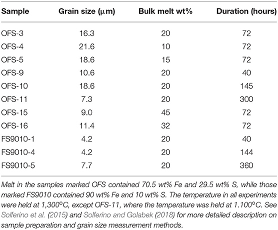
Table 1. Summary of experimental conditions and grain size of the synthetic samples.

In this study, we imaged 8 samples containing a mixture of olivine and a melt comprising of 70.5 wt% Fe and 29.5 wt% S (samples labeled OFS by Solferino and Golabek, 2018). We also imaged another 3 samples containing 90 wt% Fe and 10 wt% S (samples labeled FS by Solferino and Golabek, 2018). Detailed composition of these samples, obtained by electron microprobe analysis, are provided in Table 2 of both articles (Solferino et al., 2015; Solferino and Golabek, 2018). The temperature in all but one of these experiments was 1,300^oC, with the exception of the experiment OFS-11 where the temperature was 1,100^oC. The annealing time for these experiments ranged between 40 and 360 h. The average grain size in the two Fe-rich samples were around 4 μm (Solferino and Golabek, 2018) while the grain size in the samples with eutectic mixtures varied between 7 μm and 19 μm.

TABLE 2

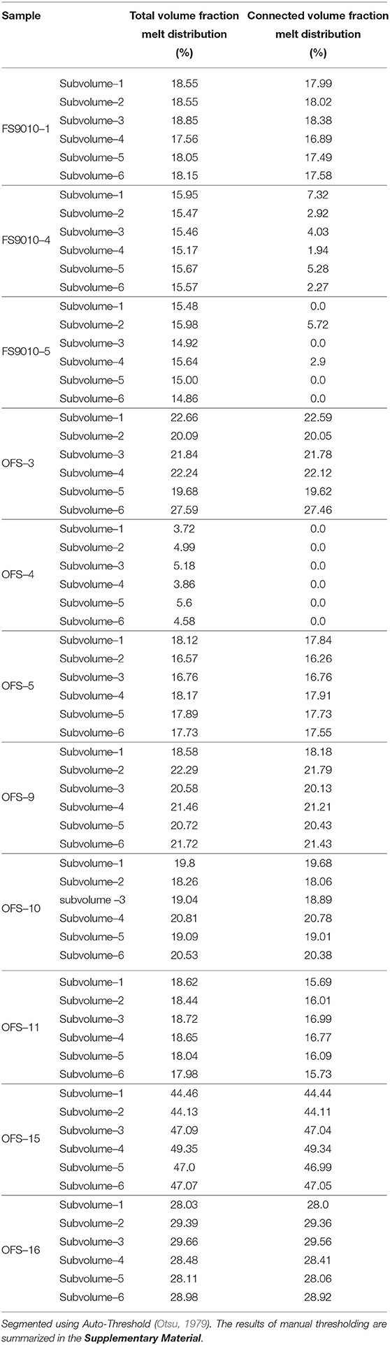
Table 2. Results of melt distribution volume calculation.

2.2. Image Acquisition and Filtering

We constructed 3D volumes from a stack of 2D microtomographic images, acquired at the the beamline “Tomographic Microscopy and Coherent Radiology Experiments” (TOMCAT)—dedicated to microtomographic studies—at the Swiss Light Source at Paul Scherrer Institut, Switzerland. Images of longitudinal sections of whole sample capsules, consisting of a graphite half-cylinder enclosing the annealed olivine and Fe-S, were acquired with a pixel resolution of 0.325 μm, at beam energies between 29 and 33 keV. Each stack of images were acquired at a constant beam energy. A Lutetium Aluminum Garnet (LuAg:Ce) scintillator crystal was used, with a detector magnification of 20X and an exposure time of 1400 ms. The raw images were further processed to extract propagation-induced phase contrast images (Paganin et al., 2002). The 2D images were stacked in a grid—equidistant from each other, with the spacing between slices calculated from the height of the stack and the number of images—using the commercial software PerGeos to create a 3D volume. Each stack of 2D grayscale images was then filtered and segmented using PerGeos to extract the matrix and melt phases.

The first step in image analysis involved filtering the stack of 2D grayscale images acquired during microtomography. During this step, we removed image artifacts created during image acquisition (Ketcham and Carlson, 2001; Wildenschild et al., 2002). Image filtering also reduced spurious noise without removing significant details, enhanced the contrast between the key phases, and improved overall image quality. In this work, we used the non-local means filter (Buades et al., 2005) to boost the signal-to-noise ratio in the 2D X-ray images. The algorithm behind this filter deploys a large search window from which a weighted average of grayscale values is used to determine the grayscale of the current voxel under consideration (Buades et al., 2005, 2008; Schluter et al., 2014). This highly efficient noise removal filter exerts quality smoothing in homogeneous regions. Figure 1 demonstrates an example of a 2D slice from the sample OFS-5 before (a) and after (b) filtering using the non-local means algorithm. The zoomed insets show the pixelated texture before (a) and smoothed texture after (b).

FIGURE 1

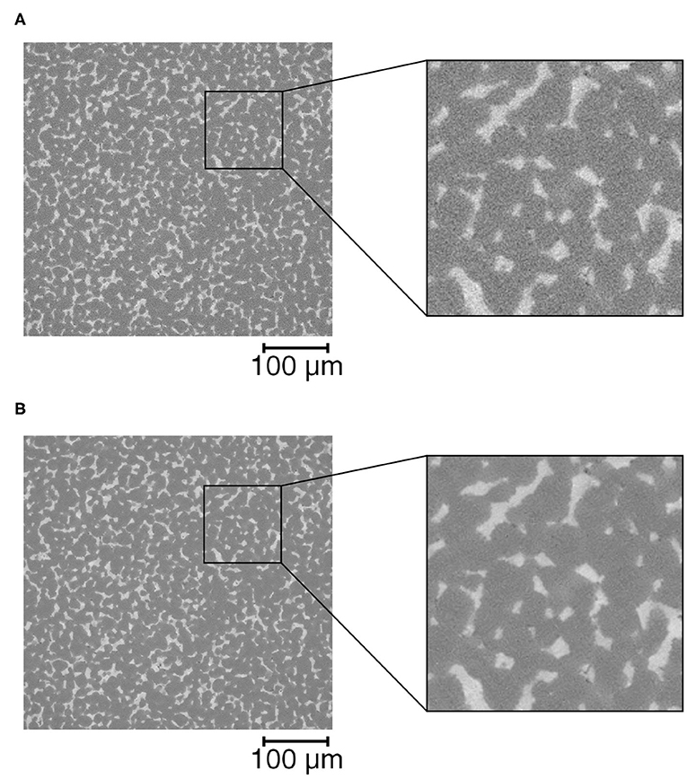
Figure 1. Before and after filtering of images using non-local means algorithm. Panel (A) shows a raw 2D slice through the whole sample OFS-5, with inset showing the pixelated texture present in raw data. Panel (B) shows the same 2D slice following the image filtering. The inset shows the improved quality of the image with effective smoothing of different phases.

2.3. Segmentation and Volume Fraction Determination

To quantify the melt volume fractions in the samples, we segmented entire volumes of the filtered 3D images, assigning distinct labels to the Fe-FeS melt and the olivine matrix. Distinct grayscale values, arsing from the composition of each phase, were used to label each voxel in the 3D volume. We used both manual and automated segmentation methods to separate the phases and calculate melt volume fraction and connectivity.

In the manual segmentation method, we inspected the grayscale intensity histogram of each 3D volume, determining the threshold based on a broad peak nearer the higher intensity end of the scale. Figure 2A shows a 2D filtered slice of sample OFS-10. The melt distribution is shown in lighter shades of gray. The results of manual thresholding of the same slice are displayed in Figure 2B. We provide the threshold range used for manual segmentation of the 3D volumes in the data table in section 2 of the Supplementary Material. In addition, we used an automated method to select the threshold grayscale intensity and compare measures. The auto-threshold method uses Otsu's algorithm (Otsu, 1979). In this technique, the threshold is selected by minimizing the weighted within-class variance. Assigning the Otsu algorithm to target the high intensity voxels representative of the melt distribution, we performed the separation on each of the subvolumes in all samples. The algorithm is most effective for images that display a bimodal distribution in the image histogram.

FIGURE 2

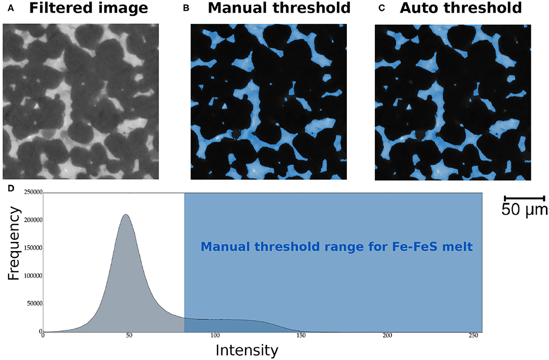
Figure 2. Comparison between manual and auto threshold techniques using a 2D slice from sample OFS-10 – subvolume 1. Panel (A) shows the image filtering result using the non-local means technique. The segmentation of the melt distribution using the manual threshold is shown in (B), while the results of auto threshold are shown in (C). (D) A representative histogram from a 2D slice of sample OFS-10. The pronounced peak near the intensity of 50 represents gray scale values of olivine grains. The shaded blue region marks the intensity range defined as the melt phase during manual thresholding. Manual threshold ranges for each subvolumes are provided in the Supplementary Material. See text and references therein for more information on the automated thresholding.

A number of previous studies discussed the merits and drawbacks of both methods of segmentation (Pal and Pal, 1993; Trier and Jain, 1995; Sezgin and Sankur, 2004; Iassonov et al., 2009). While the automated thresholding method overcomes the issue of operator bias, the pore volume fraction can be over or underestimated by this method (Thomson et al., 2018, 2019). In the online supplemental data (Hier-Majumder et al., 2020), we report the melt volume fraction determined by both methods. Given the strong contrast in the gray scale intensity values of olivine and Fe-FeS melts, we prefer the volume fractions obtained by automated segmentation, which are used in the figures and reported in Table 2 in the main article. To calculate the uncertainty in the measured total and connected melt volume fractions, we use the difference between the volume fractions obtained by these two methods. Figures 2B,C highlight the segmentation results of manual and auto-threshold methods on the same 2D slice. Figure 2D highlights the representative histogram from a 2D slice of sample OFS-10. The peak near the intensity of 50 corresponds to gray scale values of olivine grains in the sample, while the shaded blue region is the intensity range assigned to the melt phase during manual threshold segmentation. Once the 3D volumes were segmented into the melt and matrix phases, we selected representative subvolumes to carry out further analyses.

We created 6 subvolumes (SV) of dimension 200 μm³ (615 × 615 × 615 voxels) within each of the 11 samples imaged by microtomography, leading to a total of 66 subvolumes. Figure 3A shows the total volume for sample OFS-3 and an example of one subvolume (SV2). Small subvolumes are selected to target regions of homogeneous melt distribution and avoid small scale heterogeneity in the samples. Figure 3B is an example of a 2D slice taken from SV2 in sample OFS-3. The 3D volume rendering of this subvolume indicates that this region remains largely homogeneous, with the exception of some larger pockets of melt found at the edges (Figure 3C). We present a more detailed discussion about the differences between our subvolumes and those of Watson and Roberts (2011) in section 4.1.

FIGURE 3

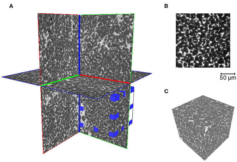
Figure 3. Sub-sample selection figure. The whole volume for sample OFS-3 – is shown in (A), with subvolume 2 highlighted by the small cube with blue marked edges. A 2D slice through the subvolume is displayed in (B), and a 3D volume rendered image of the whole subvolume is shown in (C).

To evaluate the connectivity of different melt distributions, the binary images (produced as a result of the segmentation process described above) require further processing. The total melt volume fraction is then calculated by dividing the number of voxels in the melt phase by the total number of voxels in the subvolume. To measure the connected melt fraction, the total melt volume is processed using an axis-connectivity algorithm. This algorithm assumes a plane at the top and bottom of one axis and calculates all voxels that form a connected network in between. Voxels that do not form part of the connected network are removed by the algorithm and a new binary image, containing only the connected melt voxels, is generated. The number of these connected voxels are then divided by the total number of voxels in the subvolume to calculate the connected melt fraction.

2.4. Pore Network Modeling

While the segmentation and axis-connectivity algorithm provide information about volume fractions, they are unable to characterize individual melt-filled pores. To quantify the dimension and degree of connectivity of individual melt-filled pores, we build pore network models (PNMs) within each subvolume for both the total and connected melt fractions in the subvolume. The PNM decomposes the melt network into pores, melt pockets located at grain corners, and throats, channel that connect two pores. For each pore, the PNM also generates a coordination number, the number of throats connected to the pore. Pores belonging to a connected network must at least possess a coordination number of 2. This pore network construction can be considered equivalent to a train transport network. In this analogy, junction stations, where more than one tracks meet, are equivalent to pores, and the train tracks are equivalent to throats. Interested readers can consult the textbook by Blunt (2017, Ch. 2)for more detailed discussion on the elements of the PNM.

To construct a PNM, the geometry and topology of the melt distribution is required. The binary images (acquired from image segmentation) of the melt volume are processed directly by a hybrid algorithm (Youssef et al., 2007). The algorithm creates a medial axis network consisting of pores and throats. Thomson et al. (2018, 2019) describe the same algorithm for network generation of natural porous sedimentary rocks in more detail. The key steps of the algorithm relevant to this work are outlined below:

• The first step is computation of the shortest distance of each point of the foreground (melt distribution) to the background. This generates a distance map.

• The distance map guides the thinning algorithm, resulting in a one-voxel thick skeleton that preserves the original topology of the melt phase.

• Next, the distance map is used to select each section of the skeleton with the minimum distance to the boundary of the melt phase.

• Finally, the melt phase is separated into pores and throats based on the length and connectivity of each line of the skeleton.

• Using the distance map, if an extreme radius of a line is larger than its length, it is classified as a pore, otherwise it is assigned as a throat.

The algorithm produces a set of quantitative data including the coordination number (number of throats in contact with each pore), the pore radius, area and volume, and the radius and length of each throat. In this work, we modeled the pore network in the total, and when existent, connected melt volumes in all 66 subvolumes. The output of the PNM for pores and throats in the total and connected melt volumes are publicly available through the supplemental data (Hier-Majumder et al., 2020). To calculate the uncertainty in the pore network output parameters, we use the standard deviation of the respective outputs.

3. Results

In this section, we discuss the two key outcomes of our analysis. In section 3.1, we present the results for connectivity of core forming melts. In section 3.2, we present the key outputs of the pore network models. The broader implications of our results and comparisons with previous studies are presented in section 4.

3.1. Connectivity of Melt

The connected melt volume fraction increases with an increase in the total melt volume. The relationship between the fraction of connected melt and total melt is strongly non-linear, and marked by a narrow connection threshold. In this section, we present the results from automatically segmented subvolumes, demonstrating this step-like behavior.

The 3D volumes in Figure 4 outline the three regimes of melt connectivity. The figure compares total melt volume (blue), connected melt volume (red), and isolated melt volume (gold) for three different cases in three different rows. The bulk melt fraction for each sample is also annotated in the plot. Notice that the melt volume fraction within each subvolume can be different from the bulk melt fraction due to melt segregation during annealing, discussed in section 4.2. The variations in the isolated melt volume fraction are most readily visible in the three cases. The top row shows that a subvolume with a melt fraction of 0.44, contains only 0.04% melt (melt fraction of 4 × 10⁻⁴) in isolated pockets. In contrast, the bottom row, consisting of a total melt volume fraction of 0.16, consists of nearly equal amounts of connected and isolated melt pockets. Remarkably, the total melt volume fraction in the middle row is only higher than the bottom row by 2.5% (melt fraction of 0.025), but contains more than twice the amount of connected melt volume fraction compared to the bottom row. These images suggest that, once the connection threshold is established, the connected melt volume fraction increases extremely rapidly with an increase in the total melt fraction.

FIGURE 4

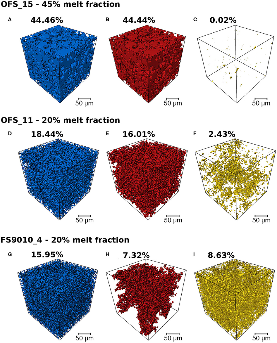
Figure 4. Variation in melt fraction connectivity between samples. The top row belongs to sample OFS-15 – subvolume 1. The middle row is sample OFS-11 – subvolume 2. The bottom row is sample FS9010-4 – subvolume 1. For each sample the total melt distribution is shown in blue (A,D,G), the connected melt distribution in red (B,E,H), and isolated melt distribution in yellow (C,F,I). The melt fraction listed on top of each panel is the bulk melt fraction in the sample, which can be different from the total melt fraction in each subvolume due to heterogeneous melt distribution during annealing. See the text in sections 2.3 and 4.1 for more discussions about the selection of subvolumes.

The step-like behavior of melt connectivity is revealed in the plots shown in Figure 5. The plot in Figure 5A shows the variation of the connected melt volume fraction as a function of the total melt volume fraction. The error bars in the plot indicate the uncertainty values derived by the method discussed in section 2.3. The broken line in the plot depicts 1:1 correlation. Data points falling on this line indicate that an insignificantly small portion of the melt is unconnected. As the plot shows, there is a sharp step-like deviation in the data points from the 1:1 correlation line around a total melt volume fraction of 0.17. The connected melt volume fraction assumes a zero value at melt fractions less than 0.14.

FIGURE 5

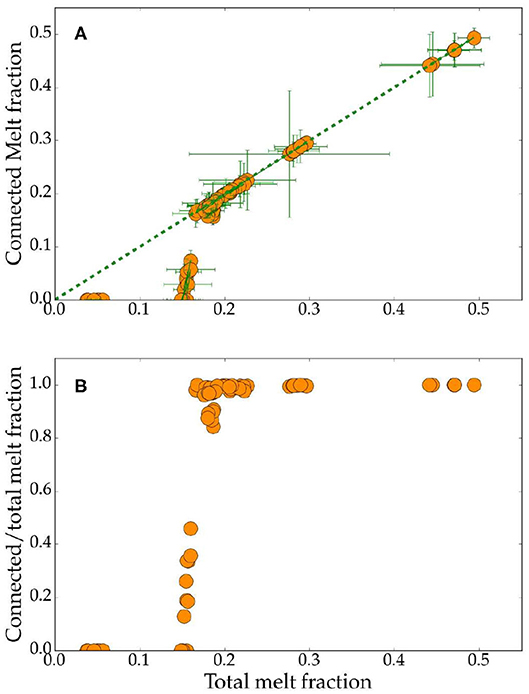
Figure 5. Plots of (A) connected melt volume fraction (B) ratio between connected and total melt volume fraction as a function of total melt volume fraction in all subvolumes. In (A), the dashed line indicates 1:1 correlation. Errorbars for melt volume fraction are given by the difference between automatically thresholded and manually thresholded melt fractions.

Melt connectivity involves three regimes, purely isolated, partially connected, and fully connected. These three regimes can be quantitatively defined by the ratio between connected and total melt volume fractions. The plot in Figure 5B shows the variation in this ratio as a function of the total melt volume fraction. The purely isolated regime, marked by zero connected melt fraction, is observed for total melt volume fractions ranging between 0 and 0.14. Between total melt volume fractions of 0.14 and 0.17, the connection threshold is established and the ratio increases rapidly from 0 to 1, with an increase in the total melt fraction. At total melt fractions above 0.17, the melt becomes fully connected, marked by the ratio of 1. Two important features of this data set are the establishment of a connection threshold at a total melt fraction of 0.14, a relatively high value, and the small width—only 3%—of the partially connected domain.

The step-like behavior of melt connectivity is not an artifact of image resolution for a number of reasons. First, the pixel size of 2D images, 0.325 μm, is substantially smaller than the grain sizes of the samples reported in Table 1. Additionally, the minimum pore size in our analyses, described next, is also substantially larger than the pixel size. Finally, the step-like transition in pore connectivity is a natural manifestation of pore geometry and is detected by other methods such as experimental determination of electrical conductivity and permeability (Mavko and Nur, 1997; Yoshino et al., 2003; Roberts et al., 2007; Bagdassarov et al., 2009a; Watson and Roberts, 2011; Thomson et al., 2019, 2020).

3.2. Pore and Throat Characteristics

Connectivity of individual pores—junctions in the network, joined by throats—are determined by the coordination number and the radius of these pores. In agreement with the increase in melt connectivity with the total melt fraction, these features also demonstrate a strongly non-linear variation with the increase in the melt fraction, as shown in Figures 6A,B.

FIGURE 6

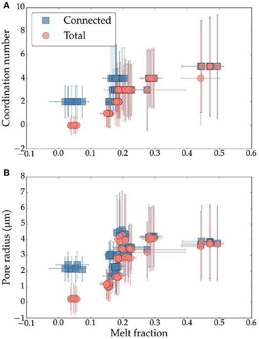
Figure 6. Plots of (A) median coordination number and (B) pore equivalent radius as a function of melt volume fraction in all subvolumes. The horizontal axis represents values of connected melt fraction for the filled squares and total melt fraction for filled circles. Error bars for melt volume fraction are given by the difference between automatically thresholded and manually thresholded melt fractions. Error bars for coordination number and pore radius are given by the standard deviation (1σ) of the measured values of pores.

The coordination number indicates the number of throats that are connected to an individual pore. Thus, a minimum coordination of 2 is necessary for a pore to be connected. The plot in Figure 6A shows the median coordination number of all pores from a subvolume as a function of melt fraction in that subvolume. The horizontal axis in the plot refers to total melt volume fraction for filled circles while it stands for connected melt volume fraction for the filled squares. The errorbars for PNM attributes in the vertical axes are calculated using one standard deviation. The errorbar in the horizontal axis of melt fraction is calculated using the method outlined in section 2.3. As the plot indicates, the two datasets diverge at melt fraction of 0.17. Below this threshold, the median coordination number shows a non-linear decrease with a decrease in the total melt fraction. In contrast, the median coordination number assumes a constant, minimum value of 2 for the connected melt volume fraction. This variation is also observed in pore network modeling of natural sandstones (Thomson et al., 2020). The increase in the coordination number with an increase in the total melt fraction, depicted by filled circles, indicates that the pores become more connected with an increase in the melt fraction. At melt volume fractions exceeding 0.4, the median coordination number assumes a constant value of 5, although the error bar, arising from the standard deviation, displays that pores with much higher and lower coordination numbers can coexist at such values. The large error bars at melt fractions above the full connection threshold, arising from a large range of connectivity in the pores, likely indicates some extent of surface tension-driven self segregation of large, well-connected pores draining melt out, and leaving behind smaller, unconnected pores (Hier-Majumder et al., 2006; King et al., 2011).

The median pore radius within each subvolume displays a behavior similar to the coordination number. The connection threshold is established only when the median pore radius is 2 μm or larger, as indicated by the filled-squares in Figure 6B. Smaller, submicron sized, and unconnected pores characterize the network at melt volume fractions below the connection threshold. The median pore radius increases up to a value of 5 μm for a melt volume fraction of 0.22. At higher melt volume fractions, the median pore radius gently decreases with an increase in the melt fraction, both for total and connected melts. This gentle decrease in the pore radius can arise from surface tension-driven self segregation, which is also supported by the increased range in coordination numbers at these melt fractions.

The variations in median throat length and radius with melt fraction are shown in Figures 7A,B. Unlike median pore diameter of total melt network, the median throat radius and length do not continually decrease to zero with a decrease in the melt fraction. Instead, these quantities become fixed at a minimum value with a decrease in the melt fraction beneath the establishment of the connectivity threshold at a total melt fraction of 0.14. In the melt-rich subvolumes, however, throat radius and throat length show a similar trend with melt fractions exceeding 0.22, as the pore radius. Overall, the throat radius in Figure 7A varies between a minimum value of 1μm and a maximum value of ~3μm, while the throat length varies within a range of 5 μm and 13 μm. It is worth noting that unlike the geometry of pores, the plots do not display a significant variation in the datasets for connected melt network (solid squares) and total melt network (solid circles).

FIGURE 7

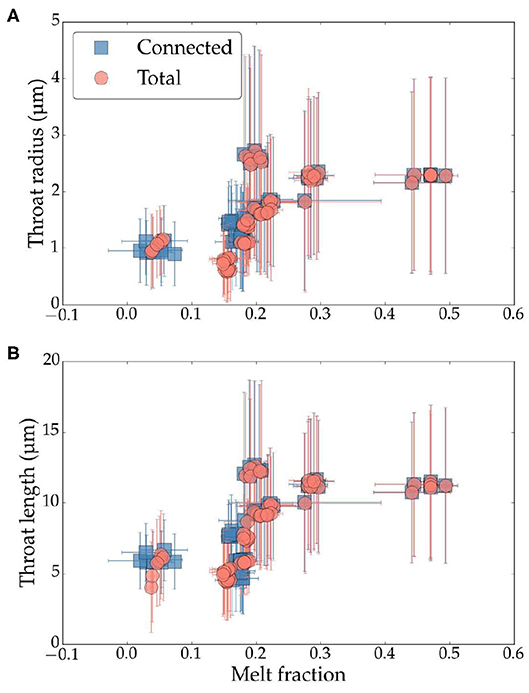
Figure 7. Plots of (A) median throat radius and (B) throat radius as a function of melt volume fraction in all subvolumes. The horizontal axis represents values of connected melt fraction for the filled squares and total melt fraction for filled circles. Error bars for melt volume fraction are given by the difference between automatically thresholded and manually thresholded melt fractions. Error bars for throat radius and lengths are given by the standard deviation (1σ) of the measured values.

4. Discussion

4.1. Selection of Subvolume

As discussed in section 2.2, we select subvolumes within the sample to calculate melt connectivity and to study the pore network. The selection of subvolume arises from two constraints. First, the computation time for pore network modeling becomes prohibitively large, when the analysis is carried over the entire sample. Selection of a suitable subvolume alleviates this issue. Second, the experimental samples are extremely heterogeneous with respect to the distribution of melt. This heterogeneity, likely arising from surface tension driven self segregation of the melt, can be observed in Figure 3. We manipulate these variations by manually selecting subvolumes that display uniform melt distribution within themselves, but can vary significantly from each other. This allows us to sample the variations in the melt volume fraction. Watson and Roberts (2011) follow a similar method of selecting subvolumes within the whole image to quantify Fe-FeS melt connectivity.

Besides the relatively uniform melt distribution it is also important to ensure that each subvolume contained sufficient number of grains, representing a statistically significant portion of the sample. For a subvolume V containing a total melt fraction ϕ, and an average grain size (diameter) d, the number of grains per subvolume is given by,

$\begin{array}{ll}n=\frac{24V(1-\varphi )}{4\pi d^3}.& (1)\end{array}$

We calculated this number of grains from each of our subvolumes, using the data reported in Table 1. We found that the median number of grains in each subvolume studied here was 10,530, a sufficiently large number to capture the grain scale variations. In contrast, the study by Watson and Roberts (2011) extracted subvolumes of 140–180 μm³. While this study did not report the grain size, the powder for synthetic aggregate was 45 μm, which might have grown to a larger size during annealing. Using a melt volume fraction of 0.15, a subvolume of 150 μm³, and a grain diameter of 45 μm in equation (1), we obtain an average of 60 grains per subvolume. While a direct comparison between these two different sets of subvolume are precluded by the lack of grain size data from Watson and Roberts (2011), this calculation indicates that our selection of subvolume is likely to incorporate a substantially larger number of grains than their subvolumes.

4.2. Comparison With Other Systems

Our results on the connection threshold agree well with previous experimental measurements of Bagdassarov et al. (2009a). In contrast, the connectivity threshold in olivine-FeS system measured by Watson and Roberts (2011) occurs at a lower melt fraction. The plot in Figure 8 outlines this distinction by comparing the fraction of connected melt volume as a function of total melt fraction in Figure 8A. Our data shows that the threshold, marked by non-zero value of the connected melt fraction, occurs at a total melt fraction of 0.14, compared to ~ 0.05 reported by Watson and Roberts (2011). While a similar discrepancy between the results of Bagdassarov et al. (2009a) and the results of Roberts et al. (2007) and Watson and Roberts (2011) have been discussed previously, a physical explanation, based on the development of microstructure during the annealing, remains elusive. In this section, we provide an explanation based on the theoretical models of surface-tension driven melt segregation during liquid phase sintering.

FIGURE 8

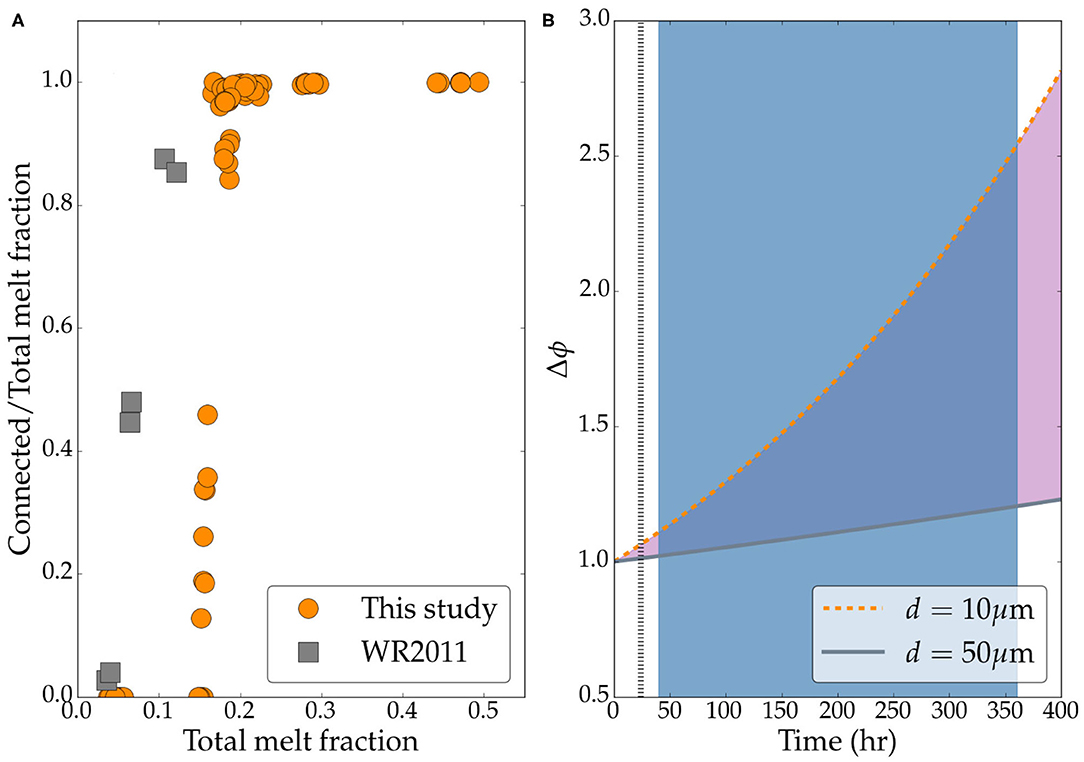
Figure 8. (A) Plot of connected melt fraction as a function of total melt fraction. The gray squares represent data digitally acquired from Figure 7 of Watson and Roberts (2011). Filled orange circles are data from this study. (B) Model prediction of melt enrichment by self segregation. The legends indicate the values of grain size used in calculating each curve. The vertical broken line marks 24 h, the duration of experiments in Watson and Roberts (2011), while the blue shaded area represents the duration of annealing for the samples used in this study. See text for more details on the model.

Non-wetting melts, characterized by a higher tension on the grain-melt interface compared to the grain-grain interface, self separate with time (Hier-Majumder et al., 2006). In the absence of deformation of the matrix, this process is described by the Thompson-Freundlich equation (Kingery et al., 1976, Ch. 9.4). This equation—sometimes used to calculate vapor pressure at curved solid interfaces—suggests that the chemical potential of components, such as Fe in the melt and olivine, are influenced by the surface tension, establishing a driving force for chemical dissolution and precipitation. In a theoretical study, Takei and Hier-Majumder (2009) posited that chemical dissolution and precipitation, assisted by tension at the curved grain-melt interface, can cause substantial transfer of melt. King et al. (2011) demonstrated that surface tension driven chemical dissolution-precipitation in olivine-basalt aggregates led to redistribution of the basaltic melt. In this model, the melt enrichment (for non-wetting melts) or depletion (for wetting melts) can be described by the enrichment factor,

$\begin{array}{ll}\Delta \varphi =\frac{\Delta {\varphi }_t}{\Delta {\varphi }_0},& (2)\end{array}$

where the numerator is the difference between maximum and minimum melt fractions at time t and the denominator is the difference between maximum and minimum melt fractions at the beginning of the annealing experiment. For non-wetting melts, the enrichment factor Δϕ increases above the value of unity with time, as more melt is segregated into isolated pockets. As a result, the melt fraction at which connection threshold is established, increases with time. This rate of increase, in the limit of linear perturbations can be expressed as

$\begin{array}{ll}\Delta \varphi ={\text{e}}^{\lambda t},& (3)\end{array}$

where λ is the growth rate and t is time. We present the calculation for growth rate in the Supplementary Material. Interested readers are referred to Takei and Hier-Majumder (2009) and King et al. (2011) for more details.

The result of this model, simulating surface tension driven melt enrichment, is shown in the plot in Figure 8B. In the plot, we show two curves, corresponding to two different grain sizes shown in the legend. The plot also outlines the duration of the experiment of Watson and Roberts (2011) as the broken vertical line and the range of annealing times of Solferino et al. (2015) and Solferino and Golabek (2018) as the shaded region. As the plot demonstrates, for a mean grain size of 10 microns, isolated pockets can be enriched by nearly a factor of 2.5 after 400 h. This rate is reduced for a larger grain size of 50 μm. Hence, the nearly factor of 3 higher connection threshold in the samples used in this study can be explained by the establishment of such isolated melt-rich pockets. While we observed evidence of stronger self segregation in our longer runs, due to the relatively similar grain size in our samples this contrast was more muted compared to the the contrast between our samples and the samples of Watson and Roberts (2011).

This explanation and our observations point to the fact that the connection threshold in experimental analogs of core forming materials depend both on the time of the experiments and the grain size. While Watson and Roberts (2011) did not characterize the grain size in their final experimental runs, their starting olivine grain size of 45 μm, is substantially larger than our grain sizes. As the plots indicate, a combination of the effect of larger grain size and shorter experimental duration suppressed self segregation of sulfide melts in their runs, leading to a lower threshold of connectivity. While the underlying assumption of linearity in the models precludes predictions over timescales of years, future studies combining long experiments, microtomographic studies, and numerical modeling of melt segregation can provide more robust estimates.

4.3. Melt Structure at Pinch-Off

The variations in pore and throat geometry with total melt fractions provides information about the relative distribution of pores and throat sizes at melt fractions below the connection threshold. The fact that throat radius and length assume a minimum value at a melt fraction of ~0.15, while the pore radius continues to decrease, indicates that the so-called “pinch-off” is not caused by drying out of the throats, as suggested by some previous numerical models (Wray, 1976; von Bargen and Waff, 1986; Wimert and Hier-Majumder, 2012). It is also commonly assumed that the pore network of non-wetting melts—such as the Fe-FeS melt in an olivine matrix—are characterized by isolated pores. Our results demonstrate a picture in the contrary. Instead, the pinch-off is marked by loss of pores that serve as junctions between the throats. In our samples, an isolated network is characterized by a collection stranded throats rather than a collection of isolated pores. This observation is consistent with the idea of “melt hysteresis” proposed by the numerical models of core forming melt network by Ghanbarzadeh et al. (2017).

4.4. Implications for Core Formation in Planetesimals

In this section, we focus on the implications of our results on segregation of core-forming liquids through a solid matrix. Cosmochemical evidence from Ureilites (Barrat et al., 2015; Budde et al., 2015) and iron meteorites (Kruijer et al., 2014) suggest that core seggregation in the parent bodies of these meteorites took place over a time scale of 1 Ma or less. The size of these planetesimal parent bodies could range between 1 km (de Pater and Lissauer, 2015, Chapter 12.5.2) up to larger bodies of 10% Earth mass (Rubie et al., 2011), leading to a range of acceleration due to gravitation. Assuming the density of the planetesimal is similar to the density of the Earth, we can scale the gravity by using Newton's law, g = (g_ER)/R_E, where the subscript E refers to the Earth.

The velocity, v, with which the dense, connected melt segregates can be expressed by Darcy's law,

$\begin{array}{ll}v=\frac{\Delta \rho gk}{\mu },& (4)\end{array}$

where Δρ is the density contrast between the melt and the solid, g is the gravity, k is the permeability, and μ is the viscosity of the sulfide melt. Following Watson and Roberts (2011), we use Δρ = 2000 kgm⁻³ and μ = 0.01 Pa s. We use the permeability results from (Ghanbarzadeh et al., 2017, Table S1) for a melt with a dihedral angle of 90^o embedded in a solid consisting of irregular grains with an average grain size d, yielding k = 5.94 × 10⁻³d²ϕ^2.53 m². Using these constants with a known radius of the planetesimal, we can calculate the melt percolation velocities at the connectivity threshold.

An important implication of our result is the high velocity of Fe-FeS melt segregation, as shown in Figure 9. Using the permeability from their microtmographic model Roberts et al. (2007, 2 × 10⁻¹⁵ m²) obtained a melt seggregation velocity of 1.5 cm/yr for a planetesimal of radius 100 km, too slow to explain the cosmochemical constraint of 0.5–1 Ma for core formation (Kruijer et al., 2014). Using a grain size of 50 μm, comparable to the powder size of their starting material, and the constants discussed above, we find that at the percolation threshold melt fraction of 0.14, core forming melts segregate with a velocity of 10.2 cm/yr. With this percolation velocity, a parcel of core forming melt can travel from the surface to the center of the 100 km planetesimal in 0.9 Ma, similar to the cosmochemical constraint (Kruijer et al., 2014).

FIGURE 9

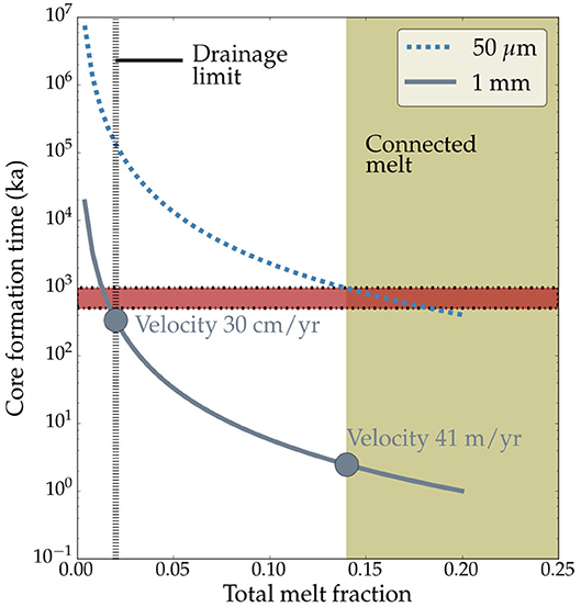
Figure 9. Core formation time in ka, defined as the time taken for a parcel of melt to travel from the surface to the center of a 100 km radius planetesimal, as a function of melt fraction. The legend indicates the grain size used to calculate the two curves. The vertical broken line is the drainage threshold from Ghanbarzadeh et al. (2017) and the horizontal shaded box indicates a time span of 0.5–1 Ma, the cosmochemical constraint on timing of core formation. The melt fractions above the connection threshold is indicated by the shaded region on the right of the plot. The two filled circles represent the time of core seggregation at the connection threshold and the drainage limit, respectively. The percolation velocities of core forming melts at these two values are annotated in the plot.

Despite the good agreement between this estimate and cosmochemical constraint on the timing of core formation in planetesimals, two factors need to be considered. First, the grain size in the planetesimals are larger, evidenced by the presence up to 10 mm diameter olivine grains in pallasites (Boesenberg et al., 2012). Using a grain size of 1 mm in our calculations, we find a percolation velocity of ~ 41 m/yr at the percolation threshold melt fraction of 0.14. At this percolation velocity, a parcel of melt will travel from the surface to the center of the planetesimal in only 2.5 ka. Second, the percolation velocity should decrease with time, as more melt is segregated into the core, reducing the permeability in a non-linear manner. Ghanbarzadeh et al. (2017) argue that during gravitational drainage, the melt hystersis effect allows continued drainage of melt well below the percolation threshold, down to a melt volume fraction of 0.02. Using this melt fraction and a grain size of 1mm, we calculate a percolation velocity of ~30 cm/yr. Since the melt becomes unable to drain further, we consider this velocity as the lower limit. Consequently, the time of 338 ka taken by a parcel of melt to travel from the surface to the center of the planetesimal with this velocity can be considered as an upper limit for the time of core segregation.

The high connection threshold in our samples does not imply that the Earth's mantle was left with 14 vol% stranded Fe-FeS melt following core formation for several reasons. First, as discussed above, once the connectivity is established, melt can continue to drain until a melt fraction of 0.02 remains trapped in the olivine matrix. While our study precludes direct confirmation of the results of this model, the near constant throat radius and length at melt fractions below the threshold shown in Figure 7, supports the general conclusion of melt hysteresis proposed by Ghanbarzadeh et al. (2017). Second, deformation of the interior of the planetesimal, a process absent in our samples annealed under a hydrostatic condition of stress, can create high permeability pathways and help drain stranded core forming melts (Rushmer et al., 2005; Groebner and Kohlstedt, 2006; Hustoft and Kohlstedt, 2006; Berg et al., 2017). Finally, during the process of Earth's accretion, collision between the planetesimals can generate sufficient heat to create a global magma ocean (Rubie, 2007; Rubie et al., 2011). The separation of metal and silicate within the magma ocean is no longer constrained by the connectivity threshold, as the liquid metal can be rapidly drained through the molten silicates (Stevenson, 1990; Elkins-Tanton et al., 2011).

5. Conclusions

• We identified three regimes of melt connectivity from our samples based on the fraction of connected melt and the total melt fraction. The connection threshold starts at around 14 vol% melt and full connectivity is established at around 17 vol% melt.

• The pore network model indicates that a minimum pore radius of 1.5–2μm and a coordination number of 2 is necessary for the establishment of a connected network.

• We suggest that the discrepancy between two contradicting estimates of Fe-FeS melt connection threshold can be explained by melt segregation driven by surface tension.

• Using our results of melt percolation threshold, we demonstrate that the core formation in planetesimals can take place in less than 500 ka.

Data Availability Statement

The datasets presented in this study can be found in online repositories. The names of the repository/repositories and accession number(s) can be found below: Sulfide pore network model results (https://royalholloway.figshare.com/articles/Sulfide_pore_network_model_results/12409394/1).

Author Contributions

P-RT carried out the image analysis and pore network modeling of all samples. GS provided the samples and carried out the X-ray microtomographic image acquisition. SH-M carried out the statistical analysis of the pore network model data. All authors contributed equally to the conceptualization and writing of the manuscript.

Funding

P-RT acknowledges support from a NERC Oil and Gas CDT graduate fellowship (grant number NE/M00578X/1).

Conflict of Interest

The authors declare that the research was conducted in the absence of any commercial or financial relationships that could be construed as a potential conflict of interest.

Acknowledgments

GS acknowledges support from Christian Liebske (ETH Zurich) and Federica Marone (PSI Villigen, beamline TOMCAT) for preparation of samples and acquisition of tomographies, respectively.

Supplementary Material

The Supplementary Material for this article can be found online at: https://www.frontiersin.org/articles/10.3389/feart.2020.00339/full#supplementary-material Supplemental data from the pore network analysis are provided through the Figshare repository (Hier-Majumder et al., 2020).

References

Abe, Y. (1997). Thermal and chemical evolution of the terrestrial magma ocean. Phys. Earth Planet. Interiors 100, 27–39. doi: 10.1016/S0031-9201(96)03229-3

CrossRef Full Text | Google Scholar

Bagdassarov, N., Golabek, G. J., Solferino, G., and Schmidt, M. W. (2009a). Constraints on the Fe-S melt connectivity in mantle silicates from electrical impedance measurements. Phys. Earth Planet. Interiors 177, 139–146. doi: 10.1016/j.pepi.2009.08.003

CrossRef Full Text | Google Scholar

Bagdassarov, N., Solferino, G., Golabek, G. J., and Schmidt, M. W. (2009b). Centrifuge assisted percolation of Fe-S melts in partially molten peridotite: time constraints for planetary core formation. Earth Planet. Sci. Lett. 288, 84–95. doi: 10.1016/j.epsl.2009.09.010

CrossRef Full Text | Google Scholar

Barrat, J. A., Rouxel, O., Wang, K., Moynier, F., Yamaguchi, A., Bischoff, A., et al. (2015). Early stages of core segregation recorded by Fe isotopes in an asteroidal mantle. Earth Planet. Sci. Lett. 419, 93–100. doi: 10.1016/j.epsl.2015.03.026

CrossRef Full Text | Google Scholar

Berg, C. F., Lopez, O., and Berland, H. (2017). Industrial applications of digital rock technology. J. Petrol. Sci. Eng. 157, 131–147. doi: 10.1016/j.petrol.2017.06.074

CrossRef Full Text | Google Scholar

Blunt, M. J. (2017). Multiphase Flow in Permeable Media: A Pore-Scale Perspective. Cambridge: Cambridge University Press. doi: 10.1017/9781316145098

CrossRef Full Text

Boesenberg, J. S., Delaney, J. S., and Hewins, R. H. (2012). A petrological and chemical reexamination of Main Group pallasite formation. Geochim. Cosmochim. Acta 89, 134–158. doi: 10.1016/j.gca.2012.04.037

CrossRef Full Text | Google Scholar

Buades, A., Coll, B., and Morel, J. (2005). “A non-local algorithm for image denoising,” in 2005 IEEE Computer Society Conference on Computer Vision and Pattern Recognition (CVPR'05), Vol. 2 (San Diego, CA), 60–65. doi: 10.1109/CVPR.2005.38

CrossRef Full Text | Google Scholar

Buades, A., Coll, B., and Morel, J.-M. (2008). Nonlocal image and movie denoising. Int. J. Comput. Vis. 76, 123–139. doi: 10.1007/s11263-007-0052-1

CrossRef Full Text | Google Scholar

Budde, G., Kruijer, T. S., Fischer-Gödde, M., Irving, A. J., and Kleine, T. (2015). Planetesimal differentiation revealed by the Hf-W systematics of ureilites. Earth Planet. Sci. Lett. 430, 316–325. doi: 10.1016/j.epsl.2015.08.034

CrossRef Full Text | Google Scholar

de Pater, I., and Lissauer, J. J. (2015). Planetary Sciences. Cambridge: Cambridge University Press.

Duncan, M. S., Schmerr, N. C., Bertka, C. M., and Fei, Y. (2018). Extending the solidus for a model iron-rich martian mantle composition to 25 GPa. Geophys. Res. Lett. 45, 10211–10220. doi: 10.1029/2018GL078182

CrossRef Full Text | Google Scholar

Elkins-Tanton, L. T. (2012). Magma oceans in the inner solar system. Annu. Rev. Earth Planet. Sci. 40, 113–139. doi: 10.1146/annurev-earth-042711-105503

CrossRef Full Text | Google Scholar

Elkins-Tanton, L. T., Weiss, B. P., and Zuber, M. T. (2011). Chondrites as samples of differentiated planetesimals. Earth Planet. Sci. Lett. 305, 1–10. doi: 10.1016/j.epsl.2011.03.010

CrossRef Full Text | Google Scholar

Faul, U. H., and Scott, D. (2006). Grain growth in partially molten olivine aggregates. Contribut. Mineral. Petrol. 151, 101–111. doi: 10.1007/s00410-005-0048-1

CrossRef Full Text | Google Scholar

German, R. M. (2013). Liquid Phase Sintering. New York, NY: Springer US. Available online at: https://books.google.co.uk/books?id=PE72BwAAQBAJ.

Google Scholar

Ghanbarzadeh, S., Hesse, M. A., and Prodanović, M. (2017). Percolative core formation in planetesimals enabled by hysteresis in metal connectivity. Proc. Natl. Acad. Sci. U.S.A. 114, 13406–13411. doi: 10.1073/pnas.1707580114

PubMed Abstract | CrossRef Full Text | Google Scholar

Groebner, N., and Kohlstedt, D. L. (2006). Deformation-induced metal melt networks in silicates: implications for core-mantle interactions in planetary bodies. Earth Planet. Sci. Lett. 245, 571–580. doi: 10.1016/j.epsl.2006.03.029

CrossRef Full Text | Google Scholar

Hier-Majumder, S., and Hirschmann, M. M. (2017). The origin of volatiles in the Earth's mantle. Geochem. Geophys. Geosyst. 18, 1–12. doi: 10.1002/2017GC006937

CrossRef Full Text | Google Scholar

Hier-Majumder, S., Ricard, Y., and Bercovici, D. (2006). Role of grain boundaries in magma migration and storage. Earth Planet. Sci. Lett. 248, 735–749. doi: 10.1016/j.epsl.2006.06.015

CrossRef Full Text | Google Scholar

Hier-Majumder, S., Solferino, G., and Thomson, P.-R. (2020). Sulfide Pore Network Model Results. doi: 10.17637/rh.12409394.v1. Available online at: https://royalholloway.figshare.com/articles/dataset/Sulfide_pore_network_model_results/12409394

CrossRef Full Text

Hirschmann, M. M. (2000). Mantle solidus: experimental constraints and the effects of peridotite composition. Geochem. Geophys. Geosyst. 1. doi: 10.1029/2000GC000070

CrossRef Full Text | Google Scholar

Hustoft, J. W., and Kohlstedt, D. L. (2006). Metal-silicate segregation in deforming dunitic rocks. Geochem. Geophys. Geosyst. 7, 1–11. doi: 10.1029/2005GC001048

CrossRef Full Text | Google Scholar

Iassonov, P., Gebrenegus, T., and Tuller, M. (2009). Segmentation of x-ray computed tomography images of porous materials: a crucial step for characterization and quantitative analysis of pore structures. Water Resour. Res. 45:W09415. doi: 10.1029/2009WR008087

CrossRef Full Text | Google Scholar

Ketcham, R. A., and Carlson, W. D. (2001). Acquisition, optimization and interpretation of x-ray computed tomographic imagery: applications to the geosciences. Comput. Geosci. 27:381–400. doi: 10.1016/S0098-3004(00)00116-3

CrossRef Full Text | Google Scholar

King, D. S. H., Hier-Majumder, S., and Kohlstedt, D. L. (2011). An experimental study of the effects of surface tension in homogenizing perturbations in melt fraction. Earth Planet. Sci. Lett. 307, 735–749. doi: 10.1016/j.epsl.2011.05.009

CrossRef Full Text | Google Scholar

Kingery, W. D., Uhlmann, D. R., and Bowen, H. K. (1976). Introduction to Ceramics, 2nd Edn. New York, NY: Wiley.

Google Scholar

Kruijer, T. S., Touboul, M., Fischer-Gödde, M., Bermingham, K. R., Walker, R. J., and Kleine, T. (2014). Protracted core formation and rapid accretion of protoplanets. Science 344, 1150–1154. doi: 10.1126/science.1251766

PubMed Abstract | CrossRef Full Text | Google Scholar

Mavko, G., and Nur, A. (1997). The effect of a percolation threshold in the Kozeny-Carman relation. Geophysics 62, 1480–1482. doi: 10.1190/1.1444251

CrossRef Full Text | Google Scholar

Minarik, B. (2003). The core of planet formation. Nature 422, 126–128. doi: 10.1038/422126a

PubMed Abstract | CrossRef Full Text | Google Scholar

Otsu, N. (1979). A threshold selection method from gray-level histograms. IEEE Trans. Syst. Man Cybernet. 9, 62–66. doi: 10.1109/TSMC.1979.4310076

CrossRef Full Text | Google Scholar

Paganin, D., Mayo, S. C., Gureyev, T. E., Miller, P. R., and Wilkins, S. W. (2002). Simultaneous phase and amplitude extraction from a single defocused image of a homogeneous object. J. Microsc. 206, 33–40. doi: 10.1046/j.1365-2818.2002.01010.x

PubMed Abstract | CrossRef Full Text | Google Scholar

Pal, N. R., and Pal, S. K. (1993). A review on image segmentation techniques. Pattern Recogn. 26, 1277–1294. doi: 10.1016/0031-3203(93)90135-J

CrossRef Full Text | Google Scholar

Roberts, J. J., Kinney, J. H., Siebert, J., and Ryerson, F. J. (2007). Fe-Ni-S melt permeability in olivine: implications for planetary core formation. Geophys. Res. Lett. 34, 1–5. doi: 10.1029/2007GL030497

CrossRef Full Text | Google Scholar

Rubie, D. C. (2007). “Formation of Earth's core,” in Treatise on Geophysics, ed Schubert, G., (Amsterdam: Elsevier), 51–90. doi: 10.1016/B978-044452748-6.00140-1

CrossRef Full Text | Google Scholar

Rubie, D. C., Frost, D. J., Mann, U., Asahara, Y., Nimmo, F., Tsuno, K., et al. (2011). Heterogeneous accretion, composition and core-mantle differentiation of the Earth. Earth Planet. Sci. Lett. 301, 31–42. doi: 10.1016/j.epsl.2010.11.030

CrossRef Full Text | Google Scholar

Rushmer, T., Petford, N., Humayun, M., and Campbell, A. J. (2005). Fe-liquid segregation in deforming planetesimals: coupling core-forming compositions with transport phenomena. Earth Planet. Sci. Lett. 239, 185–202. doi: 10.1016/j.epsl.2005.08.006

CrossRef Full Text | Google Scholar

Rushmer, T., and Watson, H. C. (2015). How to make a planet: an introduction. Am. Mineral. 100, 1093–1097. doi: 10.2138/am-2015-5205

CrossRef Full Text | Google Scholar

Ryzhenko, B., and Kennedy, G. C. (1973). The effect of pressure on the eutectic in the system Fe-FeS. Am. J. Sci. 273, 803–810. doi: 10.2475/ajs.273.9.803

CrossRef Full Text | Google Scholar

Schluter, S., Sheppard, A., Brown, K., and Wildenschild, D. (2014). Water resources research grants. Water Resour. Res. 50, 3615–3639. doi: 10.1002/2014WR015256

CrossRef Full Text

Sezgin, M., and Sankur, B. (2004). Survey over image thresholding techniques and quantitative performance evaluation. J. Electron. Imaging 13, 146–166. doi: 10.1117/1.1631315

CrossRef Full Text | Google Scholar

Solferino, G. F., and Golabek, G. J. (2018). Olivine grain growth in partially molten Fe–Ni–S: a proxy for the genesis of pallasite meteorites. Earth Planet. Sci. Lett. 504, 38–52. doi: 10.1016/j.epsl.2018.09.027

CrossRef Full Text | Google Scholar

Solferino, G. F., Golabek, G. J., Nimmo, F., and Schmidt, M. W. (2015). Fast grain growth of olivine in liquid Fe-S and the formation of pallasites with rounded olivine grains. Geochim. Cosmochim. Acta 162, 259–275. doi: 10.1016/j.gca.2015.04.020

CrossRef Full Text | Google Scholar

Solomatov, V. S. (2000). “Fluid dynamics of a terrestrial magma ocean,” in Origin of the Earth and Moon (Tuscon, AZ: The University of Arizona Press), 323–338.

Google Scholar

Solomatov, V. S., and Stevenson, D. J. (1993). Suspension in convective layers and style of differentiation of a terrestrial magma ocean. J. Geophys. Res. 98, 5375–5390. doi: 10.1029/92JE02948

CrossRef Full Text | Google Scholar

Stevenson, D. J. (1990). “Fluid dynamics of core formation,” in Origin of the Earth (New York, NY), 231–249. doi: 10.1016/0040-1951(90)90103-F

PubMed Abstract | CrossRef Full Text

Takei, Y., and Hier-Majumder, S. (2009). A generalized formulation of interfacial tension driven fluid migration with dissolution/precipitation. Earth Planet. Sci. Lett. 288, 138–148. doi: 10.1016/j.epsl.2009.09.016

CrossRef Full Text | Google Scholar

Thomson, P.-R., Aituar-zhakupova, A., and Hier-majumder, S. (2018). Image segmentation and analysis of pore network geometry in two natural sandstones. Front. Earth Sci. 6:58. doi: 10.3389/feart.2018.00058

CrossRef Full Text | Google Scholar

Thomson, P.-R., Hazel, A., and Hier-Majumder, S. (2019). The influence of microporous cements on the pore network geometry of natural sedimentary rocks. Front. Earth Sci. 7:48. doi: 10.3389/feart.2019.00048

CrossRef Full Text | Google Scholar

Thomson, P.-R., Jefferd, M., Clark, B. L., Chiarella, D., Mitchell, T., and Hier-Majumder, S. (2020). Pore network analysis of brae formation sandstone, North Sea. Mar. Petrol. Geol.

Google Scholar

Tonks, W. B., and Melosh, H. J. (1990). “The physics of crystal settling and suspension in a turbulent magma ocean,” in Origin of the Earth, eds Newsom, H. E., and Jones, J. H., (New York, NY: Oxford University Press), 151–174.

Google Scholar

Trier, Ø. D., and Jain, A. K. (1995). Goal-directed evaluation of binarization methods. IEEE Trans. Pattern Anal. Mach. Intell. 12, 1191–1201. doi: 10.1109/34.476511

CrossRef Full Text | Google Scholar

von Bargen, N., and Waff, H. (1986). Permeabilities, interfacial areas and curvatures of partially molten systems: results of numerical computations of equilibrium microstructures. J. Geophys. Res. 91, 9261–9276. doi: 10.1029/JB091iB09p09261

CrossRef Full Text | Google Scholar

Watson, H. C., and Roberts, J. J. (2011). Connectivity of core forming melts: experimental constraints from electrical conductivity and X-ray tomography. Phys. Earth Planet. Interiors 186, 172–182. doi: 10.1016/j.pepi.2011.03.009

CrossRef Full Text | Google Scholar

Weiss, B. P., and Elkins-Tanton, L. T. (2013). Differentiated planetesimals and the parent bodies of chondrites. Annu. Rev. Earth Planet. Sci. 41, 529–560. doi: 10.1146/annurev-earth-040610-133520

CrossRef Full Text | Google Scholar

Wildenschild, D., Vaz, C., Rivers, M., Rikard, D., and Christensen, B. (2002). Using x-ray computed tomography in hydrology: systems, resolutions, and limitations. J. Hydrol. 267, 285–297. doi: 10.1016/S0022-1694(02)00157-9

CrossRef Full Text | Google Scholar

Wimert, J. T., and Hier-Majumder, S. (2012). A three-dimensional microgeodynamic model of melt geometry in the earth's deep interior. J. Geophys. Res. Solid Earth 117:B04203. doi: 10.1029/2011JB009012

CrossRef Full Text | Google Scholar

Wray, P. J. (1976). The geometry of two-phase aggregates in which the shape of the second phase is determined by its dihedral angle. Acta Metall. 24, 125–135. doi: 10.1016/0001-6160(76)90015-8

CrossRef Full Text | Google Scholar

Yoshino, T., Walter, M. J., and Katsura, T. (2003). Core formation in planetesimals triggered by permeable flow. Nature 422, 154–157. doi: 10.1038/nature01459

PubMed Abstract | CrossRef Full Text | Google Scholar

Youssef, S., Rosenberg, E., Gland, N., Kenter, J., Skalinski, M., and Vizika, O. (2007). High resolution CT and pore-network models to assess petrophyscial properties of homogeneous and heterogeneous carbonates. Society of Petroleum Engineers. doi: 10.2118/111427-MS

CrossRef Full Text | Google Scholar