 Andrea Andrisaniand
 Francesco Vespe
95% of researchers rate our articles as excellent or good
Learn more about the work of our research integrity team to safeguard the quality of each article we publish.
Find out more
ORIGINAL RESEARCH article
Front. Earth Sci. , 02 October 2020
Sec. Atmospheric Science
Volume 8 - 2020 | https://doi.org/10.3389/feart.2020.00320
This article is part of the Research Topic GNSS and InSAR Meteorology View all 4 articles
We performed some refinements to the Boundary Profile eValuation (BPV) method, developed by Vespe and collaborators (Vespe et al., 2004; Vespe and Persia, 2006; Vespe, 2016), for the retrieval of vertical atmospheric humidity profiles from Radio Occultation (RO) observations. Previous BPV models solve typical rank deficiencies in treating RO data by recurring to parametric dry atmospheric refractivity models, such as the Hopfield or the CIRA86aQ. The involved parameters were selected by fitting observed RO Bending Angles (BAs) in the stratosphere where humidity is negligible. Total refractivity was then obtained from the observed BAs via a variational method. Such approach furnishes a valid alternative to the usual Abel inversion. Humidity profiles were finally achieved by subtracting dry refractivity contribution to the total refractivity. Nevertheless, unphysical behaviors of “negative” values of humidity can occur when the dry refractivity profiles are extrapolated toward the lower part of the troposphere. In order to avoid such unphysical behavior, in this work we recur to a second fitting for the total refractivity data, through a Least Square Error (LSE) method having a non-negative residual constraint. This is mathematically achieved with a modification of the usual LSE functional to minimize, by means of an additional exponential fast increasing term with respect to negative residuals. A Levenberg-Marquardt method relative to this new functional has been developed too, in order to numerically estimates the relative minimizers. With this approach, new dry refractivity profiles, more suited to be extrapolated in the troposphere, are recovered. We tested this new method with a series of almost 450 of GPS-RO observations from the FORMOSAT-3 COSMIC-1 Space Mission in 2009. The results show that unphysical negative values for partial water vapor pressures are removed, without losing, but in most cases even improving, the accuracy of the retrieved values, as compared with data from the European Centre for Medium-Range Weather Forecasts (ECMWF) and the National Centers for Environmental Prediction (NCEP) meteorological analysis, the Constellation Observing System for Meteorology, Ionosphere, and Climate (COSMIC) data analysis, and as the RAwinsonde Observation (RAOB) balloons excursions suggest.
Global Navigation Satellite System Radio Occultation (GNSS-RO) observations have provided in the last 20 years a huge amount of data suitable to perform global change studies and operational meteorology on global range (Jin et al., 2012; Bauer et al., 2015). By treating RO observations with specific techniques, real time information about atmospheric refractivity vertical profiles can be achieved (Fjeldbo and Eshleman, 1969; Fjeldbo et al., 1971; Kursinski et al., 1997). One of the main drawbacks in the atmospheric sensing by means of RO observations lies in a rank deficiency problem in deriving the most important atmospheric parameters, that is, pressure, temperature and humidity concentrations, from refractivity data alone. In order to resolve this problem with three unknown, only two equations are actually available: (1) the Smith & Weintraub microwave refractivity equation (Smith and Weintraub, 1953), and (2) a thermodynamic state equation in hydrostatic equilibrium, both reported in section How to Retrieve Thermodynamic Profiles for the Troposphere.
This rank deficiency is usually solved by merging observations with models in “simple” or “direct” fashion (Gorbunov and Sokolovskiy, 1993) or by applying 1DVAR (NDVAR) techniques (Healy and Heyre, 2000). Following Kursinski's classification (Kursinski and Kursinski, 2013), simple models recover humidity profiles by determining dry refractivity first and then operate a simple subtraction from the total refractivity achieved by RO observations. Dry refractivity can be estimated through external information, as temperature profiles (Kursinski et al., 2000; Kursinski and Hajj, 2001), or other GPS data (Ge et al., 2001; Pacione et al., 2001), or by a priori atmospheric models (Vespe et al., 2004; Vespe and Persia, 2006). 1DVAR or NDVAR techniques consist in an optimization procedure, using background data, forward models and the related covariance error matrices to statistically match atmospheric state profiles with observations (Eyre, 1994; Healy and Heyre, 2000). The cost function to minimize is usually given in this form:
Here, y stays for the observed data, while x is the data to be recovered. In absence of errors and uncertainties we have y = H (x), that is, H is the forward model linking the vector variable x to the vector observation y. Rank deficiency occurs because H gradient is often given by a horizontal rectangular matrix. In order to reduce the spread of the possible solutions that minimize J, it is also required that x doesn't deviate too much from some previous, a priori information, represented by the background vector xB. So, a second squared term is added in the expression of J. Deviations from background data and observed data are then weighted, respectively, by the reciprocals of the expected background covariance error matrix (B) and of the sum of the expected covariance error matrices due to observations (E) and forward model (F). In the case of ROs, y may represent atmospheric refractivity or rawer experimental data such as BAs or excess Doppler shifts (Kuo et al., 2000) (we describe these quantities in section Radio Occultation Observations). Various comparative studies (Zou et al., 2000; Cucurull and Derber, 2013; Gorbunov et al., 2019), have shown that BAs assimilation should be preferred. A lot of efforts is nowadays dedicated to a correct estimation of the error covariance matrices, in particular to error propagation from RO experimental observations to thermodynamic atmospheric data (Schwarz et al., 2017, 2018; Li et al., 2019; Innerkofler et al., 2020); however the main sources of errors in 1DVAR method result in the uncertainty in background data (Cucurull and Derber, 2013). Finally, dimension number N usually indicate how many spatial-temporal parameters are used to describe the RO event. In the 1-dimensional case, ROs are described in terms of elevations, in the hypothesis of a spherical symmetric atmosphere; for a more detailed description of the event, such as in numerical weather prediction forecasting, multidimensional variation is needed. This increases the complexity of the required background model, and a considerable mole of data are to be treated, with high computational cost. For this reason, mixed procedures are often adopted (Gorbunov et al., 2019).
The Boundary Profile eValuation (BPV) method (Vespe et al., 2004; Vespe and Persia, 2006) can be considered as a simple model, even if it avoids the use of external information. The BPV works in two aspect: (1) it retrieves total refractivity profiles from bending angles (BA)s data without recurring to the Abel transform (see section How to Retrieve Total Refractivity Profiles), but by applying instead a variational method; (2) it retrieves wet refractivity profiles—that is, refractivity due to the presence of water vapor—in a simple model fashion. This last step is performed by considering RO observations that involve only the stratosphere and the upper part of the troposphere, where humidity concentration is negligible. In this way, an accurate recovering of wet refractivity profiles by GNSS-RO observations alone is possible. Nevertheless, it does not avoid seldom-negative unphysical estimates about wet pressure, as most of the simple models.
In the present work, we developed some refinements to the BPV method in order to avoid such unphysical behaviors. By imposing a non-negative constraint for the residuals of the fitting procedure, we assure a non-negative range for wet refractivity values. Our work differs from Vespe (2016) in two aspects: (1) total refractivity is now the physical quantity to fit, in place of the BA; (2) a penalty method approach (Smith and Coit, 1996), based on a modification of the functional usually employed to minimize in the Least Square Error (LSE) method, is adopted.
The article is structured as follows. In section Radio Occultation Observations and The BPV Approach we expose a brief review about RO observations and the BPV method. In section LSE Method With a Non-negative Residuals Constraint we describe in detail the mathematical scheme used to perform the non-negative residual constrained fitting. In section Discussion of the Results we apply the new method to a sample of almost 450 GNSS-RO observations from the COSMIC-1 mission. Finally, in section Conclusions we comment the obtained results.
RO observations primarily consist in tracking and measuring short wave radio signal arriving at a receiver from a transmitter during an occultation phase, occurring when one or both the receiver and the transmitter are falling behind/emerging from a planet or more generally a celestial body with atmosphere. During an occultation, ray lines of the electromagnetic field cross different layers—at different altitudes—of the celestial body atmosphere, whose physical properties and chemical compositions sensibly affect radio signal phases and intensities as registered at the receiver point. By applying opportune inversion techniques, from the time trends of the measured phases and intensities it is possible to trace profiles of the physical/chemical properties of the planet atmosphere. The whole RO observation thus results in a scanning process of the atmosphere.
On Earth a RO observation is usually performed by a satellite from a GNSS constellation—often a GPS one—playing the role of the transmitter, whose emitted signals are detected by a Low Earth Orbit (LEO) satellite, having a GNSS signal receiver mounted on it (Figure 1). LEO-LEO ROs, involving signals at different bands with respect to the L-band of the GPS, are often considered too (Kirchengast and Hoeg, 2004; Benzon and Høeg, 2016). This investigation method for the Earth's atmosphere was first suggested in some works of 1960s (Fishbach, 1965; Lusignan et al., 1969). However, radio occultation concept was initially applied to the remote sounding of Mars and Venus atmospheres, through the Mariner and Pioneer space missions (Fjeldbo and Eshleman, 1969; Fjeldbo et al., 1971; Kliore and Patel, 1982), and successively to outer planets as well, with the Voyager missions (Lindal, 1991). Only with the advent of the GPS constellation, together with the launch of several LEO satellites, it was achieved the needed Earth global coverage in order to enhance the existing atmospheric data by RO observations (Yunck et al., 1988).
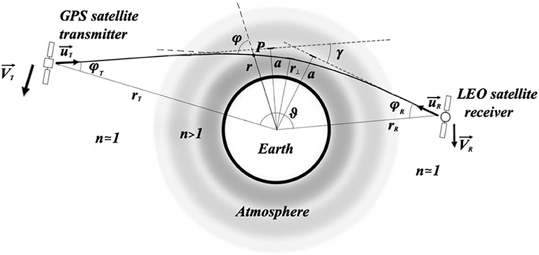
Figure 1. Graphical representation of a RO observation. A radio signal path starting from the GPS transmitter T deviates from the straight line by a BA γ toward the LEO receiver R, due to the refraction of the atmosphere. Impact parameter is denoted by a, whereas φ is the incident angle of the ray line on the spherical surface of constant refraction index n. BA γ and impact parameter a are estimated by Doppler shifts measurements of the carrier frequency, if satellites positions and velocities, respectively , and , , are known.
Radio wave occultations by a celestial body with atmosphere mainly result in an excess of the Doppler shift of signal frequency. This excess, with respect to the usual Doppler shift observed in vacuum when the transmitter and the receiver are in relative motion, is due to the deflection of the ray lines connecting the two satellites from the straight line path, as a consequence of the atmospheric refraction as schematically depicted in Figure 1 (Fjeldbo et al., 1971; Kursinski et al., 1997). Because the local atmospheric refraction index depends on its (local) pressure, temperature and chemical decomposition, it is possible to achieve some information about these quantities from bending angles measurements.
The basic approach in bending angles retrievals from Doppler shift measurements make use of the Geometric Optics (GO) approximation. By assuming a spherically symmetric distribution for the atmosphere, Snell's refraction law results in the Bouguer's formula (Born and Wolf, 1970)
where φ is the incident angle of the ray signal at a point P of the terrestrial atmosphere with distance r from the Earth's center (Figure 1), whereas n (r) is the refraction index for that distance. The parameter a, known as the impact parameter, is a constant of the ray path: in geometrical terms, it represents the distance of closest approach in the absence of any bending.
At the transmitter T and at the receiver R, where n ≃ 1, we have the following relationships
From Figure 1, we can see that the angles φT and φR are related with the BA γ by
where ϑ is the angular distance between the two satellites, as seen from the Earth's center.
In the classical approximation of the Doppler effect—i.e., by neglecting the relativistic terms –carrier frequencies of the GPS signals arriving at the LEO satellite fR are subjected to the following variations with respect to the original frequencies fT:
where , are, respectively, the transmitter and the receiver satellite velocities, while , are the departing and incoming radio signal directions. Observe that in vacuum, , with the unit vector connecting the transmitter with the receiver; in this case (4) becomes
that is, the usual Doppler formula. So, by subtracting (5) from (4), we obtain the pure atmospheric contribution to the measured Doppler effect (Fjeldbo and Eshleman, 1969).
By considering the radial and the transverse components of and , Equation (4) can be rewritten as
By measuring Doppler shift Δf by a time differentiation of the incoming signal phase at the receiver (Kursinski et al., 1997), Equations (6) and (2) give us the impact parameter a in terms of the known positions rT, rR and velocities , of the GPS and LEO satellites. Bending angles γ are then given by (3) as functions of a, being the angle ϑ also known from satellites positions.
Hypothesis of isotropic atmosphere can be slightly weakened by assuming a local spherical symmetry around the point of tangent propagation for the ray path (Figure 1), because the main contribution to the total BA γ comes from this area, usually having a horizontal extension of 200–300 km (Kursinski et al., 1997). In this case, distances are to be measured with respect to the local symmetry center, determined for example by local center of curvature of the Earth WGS84 ellipsoid, or even of the Geoid, which accurately models the Earth shape. In general, BAs defined by Equation (3) are often denoted as the effective BAs (Gorbunov et al., 2019), to be distinguished from the real BAs when atmospheric spherical symmetry is not verified.
The approach described so far, based on GO approximation, actually works for ray deviations taking place in the upper part of the stratosphere. For radio signal sounding the lower stratosphere and the troposphere, Equation (6) is no more suited. Indeed, the more complex structures of these atmospheric layers determine a spreading of wave-lengths, with the resulting multipath effects, that is, the simultaneous arrival of multiple radio waves along different ray paths, causing phase signals to change with a very irregular pattern in time. This effect is particular evident in the lower troposphere, where water vapor concentrations are not negligible. In order to resolve most of the multipath ambiguity and to recover BAs under such conditions, a more detailed analysis of the measured phase and amplitude signal, based for example on the wave optic approximation (Sokolowskiy, 2001; Gorbunov, 2002; Jensen et al., 2003; Gorbunov and Lauritsen, 2004; Gorbunov and Kirchengast, 2015), is required. Nevertheless, residual multipath effects due to atmospheric anisotropy are more challenging to treat, because they cannot be resolved by most of the methods mentioned above.
Ray signals approaching the planet with a given impact parameter a during an occultation are belt by an angle γ(a) due to the atmospheric refraction. Such angle can be retrieved by the refraction index profile n (r) of a spherical symmetric atmosphere in the following way. The Snell's law in a differential form reads:
where the (differential) BA dγ is defined as the difference between incidence angle φ in Equation (7) and refraction angle. By developing the term on the right of (7) in a Taylor expansion up to the first order, we get
By (1), we can rewrite (8) as
and by integrating (9) between rtop and r⊥, respectively the radius of the top of the atmosphere, beyond which n ≃ 1, and the distance of the ray path tangent point (φ = π/2) from the Earth's center (Figure 1), we get half of the total BA γ. So
Observe that the integrand function is correctly defined for r > r⊥, since rn (r) > rn (r) sin φ = a, while it has a (usually integrable) singularity at the extreme r = r⊥, being r⊥n (r⊥) = a.
BPV method is a useful technique able to retrieve both total refractivity profiles and the atmospheric wet content as well, without requiring additional information apart from bending angles and impact parameters data derived from GNSS RO observations. A dry atmospheric model for the refractivity, such as the Hopfield (Hopfield, 1969) or the CIRA86aQ (Kirchengast and Poetzi, 1999) is required in order to estimate such quantities.
In order to retrieve n (r) from (10), one often applies an inversion formula. By operating a change of variable r → x = rn (r) inside the integral on the right of Equation (10), we get:
where (x) = n (r (x)). Formula (11) gives the ratio as the Abel transform (Bracewell, 1965) of the function g
If g (x)x goes to zero when x → ∞, we can apply the inverse Abel transform in order to retrieve g from the bending angles γ(a):
Once obtained the function g (x), one gets (x) by inverting (12) and successively sets n (r) = (x) for .
Formula (13) presents some drawbacks when applied to real cases. Firstly, neglecting actual (local) deviations from refractivity spherical symmetry can results in negative artifacts error (Ahmad and Tyler, 1998). A more important source of error which occurs even in the symmetric case is due to the presence of waveguides, that is, layers of atmosphere inside which short wave radio signals are trapped in, usually located at tropical latitudes, just above oceanic surfaces. From a mathematical point of view, big lapses of humidity at ~2 km of altitude above these zones cause a sharp decrease of the refractive index profile, and when , i.e., in case of super-refraction (Sokolovskiy, 2003), the refractive radius x = rn (r) is no more monotone. As a consequence, the function (x) is now multivalued, each ramification giving rise to the same bending angle profile. From a deeper analysis (Sokolovskiy, 2003; Gorbunov et al., 2019), refractivity profiles recovered by Abel inversion (13) are actually under-estimated below this super-refraction quote.
An alternative approach for the inversion problem of (10), which can take into account super-refraction effects, is the BPV method as exposed in Vespe and Persia (2006). It uses variational techniques in order to approach the actual refractivity n (r) from a first guess n0(r). A scheme of the various steps followed by this technique is showed in Figure 2.
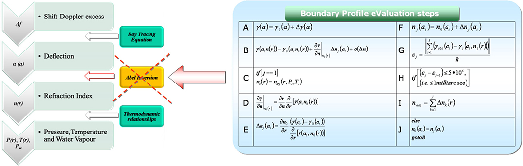
Figure 2. A schematic description of the variational approach used by the BPV method in order to retrieve total refractivity. More details can be found in Vespe and Persia (2006).
Variational techniques often need a good starting point n0, in order to work well. Such choice is retrieved by recurring to parametric dry refractivity models. Hopfield or CIRA86aQ models, the last one actually a background model but here used as a parametric function, has been considered. The Hopfield model relates refractivity, defined as N = 106(n − 1), to the altitude h = r − RE, where RE is the Earth radius, by means of the pressure P0 and the temperature T0 at the surface of the considered location. It reads
with α1 = 77.6 K/mbar, whereas . The CIRA86aQ is given in tabular form: the mapping terms latitude and the month of the year are used as parameters.
Once chosen a dry refraction model ndry(r; α, β), the parameters (α, β) are selected by fitting the observed BAs with the BAs obtained by inserting the dry profiles ndry(r; α, β) in (1), limited to those ray paths scanning atmospheric regions where water vapor concentrations are negligible. This usually happens in the stratosphere and in those layers of the troposphere where temperatures are lower than 250 K (Kursinski et al., 1997). This fitting is performed with an LSE method, with the numerical solution (α0, β0) achieved by means of a Levenberg-Marquardt algorithm (Nocedal and Wright, 2006). The starting point for the variational iterative algorithm of Figure 2 is then set to n0(r) = ndry(r; α0, β0). In order to take into account of possible super-refraction effects, an additional bump term, localized in the lower troposphere, can be added to n0(r). Indeed, starting from a region of over-estimated refractivity, by a variational method we can approach the right local minimum without incurring in the Abel retrieved local minimum, which lies in a region of under-estimation.
By neglecting compressibility effects on the gaseous of the atmosphere, air refractivity in the microwave spectra is related to thermodynamic parameters by the following equation:
where T is the temperature in Kelvin, Pdry, Pwet are the partial pressures, respectively, of the dry air and water vapor in mbar, ne is the electron number density per cubic meter, f is the frequency of the electromagnetic signal in Hertz, whereas W and I are, respectively, the liquid water droplets and ice aerosol content in grams per cubic meter. The first term is due to the induced polarization of the air molecules, the second and the third ones, respectively, to the permanent and the induced polarization of the water molecules, the fourth one is the contribute due to the free electrons mainly in the ionosphere, whereas the remaining two are aerosol scattering terms. The first two terms correspond to the original Smith and Weintraub equation; the third term coefficient is that reported in Thayer (1974), whereas the fourth term coefficient is taken from Papas (1965). For the scattering coefficients we refer to Kursinski (1997).
As we can see from (14), atmospheric dispersion is only due to the ionosphere in the microwave region. By using a linear combination of the bending angles from both the L1 and L2 GPS signals, the ionospheric contribution can be removed (Vorob'ev and Krasil'nikova, 1994; Kursinski et al., 1997). So, total refractivity, as estimated from this linear combination of BAs, does not contain the fourth term. Besides, for realistic concentrations of liquid and ice aerosols, the scattering terms can be neglected too (Kursinski et al., 1997). Equation (14) can then be rewritten as:
By comparing Ndry–the term inside the first square brackets on the right of (15)—with the ideal state equation for the dry air
we obtain the following relationship between air density ρdry, measured in kg m−3, and Ndry:
where is the mass per mole of the dry air, and R = 8.313 J (kg mol)−1 is the universal gas constant. If we take now the hydrostatic equation for the dry air
by inserting (17) in (18) and by integrating (18), we obtain another equation among thermodynamic quantities and refractivity terms:
Here href is a reference altitude with a known value of the partial pressure for dry air. By placing Ndry = Ntot − Nwet and by replacing Nwet with the terms inside the second square brackets on the right of (15), we can rewrite (19) together with (15) in form of the following system:
Obviously, such a system cannot be solved, since we have just two equations for the three unknowns Pdry, Pwet and T, as previously stated.
In order to invert (20), some additional information about Ndry have to be achieved. A first estimation of the dry refraction index profiles is given by extrapolating ndry (r; α0, β0), recovered in the previous step for the estimation of the refractivity in the stratosphere and in the higher part of the troposphere, toward the lower tropospheric regions. So, we set
At this point we can obtain Pdry by (19), once set Pdry(href). In a previous version of the BPV model (Vespe, 2016), href = h250 K, i.e., the altitude at which T = 250 K, while Pdry(h250 K) was given by RAOB data. Here, in order to make the model self-sustained, we set href = htop, with htop defined as the higher altitude at which we can estimate Ndry, whereas Pdry(h250 K) is set equal to zero. Such a simple choice is motivated by the fact that htop lies on the higher layers of the stratosphere, reaching a quote of 60 km. Besides, errors due to upper boundary approximations decrease exponentially at lower altitude (Kursinski et al., 1997), so that they can be neglected in investigating the troposphere as in the present work.
Once estimated dry pressure profiles, temperatures for the tropospheric region can be obtained by the Smith and Weintraub formula for the dry refractivity, i.e., the first term on the right of (15),
Finally, we get the wet pressure profile by the wet refractivity profile Nwet(h) = Ntot(h) − Ndry(h)
The thermodynamic profiles estimated by means of Equations (19), (22) and (23) are quite accurate (Vespe et al., 2004); nevertheless, for what concerns Equation (23), it does not avoid the occurrences of negative wet pressures, as can be shown in Figure 3 and in Figures 5, 6 of section Discussion of the Results. This is essentially due to negative values of wet refractivity that may happen by applying formula (21), when we extrapolate the dry refractivity profile down to the tropospheric region.
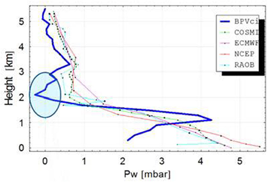
Figure 3. A typical unphysical behavior of the wet pressure profiles by the previous BPV model. The negative value of the wet pressure is emphasized by the cyan circle.
In order to avoid these negatives values, we need a better estimation of the dry refractivity profile, in particular more suited to be extrapolated toward the troposphere. We achieve this by fitting again the total refractivity profile Ntot(h) with the theoretical curves of the parametric refractivity models such as the Hopfield or the CIRA86aQ, but by imposing this time a non-negative constraint about the residuals Δn (r) = n (r) − ndry(r; α, β), limited to the troposphere and the lower layers of the stratosphere.
Details about the mathematical method employed to perform such task is reported in section LSE Method With a Non-Negative Residuals Constraint. Observe that our present work differentiates from what done in Vespe (2016), since the constrained LSE fit is now computed on the total refractivity data rather than on the BA profiles. Once the new optimal parameters (α1, β1) are retrieved, by inserting them in the first equation of (21) in place of (α0, β0), we can avoid all the negative wet pressures occurrences. Besides, as we will see in Section 5, we acquire a general improvement in the humidity profile estimation, when compared with some experimental data.
In this section, we describe a possible approach for the particular constrained LSE problem exposed at the end of the subsection How to Retrieve Thermodynamic Profiles for the Troposphere, by using a penalty method (Smith and Coit, 1996). Let y = f (α; x) to be a physical quantity depending on the variable x by means of a parametric function f with parameters α = (α1, α2, .., αN). A set of n measured values xi and yi, i = 1, .., n, is given for x and y. We want to find the optimal parameters α* such that the following conditions are achieved:
1. Some or all the residuals have to be non-negative, or at least , with dy > 0. The quantity −dy denotes an allowed minimal negative residue, fixed for example by the experimental uncertainties in evaluating y.
2. Once verified condition 1, fitting for some or all the data yi by means of has to be minimal in the LSE sense.
In Vespe (2016), a LSE method verifying conditions 1 and 2 was achieved by applying a weighting scheme. Here we expose another approach, that take into account a different function to minimize with respect to the quadratic one used in the ordinary LSE method:
with no conditions to be applied on the parameters α. The quantity λ is positive. About σ1,i and σ2,i, they assume the values 1 or 0, respectively, if the i-th data yi has to be fitted or not, or if the if the i-th residual Δyi has to be positive or not. In the following, we will consider the simplest case σ1,i = σ2,i = 1 for every i, being the general case easily recoverable from this.
Observe that Fλ in (24) is actually given by the sum of the function F used in the usual LSE problems
plus a penalty function (Smith and Coit, 1996) given by a series of exponential terms, with the residuals Δyi = yi − f (α; xi), multiplied by a factor −λ, as exponents. The value of λ in (24) has to be chosen very large. Indeed, as λ goes to infinity,
where
So, if minimizes F∞ –i.e., makes F∞finite – no negative residuals can exist. On the other end, as long as the Δyi terms are positive, F∞ = F and the residuals are minimized according to the usual LSE method. Therefore, for high values of λ, we can take as a good approximation of , which solves the ideal case as described in points 1 and 2. Indeed, working directly with F∞ –or even starting with Fλ for very large values of λ–is not convenient from a computational point of view, treating this function with infinities or extremely high quantities when Δyi ≫ 1/λ. We have followed this iterative method:
I Find the optimal parameter for the usual LSE problem, that is, the minimizer for the function F of Equation (25). Then set .
II Fixed a value k > 1, define a sequence (λj)1 ≤ j ≤ J, with and λj+1 = kλj.
III Defined , with the i-th residual at the j-th cycle, and given M the maximal number allowed by the numerical computing environment (for MATLAB environment M ~ e603), if > ln(M), than replace λj+1 with .
IV Find the minimizer of Fλj, using the minimizer of the previous step as starting point. For the first step set .
The algorithm then stops at λ = λJ, when residuals are greater than the allowed negative quantity -dy.
For a given value of λ, we have applied the Levenberg-Marquardt algorithm in order to find the minimizer of (24). Being this method usually adopted for functions of the type F as in (25) (Nocedal and Wright, 2006), we briefly describe how we can adapt it to Fλ.
Denoted by δ the increment of α, by applying a first order development of the Taylor series to f we get , so that
Then, for the gradient of Fλ(α + δ) with respect to δ we have
By imposing ∇δFλ(α + δ) = 0, we get
where
Finally, we add the typical Levenberg-Marquardt's damping term to the first factor on the right of (26), so that (26) becomes
with β a non-negative value.
We tested our method with 2009 GPS-RO data from FORMOSAT-3 COSMIC-1 Space Mission. Approximately 450 RO observations were considered, regarding middle latitudes and tropics. Refractivity profiles, together with pressure, wet pressure and temperature profiles, were retrieved by solely using BAs and impact parameters observed data. We made a comparison with the previous BPV method without the second constrained fitting, together with other models as well. In particular, we considered ECMWF and NCEP meteorological analysis, COSMIC data analysis, and we compare all of them with the RAOB data, derived by balloons excursions.
In estimating dry refractivity profiles from the total refractivity ones, water vapor concentrations result in positive bias with respect to the real value. This justifies the application of the constrained fitting as described in section LSE Method With a Non-negative Residuals Constraint. In particular, we adopted the following scheme about the coefficients σ1,i, σ2,i in (24):
I We performed the usual fitting of the total refractivity profile by means of dry refractivity curves for altitudes far above the 250 K quote. With reference of Equation (24), we set σ1,i = 1, σ2,i = 0 when hi ≳ hT = 250 K + Δh, being Δh a given height. We suppose that, at these quotes, water vapor contribution is negligible compared to the other sources of error for the dry refractivity.
II We performed a fitting with a non-negative-residuals constraint—σ1,i = 1, σ2,i = 1–for altitudes hT = 250 K ≲ hi ≲ hT = 250 K + Δh, that is, when water vapor refractivity is one of the main sources of error for the dry refractivity.
III We just imposed a non-negative residuals constraint—σ1,i = 0, σ2,i = 1–for altitudes hi ≲ hT = 250 K, that is, when water vapor refractivity is comparable with dry refractivity, so that total refractivity cannot be fitted by a dry refractivity model.
We remember that the BPV method, as exposed in Vespe et al. (2004), just applies the usual LSE fitting for altitudes h ≳ hT = 250 K.
The critical altitude hT = 250 K was achieved by formula (22), with the assumption that Ndry(h) = Ntot(h) as long as the temperature T (h) is <250 K. The quote where T = 250 K is achieved for the last time was set as the quote. We repeated again this procedure up to convergence: few cycles are usually required. For what concerns Δh, the extension of this transition regions, is still a matter of study, together with its optimal location. By some empirical evidence we choose Δh = 5 km; further researches will be required in order to better define it.
In Figures 4, 5, we report some examples for the estimated profiles, at tropical and middle latitudes, respectively. The elevations hT = 250 K and hT = 250 K + Δh, as achieved with the constrained fitting, are reported with horizontal dash lines in the refractivity profile figures (the hT = 250 K elevations, as obtained by the ordinary fitting, was omitted). In Figure 5, we can see how the negative values occurrences for the wet pressure, as acquired by the previous BPV method with the Hopfield model, are corrected by the refinements introduced in this work. Unphysical behaviors are less frequent with the CIRA86aQ; nevertheless, they are corrected too with this new version of the BPV method, as we can see in Figure 6.
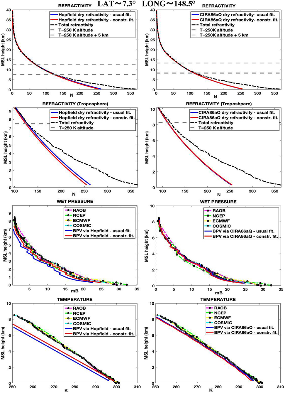
Figure 4. Refractivity, tropospheric refractivity, wet pressure and temperature profiles for a near-equatorial location. The graphs are obtained by the BPV and the previous BPV method without the second constrained fitting, for both the Hopfield (left) and CIRA86aQ (right) dry refractivity models. ECMWF, NCEP, COSMIC, and RAOB profiles are also reported for comparison.
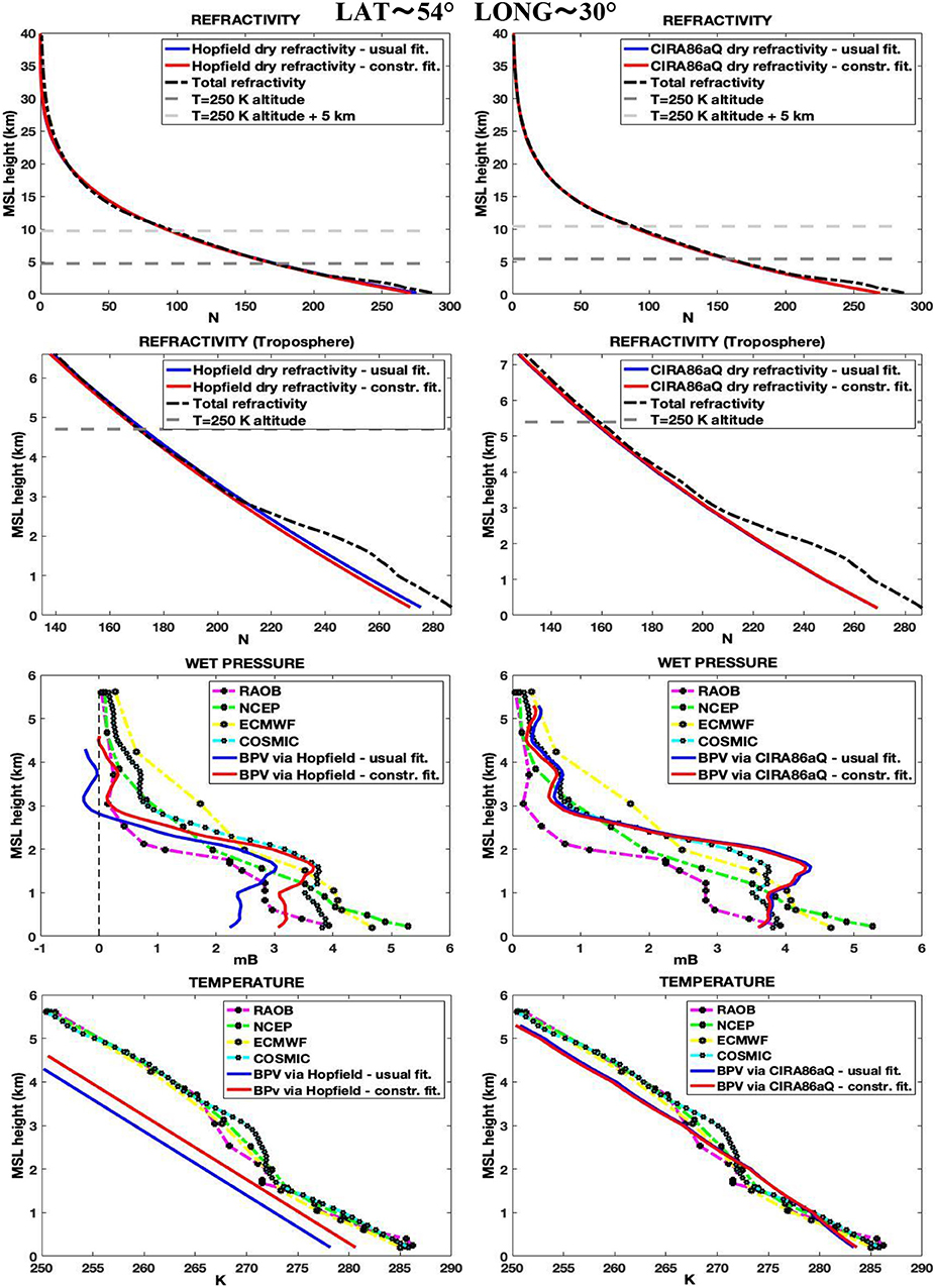
Figure 5. Profiles of the same quantities of the previous figure, for a middle latitude location. About the wet pressure with the Hopfield model, we observe that the unphysical behavior for the profile recovered by the previous BPV method is corrected with the second constrained fitting.
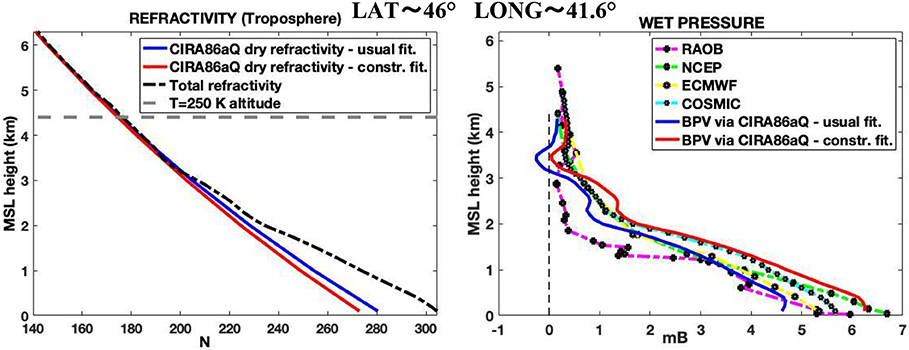
Figure 6. Even if less frequently with respect to the Hopfield model, wet pressure negative values may occur with the CIRA85aQ as well. In this case too, negative values disappear when the second constrained fitting is applied.
In Figures 7–9, detailed statistical studies about BPV wet pressures deviation from RAOB data, concerning, respectively, northern middle latitudes, tropics and southern middle latitude, are reported. Polar zones, with low concentrations of water vapor, were not considered. For what concerns data quality control, we limit ourselves to reject all those wet pressure values <-0.01 mB. The number of the remaining data, for each elevation, is reported at the bottom of Figures 7–9. As one can see, even more than 50% of the data can be lost in some cases, if a constrained fitting method is not adopted. On the contrary, no data were rejected when the constrain was applied. Data loss is more evident with the Hopfield's model, for all the latitudes. This is an expected result, since the CIRA86aQ model.is considered more reliable than the Hopfield one in estimating the dry refractivity of the atmosphere.
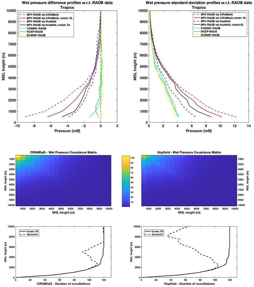
Figure 7. Top: Difference (left) and standard deviation (right) profiles for the wet pressure at Tropics, with respect to the RAOB values. Middle: Covariance error matrices for the constrained CIRA86aQ case (left) and the constrained Hopfield case (right). Bottom: Number of RO observations considered, in both the constrained and unconstrained case, for the CIRA86aQ (left), and the Hopfield (right).
Boundary Profile eValuation models and techniques perform differently at varying latitudes. For the tropics, the CIRA86aQ model improves when the positive residual constrains are applied (Figure 7, upper left and right). On the contrary, Hopfield model works better without such conditions. For the northern middle latitudes, constrained CIRA86aQ estimations are more biased with respect to the unconstrained ones; nevertheless, they are less scattered, as one can see on the top-right of Figure 8. Again, the contrary happens for the Hopfield model. Finally, for the southern middle latitudes (Figure 9), the constrained case seems to work better for both the models. This odd behavior between the constrained-unconstrained cases may be explaining by noting that, the greater the number of the rejected data, the better the unconstrained models perform (compare the graphs at the top and the bottom of Figures 7–9). So, better performances occurring sometime for the unconstrained case, may be actually due to a higher quality of the data samples, with respect to those used in the constrained case.
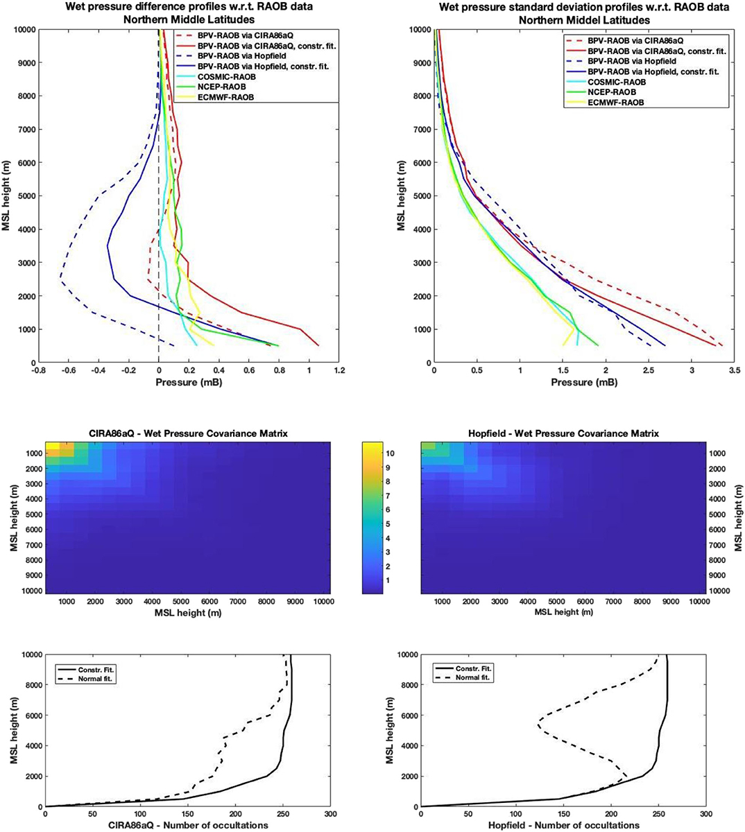
Figure 8. Top: Difference (left) and standard deviation (right) profiles for the wet pressure at Northern Middle Latitudes, with respect to the RAOB values. Middle: Covariance error matrices for the constrained CIRA86aQ case (left) and the constrained Hopfield case (right). Bottom: Number of RO observations considered, in both the constrained and unconstrained case, for the CIRA86aQ (left), and the Hopfield (right).
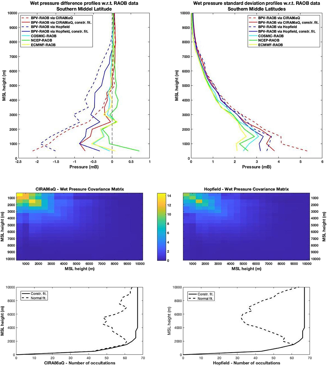
Figure 9. Top: Difference (left) and standard deviation (right) profiles for the wet pressure data at Southern Middle Latitudes, with respect to the RAOB values. Middle: Covariance error matrices for the constrained CIRA86aQ case (left) and the constrained Hopfield case (right). Bottom: Number of RO observations considered, in both the constrained and unconstrained case, for the CIRA86aQ (left), and the Hopfield (right).
Hopfield model seems to work better than the CIRA86aQ both at the tropics and at the northern hemisphere, in this last case just for altitude lower than 2.5 km. In the southern hemisphere differences among the two model are not relevant. On the other end, the CIRA86aQ model is less biased at northern latitudes for altitudes above 2.5 Km. In general, quadratic deviation from the RAOB data are smaller for the Hopfield model, as one can check by the covariance matrix errors reported in the middle of Figures 7–9. The fact that the Hopfield model works better than the CIRA86aQ may be due to some biased errors, both for the model and for the BPV “simple fashion” approach in estimating wet profiles, that compensate each other.
By comparing the BPV results with data by NCEP, ECMWF and COSMIC, we can immediately verify that the firsts are not accurate as the latter ones. BPV wet pressure values are in general under-estimated with respect to the RAOB data, in particular for the tropics and for altitudes below 5 km; this determines higher values of quadratic deviations as well. Nevertheless, for southern latitudes, BPV values obtained by the constrained fitting are of comparable accuracy with respect to those from NCEP, EWMCF, and COSMIC.
This study confirms the role of the BPV method as a stand-alone technique, capable of provide accurate atmospheric profiles of important thermodynamic quantities from GPS-RO observations. With the constrained fitting, as described in section 4, we avoid negative humidity. In particular, losses of more than 50% of the available data can be recovered. As we can see by the difference profiles on the top-left corner of Figures 7–9, the constrained fitting determines a general overestimation of the wet profiles with respect to the previous BPV. Yet the standard deviations graphs on the top-right corner of Figures 7–9 show that this overestimation in most cases does not affect the overall quality of the recovered profiles.
Further improvements are needed to the BPV model in order to reduce the gap with respect to other meteorological data source such as the NCEP and the ECMWF ones, together with COSMIC as well, all of these making use of 1DVAR or NDVAR approaches. In particular, we have to consider other options for what concerns rules I, II and III as reported in section Discussion of the Results, in order to better define the threshold altitude above which humidity is essentially absent, and maybe a more refined thermodynamic description could be needed too.
Besides, we believe that BPV results could be assimilated in a 1DVAR algorithm in which background data are obtained with the approach described in this work. Future studies will be dedicated to this task.
The raw data supporting the conclusions of this article will be made available by the authors, without undue reservation.
All authors listed have made a substantial, direct and intellectual contribution to the work, and approved it for publication.
This research was carried out in the framework of the project Advanced EO Technologies for studying Climate Change impacts on the environment– OT4CLIMA which was funded by the Italian Ministry of Education, University and Research (D.D. 2261 del 6.9.2018, PON R&I 2014-2020 e FSC).
AA was employed by the company EOG GmbH.
The remaining author declares that the research was conducted in the absence of any commercial or financial relationships that could be construed as a potential conflict of interest.
Ahmad, B., and Tyler, G. L. (1998). The two-dimensional resolution kernel associated with retrieval of ionospheric and atmospheric refractivity profiles by Abelian inversion of radio occultation phase data. Radio Sci. 33, 129–142. doi: 10.1029/97RS02762
Bauer, P., Thorpe, A., and Brunet, G. (2015). The quiet revolution of numerical weather prediction. Nature 525, 47–55. doi: 10.1038/nature14956
Benzon, H.-H., and Høeg, P. (2016). Wave optics based LEO-LEO radio occultation retrieval. Radio Sci. 51, 589–602. doi: 10.1002/2015RS005852
Cucurull, L. C. J., and Derber, P. R. J. (2013). A bending angle forward operator for global positioning system radio occultation. J. Geophys. Res. Atmos. 118, 14–28. doi: 10.1029/2012JD017782
Eyre, J. R. (1994). Assimilation of Radio Occultation Measurements Into a Numerical Weather Prediction System. ECMWF Technical Memoranda, 199.
Fishbach, F. F. (1965). A satellite method for temperature and pressure below 24 km. Bull. Am. Meteorol. Soc. 9, 528–532. doi: 10.1175/1520-0477-46.9.528
Fjeldbo, G., and Eshleman, V. R. (1969). The atmosphere of Venus as studied with the Mariner 5 dual radio-frequency occultation experiments. Radio Sci. 4, 879–897. doi: 10.1029/RS004i010p00879
Fjeldbo, G., Kliore, A. J., and Eshleman, V. R. (1971). The neutral atmosphere of Venus as studied with the Mariner V radio occultation experiments. Astron. J. 76, 123–140. doi: 10.1086/111096
Ge, S., Shum, C. K., Zhao, C. Y., Gutman, S., and Hocke, K. (2001). “GPS limb-sounding retrieval of water vapor using ground based network and spaceborne data,” in IAG 2001 Scintific Assembly (Budapest).
Gorbunov, M., Stefanescu, R., Irisov, V., and Zupanski, D. (2019). Variational assimilation of radio occultation observations into numerical weather prediction models: equations, strategies and algorithms. Remote Sens. 11:2886. doi: 10.3390/rs11242886
Gorbunov, M. E. (2002). Canonical transform method for processing radio occultation data in the lower troposphere. Radio Sci. 37, 9-1–9-10. doi: 10.1029/2000RS002592
Gorbunov, M. E., and Kirchengast, G. (2015). Uncertainty propagation through wave optics retrieval of bending angles from GPS radio occultation: theory and simulation results. Radio Sci. 50, 1086–1096. doi: 10.1002/2015RS005730
Gorbunov, M. E., and Lauritsen, K. B. (2004). Analysis of wave fields by Fourier integral operators and their application for radio occultations. Radio Sci. 39:RS4010. doi: 10.1029/2003RS002971
Gorbunov, M. E., and Sokolovskiy, S. V. (1993). Remote Sensing of Refractivity from Space for Global Observation of Atmospheric Parameters. Max Planck Institute for Meteorology Report, 119.
Healy, G., and Heyre, J. (2000). Retrieving temperature, water vapor and surface pressure information from refractive index profiles derived by radio occultations: a simulation study. Quart. J. Roy. Mateorol. Soc. 126, 1661–1683. doi: 10.1256/smsqj.56606
Hopfield, H. S. (1969). Two-quartic tropospheric refractivity profile for correcting satellie data. J. Geophys. Res. 74, 4487–4499. doi: 10.1029/JC074i018p04487
Innerkofler, J., Kirchengast, G., Schwarz, M., Pock, C., Jäggi, A., Andres, Y., et al. (2020). Precise orbit determinarion for climate applications of GNSS radio occultation including uncertainty estimation. Remote Sens. 12:1180 doi: 10.3390/rs12071180
Jensen, A. S., Lohmann, L. S., Benzon, H.-H., and Nielsen, A. S. (2003). Full spectrum inversion of radio occultation signals. Radio Sci. 38:1040. doi: 10.1029/2002RS002763
Jin, S. G., Feng, G. P., and Gleason, S. (2012). Remote Sensing Using GNSS Signals: Current Status and Future Directions. GPS Solutions.
Kirchengast, G., and Hoeg, P. (2004). “The ACE+ mission: an atmosphere and climate explorer based on GPS, GALILEO, and LEO-LEO radio occultation,” in Occultations for Probing Atmosphere and Climate (Berlin; Heidelberg: Springer).
Kirchengast, H. G. J., and Poetzi, W. (1999). The CIRA86aQ UoG Model: Amazon.Comn extEnsion of the CIRA-86 monthly Tables Including Humidity Tables and a Fortran95 Global Moist Air Climatology Model. ESA/estec No. 8/1999.
Kliore, A. J., and Patel, I. R. (1982). Thermal structure of the atmosphere of Venus from Pioneer Venus radio occutations. Icarus 52, 320–334. doi: 10.1016/0019-1035(82)90115-4
Kuo, Y. H., Sokolovskiy, S. V., Anthes, R. A., and Vandenberghe, F. (2000). Assimilation of GPS radio occultation data for numerical weather prediction. Terr. Atmos. Ocean. Sci. 11, 157–186. doi: 10.3319/TAO.2000.11.1.157(COSMIC)
Kursinski, E. R. (1997). The GPS radio occultation concept: theoretical performance and initial results [Ph. D. thesis]. California Institute of Technology, Pasadena, CA, United States.
Kursinski, E. R., and Hajj, G. A. (2001). A comparison of water vapor derived from GPS occultations and global wheather analysis. J. Geophys. Res. 106, 1113–1138. doi: 10.1029/2000JD900421
Kursinski, E. R., Hajj, G. A., Schofield, J. T., Linfield, R. P., and Hardy, K. R. (1997). Observing Earth's atmosphere with radio occulation measurements using Global Positioning System. J. Geophys. Res. 102, 23429–23465. doi: 10.1029/97JD01569
Kursinski, E. R., and Kursinski, A. (2013). “How well do we understand the low latitude, free tropospheric water vapor distribution?” in FORMOSAT-3/COSMIC Data Users Workshop 2011, (Taipeh).
Kursinski, R. E., Hajj, G. A., Leroy, S. S., and Herman, B. (2000). The GPS radio occultation technique. TAO 11, 53–114. doi: 10.3319/TAO.2000.11.1.53(COSMIC)
Li, Y., Kirchengast, G., Scherllin-Pirscher, B., Schwaerz, M., Nielsen, J. K., Ho, S., et al. (2019). A new algorithm for the retrieval of atmospheric profiles from GNSS radio occultation in moist air and comparisonn to 1DVar retrievals. Remote Sens. 11:2729. doi: 10.3390/rs11232729
Lindal, G. F. (1991). The atmosphere of Neptune: an analysis of radio occultation data acquired with Voyager 2. Astron. J. 103, 967–982. doi: 10.1086/116119
Lusignan, B., Modrell, G., Morrison, A., Pomalaza, J., and Ungar, S. G. (1969). Sensing the Earth's atmosphere with occulation satellites. Proc. IEEE 4, 458–467. doi: 10.1109/PROC.1969.7000
Pacione, R., Sciarretta, C., Faccani, C., Ferretti, R., and Vespe, F. (2001). GPS PW assimilation into MM% with the nudging technique. Phys. Chem. Earth 26, 481–485. doi: 10.1016/S1464-1895(01)00088-6
Schwarz, J., Kirchengast, G., and Schwaerz, M. (2017). Integrating uncertainty propagation in GNSS radio occultation retrieval:From bending angle to dry-air atmospheric profiles. Earth Space Sci. 4, 200–228. doi: 10.1002/2016EA000234
Schwarz, J., Kirchengast, G., and Schwaerz, M. (2018). Intregrating uncertainty propagation in GNSS radio occultation retrieval: from excess phase to atmospheric bending angle profiles. Atmos. Meas. Tech. 11, 111–125. doi: 10.5194/amt-11-111-2018
Smith, A. E., and Coit, D. W. (1996). “Constraint handling techniques – penalty functions, section C 5.2,” in Handbook of Evolutionary Computation (Oxford: Oxford University Press and Institute of Physics Publishing).
Smith, E. K., and Weintraub, S. (1953). The constants in the equation for atmospheric refractive index at radio frequancies. Proc. IRE 41, 1035–1037. doi: 10.1109/JRPROC.1953.274297
Sokolovskiy, S. (2003). Effect of superrifraction on inversions of radio occultation signals in lower troposphere. Radio Sci. 38:1058. doi: 10.1029/2002RS002728
Sokolowskiy, S. (2001). Modeling and inverting radio occultation signals in the moist troposphere. Radio Sci. 36, 441–458. doi: 10.1029/1999RS002273
Thayer, G. D. (1974). An improved equation for the radio refractive index of air. Radio Sci. 9, 803–807. doi: 10.1029/RS009i010p00803
Vespe, F. (2016). “Retrieval of atmospheric humidity profiles from GNSS radio occultation observations,” in 67-th International Astronautical Congress (Guadalajara).
Vespe, F., Benedetto, C., and Pacione, R. (2004). The use of refractivity retrieved by radio occultation technique for the derivation of atmospheric water vapor content. Phys. Chem. Earth 29, 257–266. doi: 10.1016/j.pce.2004.01.004
Vespe, F., and Persia, T. (2006). Derivation of the water vapor content from GNSS radio occulations observations. J. Atmos. Oceanic Technol. 23, 936–943. doi: 10.1175/JTECH1891.1
Vorob'ev, V. V., and Krasil'nikova, T. G. (1994). Estimation of the accuracy of the atmospheric refractive index recovery from Doppler shift measurements at frequencies used in the NAVSTAR system. Phys. Atmos. Ocean 29, 602–609.
Yunck, T. P., Lindal, G. F., and Liu, C. H. (1988). “The role of GPS in precise earth observation,” in Published in IEEE PLANS '88., Position, Location and Navigation Symposium, Record. 'Navigation into the 21st Cebtury' (Orlando, FL).
Keywords: GNSS radio occultation, humidity profiles, BPV method, Abel transform, constrained least square error method
Citation: Andrisaniand A and Vespe F (2020) Humidity Profiles Retrieved From GNSS Radio Occultations by a Non-negative Residual Constrained Least Square Error Method. Front. Earth Sci. 8:320. doi: 10.3389/feart.2020.00320
Received: 20 March 2020; Accepted: 09 July 2020;
Published: 02 October 2020.
Edited by:
Masato Furuya, Hokkaido University, JapanReviewed by:
Michael Gorbunov, A.M. Obukhov Institute of Atmospheric Physics (RAS), RussiaCopyright © 2020 Andrisaniand and Vespe. This is an open-access article distributed under the terms of the Creative Commons Attribution License (CC BY). The use, distribution or reproduction in other forums is permitted, provided the original author(s) and the copyright owner(s) are credited and that the original publication in this journal is cited, in accordance with accepted academic practice. No use, distribution or reproduction is permitted which does not comply with these terms.
*Correspondence: Francesco Vespe, ZnJhbmNlc2NvLnZlc3BlQGFzaS5pdA==
Disclaimer: All claims expressed in this article are solely those of the authors and do not necessarily represent those of their affiliated organizations, or those of the publisher, the editors and the reviewers. Any product that may be evaluated in this article or claim that may be made by its manufacturer is not guaranteed or endorsed by the publisher.
Research integrity at Frontiers
Learn more about the work of our research integrity team to safeguard the quality of each article we publish.