Razorback, an Open Source Python Library for Robust Processing of Magnetotelluric Data

Magnetotellurics (MT) is a geophysical method that investigates the relationships among the different components of the natural electromagnetic field related to the geoelectric structure of the subsurface. Data can be contaminated by anthropic noise sources and suffer from transient noise to signal variations. Since the 80s, robust processing methods have been introduced to minimize the impact of noise on sounding quality. This paper presents Razorback, an open source Python library, implemented to handle, manipulate, and combine time series of synchronous data. This modular library allows users to plug in data prefilters and includes both M-estimator and bounded influence techniques, as well as a two-stage multiple remote reference. Validation of this library is performed on a real data set by comparing the results with those of an existing code. In contrast to standalone codes, the developed library allows for the design of complex and specific processing procedures. As examples, Razorback is used to perform (i) continuous time lapse processing and (ii) processing of one site in a peri-urban context. In the latter case, we have tested all possible combinations of remote reference stations in an MT array. Our phase tensor analysis shows that the bounded influence outperforms the M-estimator in reducing the impacts of man-made electromagnetic noise on magnetotelluric soundings. The Razorback library is available at https://github.com/BRGM/razorback. Jupyter notebooks for data handling and MT robust processing are available at https://github.com/BRGM/razorback/blob/doc/docs/source/tutorials/.

1. Introduction

The magnetotelluric (MT) method studies the relationships in the frequency domain among components of the natural electromagnetic (EM) field (Vozoff, 1972). MT fields are generated (i) by external geomagnetic sources (ionospheric currents) at frequencies under 1 Hz and (ii) by atmospheric lightnings propagating through the earth-ionosphere waveguide at frequencies above 1 Hz. Recorded at the ground surface, MT fields are supposed to be plane waves. As stated by Ward (1967), noise in EM fields can be either instrumental noise, “geological” noise or disturbance field EM noise. The latter is caused by fluctuations of the natural sources (mainly related to solar activity above 1 Hz) and artificial/man-made sources. In urban and industrialized areas, man-made EM sources contaminate MT fields and cause divergence from the plane wave model.

The first step in MT analysis is estimating transfer functions (TFs) between horizontal components of the electric and magnetic fields (i.e., the MT impedance tensor) and between the vertical and horizontal components of the magnetic field (the so-called tipper) (Sims et al., 1971; Vozoff, 1972). Such TF estimates were originally performed using the classical least-squares approach (Sims et al., 1971) but generally provide biased results (Goubau et al., 1978). To reduce the impact of noise on MT TFs, Gamble et al. (1979) introduced the remote reference method, where synchronous measurements of MT fields are performed at a second site to remove bias from the local TF estimates. This method still produces biased TFs if correlated noise contaminates both local and remote sites.

In the 80s, robust estimation techniques were introduced (Egbert and Booker, 1986; Chave et al., 1987) to handle a reasonable proportion of outliers in MT data sets. M-estimator (Chave and Thomson, 1989) and later bounded influence estimator (Chave and Thomson, 2004) are considered to be the most effective techniques for TF estimation and yield unbiased MT estimates if at least one of the remote sites is uncontaminated by correlated noise. Note that robust estimation techniques are also now used in controlled-source EM data processing to estimate TFs between transmitter and receiver data (Streich et al., 2013). An alternative procedure, the robust multivariate errors-in-variables (RMEV) approach, was proposed by Egbert (1997). This procedure aims to identify by principal component analysis the different sources present in the acquired data and separate correlated noise from plane wave MT data. However, despite successful examples of coherent noise removal (Di Giuseppe et al., 2018), no automatic RMEV approach is currently available (Chave and Jones, 2012).

When considering “the future of magnetotellurics,” Chave and Jones (2012) noted the significant improvement resulting from robust estimation techniques but also stressed that a major challenge remains, namely, data contamination by man-made correlated noise sources, which can be permanent or intermittent (Szarka, 1988; Junge, 1996). Wavelet transform of MT fields can be used to select geomagnetic events in the time-frequency plane (Zhang and Paulson, 1997) and to identify intermittent or permanent correlated noise sources in the data (Trad and Travassos, 2000; Escalas et al., 2013; Carbonari et al., 2017). Once data filtering is performed, classical weighted least squares or a robust TF estimator are still used on a reduced filtered subset of the Fourier or wavelet transforms (Larnier et al., 2016).

Existing standalone robust codes have specific input formats (time series of electric and magnetic fields, for example) that may be incompatible with Fourier data pre-filtering and that are controlled at a higher level by parameter files. Once the code is launched, tracking the influence of processing parameters in the framework of the code can be difficult. At present, MT processing faces the need for integration and requires an approach to conveniently combine the available techniques as the steps of a full process. We suggest that an easy-to-use open source library would greatly help integrate and experiment with the well-established, the new and the forthcoming techniques. Thus, we implemented the library in Python, a modern programming language that allows modular codes and that is being increasingly adopted in scientific computing. A similar approach has already be taken by the MTPY library (Krieger and Peacock, 2014; Kirkby et al., 2019) that assists with MT data processing, analysis, modeling, visualization and interpretation while the focus of the present library is the actual processing of MT data. The Razorback library is constructed over elementary components that, when combined, allows for a simple modular implementation of classical weighted least squares and robust TF techniques, such as the M-estimator and bounded influence estimator for MT. The library aims to allow the user to be in control of data transformation at each step of the processing. In MT robust processing, it implies accessing robust Fourier transforms of electric and magnetic fields in the time-frequency representation (i.e., view of electric and magnetic signals, initially taken to be a functions of time represented over both time and frequency) to track which ones are rejected/down-weighted during pre-filtering and during the robust TF estimation procedure.

In this paper, we first recall the basics of MT TF theory. Next, we define the features, functions and objects provided by the Razorback library. Then, MT data processing examples are shown for validation. Finally, we show two uses of the standard package with higher level functions: (a) performing processing with all possible combinations of synchronous remote reference stations, and (b) performing time lapse processing by subdividing continuous data in consecutive and overlapping window portions. The Razorback library is licensed under GPL v3.0 and is available at https://github.com/BRGM/razorback. Jupyter notebooks for data handling and MT robust processing are available at https://github.com/BRGM/razorback/blob/doc/docs/source/tutorials/.

2. MT Transfer Functions

MT is a natural source geophysical method introduced by Tikhonov (1950) and Cagniard (1953), linking surface electric and magnetic field measurements to subsurface electrical properties. In MT theory, surface EM fields are assumed to be plane waves.

The common practice is to perform a Fourier transform of the MT time series, leading to a set of N complex coefficients for each MT field channel and for each frequency. For a fixed frequency, one horizontal component of the electric field $e_i\in {ℂ}^N$, indexed by i ∈ {x, y}, is linked to the horizontal magnetic field b ∈ ℂ^N×2 through the relation

$\begin{array}{ll}{e}_i=b{z}_i+ϵ& (1)\end{array}$

where $z_i\in {ℂ}^2$ denotes the MT impedance associated with direction i of the electric field, expressed in millivolts per km per nanotesla [mV/(km× nT)], and ϵ ∈ ℂ^N is the error. The impedance z can be regarded as a TF to be estimated. Hereafter, 𝕆 denotes an operator yielding such estimations, namely, $z_i\simeq {\hat{z}}_i=𝕆(e_i,b)$. Residual $r_i\in {ℂ}^N$ is classically computed from

$\begin{array}{ll}{r}_i=e_i-b𝕆(e_i,b)& (2)\end{array}$

Similarly, the vertical magnetic field $b_z\in {ℝ}^N$ is related to the horizontal components of the magnetic field:

$\begin{array}{ll}{b}_z=bt+ϵ& (3)\end{array}$

where t ∈ ℂ² is the dimensionless tipper representing the tipping of the magnetic field out of the horizontal plane (Vozoff, 1972). The same approach can be used to estimate the tipper t with $t\simeq \hat{t}=𝕆(b_z,b)$.

In the presence of noisy data, the definition of the operator 𝕆 is not unique. The following sections present several ways to define and compute this operator.

2.1. Single Site Least-Squares Estimate

Under the Gauss–Markov conditions on the noise (zero mean, homoscedasticity, i.e., all the data don't have the same finite variance, and no correlation), the ordinary least squares (OLS) operator 𝕆_OLS can be applied to impedance estimation for a single site (SS) dataset:

$\begin{array}{ll}\widehat{z_i}={\left(b^{H}b\right)}^{-1}\left(b^H{e}_i\right).& (4)\end{array}$

The accuracy of the OLS estimates can be compromised because (i) data rarely satisfy the homoscedastic assumption due to transient noise sources and (ii) the electromagnetic field data deviate from the plane wave assumption. When a small portion of the dataset is corrupted by (i) and (ii), the OLS method can still provide a reliable estimate. However, correlated EM noise that may exists between the local electric and magnetic fields can lead to strongly biased estimates.

2.2. Remote Reference Least-Squares Estimate

The remote reference (RR) method introduces an additional magnetic field (b_r) from a distant second site to minimize the impact of noise. The RR method requires uncorrelated noise between the RR site and the local station. The RR-OLS impedance estimate is given by

$\begin{array}{ll}\widehat{z_i}={\left(b_r^{H}b\right)}^{-1}\left(b_r^H{e}_i\right).& (5)\end{array}$

MT data can still be affected by correlated noise between the RR and the local station, whose impact can be reduced with several RR stations.

2.3. Two-Stage Remote Reference Estimate

Chave and Thomson (2004) proposed a generalization of the RR method to multiple RR data sets. The principle is to use a set of q RR horizontal magnetic fields, collected in the array Q ∈ ℂ^N×q. The local magnetic field is linked to Q by

$\begin{array}{ll}b=QW+ϵ,& (6)\end{array}$

where W ∈ ℂ^q×2 is a TF between local and remote magnetic field data. The predicted local magnetic field $\hat{b}$ is expressed as

$\begin{array}{ll}\hat{b}=Q\hat{W},\text{\hspace{1em}with\hspace{1em}}\hat{W}=𝕆(b,Q),& (7)\end{array}$

where 𝕆 denotes the operator used to estimate the TF W. The impedance can then be estimated by using the predicted local magnetic field $\hat{b}$ rather than the local magnetic field b:

$\begin{array}{ll}{\hat{z}}_i^q=𝕆(e_i,\hat{b})& (8)\end{array}$

This formulation for multiple RR impedance estimates (Equations 7 and 8) will be referred as the two-stage RR estimate. Chave and Jones (2012) demonstrated that when only one RR (q = 2) and the OLS are used (𝕆 = 𝕆_OLS), the two-stage RR estimate is equivalent to the classical RR OLS estimate.

MT data suffer from time and frequency-dependent signal-to-noise ratio variations, and the Gauss–Markov conditions to use the OLS method are violated even if several remote stations are involved. To overcome those problems, robust methods were introduced in the 80s.

2.4. M-estimator

The M-estimator (Egbert and Booker, 1986) is a robust TF estimator designed to minimize the influence of data associated with large residuals (Equation 2) in the regression.

The M-estimate of the MT impedance TF, $\hat{z}$, is obtained through the non-linear weighted least squares operator denoted 𝕆_ME and defined by the implicit relation

$\begin{array}{ll}\widehat{z_i}={𝕆}_{ME}(e_i,b)={\left(b^{H}v(\widehat{z_i})b\right)}^{-1}\left(bv(\widehat{z_i})e_i\right)& (9)\end{array}$

where $v(\hat{z})\in {ℝ}^{N\times N}$ is the weighting diagonal matrix depending on the residual and given by

$\begin{array}{ll}{v}_{j,j}(\widehat{z_i})=v(x_j(\widehat{z_i})),x(\hat{z})=\frac{1}{d}(e_i-b\widehat{z_i}).& (10)\end{array}$

Here, d is an estimate of the scale of the residual population. The weighting function, v(x), must be designed to reduce the influence of large residuals.

In practice, Equation (9) is solved iteratively, starting with an initial value ${\hat{z}}_i^0$ and defining the sequence ${({\hat{z}}_i^k)}_{k\ge 0}$ by

$\begin{array}{ll}{\hat{z}}_i^{k+1}={\left(b^{H}v({\hat{z}}_i^k)b\right)}^{-1}\left(bv({\hat{z}}_i^k)e_i\right)\text{\hspace{1em}for }k\ge 0.& (11)\end{array}$

The convergence of the above sequence is not guaranteed in general. However, for some weighting functions, the procedure (Equation 11) is stable in the sense that the sequence converges to the same limit independently from ${\widehat{z_i}}^0$. In practice, the procedure is stopped when the variation of the weighted residuals sum of squares, $r_i^H{r}_i$, is lower than a user-defined tolerance tol (typically 1%).

The two key parameters of the M-estimator method are the scale of the residual population d and the weighting function v of equations (10) (Chave et al., 1987). The scale d is approximated by the median absolute deviation (MAD) from the median computed from the first iteration (with ${\widehat{z_i}}^{k=0}$) given by

$\begin{array}{l}d=\frac{1}{0.44845}\text{ median }\left(|r_i^{k=0}-\text{median}(r_i^{k=0})|\right).\end{array}$

Here, the scale is computed with k = 0 and is fixed for k ≥ 1. Two weighting functions are proposed, namely, the Huber weighting function,

$\begin{array}{ll}{v}_{\text{Huber}}(x)=|\begin{array}{ll}1& \text{if }\left|x\right|\le \alpha \\ \alpha /\left|x\right|& \text{if }\left|x\right|>\alpha \end{array},\alpha =1.5& (12)\end{array}$

and the Thomson weighting function,

$\begin{array}{r}{v}_{\text{Thomson}}(x)=exp\left(\text{exp}(-{\xi }^2)\right)exp(-\text{exp}(\xi ((|x|-\xi ))),\\ \xi =\sqrt{2log(2N)}& (13)\end{array}$

where ξ is the N-th quantile of the Rayleigh distribution and N is the size of the sample. The choice of the weighting function v depends on the robustness and the stability of the procedure defined by (11). Robustness means lowering the influence of large residuals, and stability corresponds to the existence and uniqueness of $\hat{z}$. The Thomson function is more robust, but unlike the Huber function, it does not ensure stability. The non-stability encountered with the Thomson function can be overcome in practice by using a good initial value for $\hat{z}$ when solving (9). A procedure to compute the impedance M-estimate with the Thomson weighting function can be implemented with the following steps:

The M-estimator TF provides reliable protection against strong data residuals but remains highly sensitive to extreme values of the magnetic field, known as leverage points.

2.5. Bounded Influence Estimator

To prevent the effect of leverage points, Chave and Thomson (2004) proposed using the diagonal part of the hat matrix for improving the weighting matrix of the M-estimator method. The hat matrix H depends on the diagonal weighting matrix v and is defined as

$\begin{array}{ll}H(v)=\sqrt{v}b{\left(b^{H}tvb\right)}^{-1}{b}^H\sqrt{v}& (15)\end{array}$

Chave and Thomson (2003) showed that the hat matrix diagonal follows the beta distribution, β(h, p, M − p), where h is a diagonal element, p is the number of independent sources (p = 2 for MT), and M is the diagonal size. In practice, M ≫ p, and the distribution of y = hM tends toward the gamma distribution with $f(y)=\frac{1}{(p-1)!}{y}^{p-1}{e}^{-y}$ as the probability density function. The corresponding cumulative distribution function is the regularized lower incomplete gamma function γ(p, y). Note that the expected mean of hM/p is 1 for both beta and gamma distributions. If we take a probability of rejection p_rej of 2 × 0.05, we expect that 90% of the values of hM/p associated with non-leverage points lie in the interval [χ_lower; χ_upper], with ${\chi }_{lower}=\frac{1}{p}{\gamma }^{-1}(p,0.05)$ and ${\chi }_{upper}=\frac{1}{p}{\gamma }^{-1}(p,0.95)$. For p = 2, the interval is approximately [0.178;2.372] and increases for smaller probabilities of rejection. In contrast, the hat matrix values associated with leverage points do not follow the beta distribution and are more likely to lie outside the interval.

This information can be integrated in the weights by replacing the definition (11) of the sequence ${({\widehat{z_i}}^k)}_k$ by

$\begin{array}{ll}{\widehat{z_i}}^{k+1}={\left(b^H{w}^{k}v({\widehat{z_i}}^k)b\right)}^{-1}\left(b{w}^{k}v({\widehat{z_i}}^k)e_i\right)\text{\hspace{1em}for }k\ge 0& (16)\end{array}$

Here, w^k is the diagonal matrix of the leverage weights, and its diagonal elements lie in [0;1] such that $w_{ii}^k$ is close to 1 when $h_{ii}(v^{k-1})M/p\in \left[{\chi }_{lower};{\chi }_{upper}\right]$ and close to 0 otherwise. Several definitions of w^k are possible. The simplest definition would be the indicator function of the interval [χ_lower; χ_upper]. One can also use a smooth approximation of the indicator function, such as

$\begin{array}{r}f(y)=exp[e^{-{\chi }_{upper}^2}-e^{{\chi }_{upper}(y_i-{\chi }_{upper})}+e^{-log{({\chi }_{lower})}^2}\\ -e^{log({\chi }_{lower})(log(y_i)-log({\chi }_{lower}))}]& (17)\end{array}$

from which we can define w^k by $w_{ii}^k=f(h_{ii}(v^{k-1})M/p)$. To avoid oscillations preventing the convergence of ${({\widehat{z_i}}^k)}_k$, Chave and Thomson (2003) proposed computing w^k as $w_{ii}^k=w_{ii}^{k-1}f(h_{ii}(v^{k-1})M/p)$. This ensures that excluding an extreme value at one step of the iterations is permanent.

As with the M-estimate computation, the most robust weighting is not stable; thus, a sequence of estimates are computed beginning with the most stable weighting and ending with the most robust. We define a sequence of N_BI leverage intervals $\left[{\chi }_{lower}^i;{\chi }_{upper}^i\right]$, where

$\begin{array}{ll}{\chi }_{lower}^i=\frac{1}{2^{N_{BI}-i}}{\chi }_{lower}\text{\hspace{1em}and\hspace{1em}}{\chi }_{upper}^i=2^{N_{BI}-i}{\chi }_{upper}& (18)\end{array}$

The impedance bounded influence estimate is then computed as follows:

2.6. Discrete Fourier Transform Computation and Prefilters

Given magnetic and electric time-series data of duration D (in seconds), it can be split into N_stat time windows of the same size and evenly spaced. For each window and for each time signal, one Discrete Fourier Transform (DFT) coefficient will be computed for the target frequency f_k. In practice, the window length is adapted to the target frequency f_k by fixing the number period, N_per, thus the duration of one window is $\frac{N_{per}}{f_k}$. Further more, the shifting between two consecutive windows can be controlled to increase N_stat or on the contrary to decrease the correlation between windows. This shifting is expressed by the overlapping ratio, c_overlap. All these parameters are linked together by the relationship:

$\begin{array}{l}D=c_{overlap}{N}_{stat}\frac{N_{per}}{f_k}\end{array}$

that is used to determined the number of windows as follow

$\begin{array}{l}{N}_{stat}=\frac{D{f}_k}{c_{overlap}{N}_{per}}.\end{array}$

Once time series are divided into N_stat time portions, DFTs are computed using Slepian data taper windows (also known as discrete prolate spheroidal Slepian sequences), using a time bandwidth τ (τ = 1, 2, 3 or 4). No prewhitening is performed on the data.

After DFT computation, MT data coefficients can be pre-filtered using thresholds on the coefficient of determination. One can use both a lower and an upper threshold value. The filtering eliminates some of the DFT pairs and keeps the others unchanged. The filter works on blocks of consecutive DFT pairs (EB or BBr). It computes the coefficient of determination for the block (a default value of 10 data by block is used). The block is eliminated if this coefficient is outside the thresholds.

Available thresholds are (i) Th_EB when pairs of local electric and magnetic fields are considered and (ii) $T{h}_{B{B}^r}$ when pairs of local magnetic and remote magnetic fields are considered.

3. Main Features of the Razorback Library

In this section, we describe three core features of Razorback: handling time-series data, computing Fourier coefficients, and estimating the response function. We show how they are designed to preserve modularity and flexibility. The presentation relies on the theoretical background presented in section 2 and is accompanied by code examples. The full documentation is available at http://razorback.readthedocs.io.

3.1. Handling Time-Series Data

Time-series data are the primary material of the processing. Handling these data does not involve sophisticated algorithms; however, such algorithms should be easy to work with, particularly when one aims to consider several combinations among many data. This is what Razorback proposes by introducing dedicated structures with specific behaviors. Appendix 1 presents an extended example of time data manipulation with the library.

3.1.1. SyncSignal

The most elementary time data that we consider are sampled signals. A sampled signal is fully described by the sequence of the values taken by the signal, the sampling rate and the starting time. However, some measuring instruments provide a raw signal that differs from the signal of interest. The filter to be applied depends on the instrument, and the corresponding TF is called the calibration function. Rather than forcing an early conversion from a raw signal to a calibrated signal, Razorback proposes the possibility of attaching a calibration function to any raw signal.

Razorback adopts a strict definition for synchronous signals: two signals are synchronous when they have the same sampling rate, the same starting time and the same length. According to this definition, one can easily store a group of synchronous signals in an object gathering the common sampling rate, the common starting time, and, for each individual signal, the sequence of values and the calibration function. The corresponding class is named SyncSignal. In this simple structure, an individual signal can be retrieved from its index.

3.1.2. SignalSet

With our strict definition of synchronousness, there are many cases where one cannot store all the relevant data in one SyncSignal object. For instance, the starting and ending times of acquisition may differ for some signals, acquisition may be discontinuous and present time intervals without any data, or consecutive acquisitions may have been run with different sampling rates. These complications are overcome by the SignalSet object, which gathers distinct acquisition runs of the same channels. In practice, a SignalSet object is a group of SyncSignal objects with a labeling system. All the SyncSignal objects handled by a SignalSet object must have the same number of individual signals, and they cannot overlap in time. These restrictions ensure that at any given time, either all channels of a SignalSet have one and only one value or there is no value for any channel. The labeling system is a meaningful way to retrieve one channel, or a group of channels, from a SignalSet object. It associates some character strings to groups of one or more indices. In this way, one can refer to channels, or groups of channels, by names rather than by indices.

To gather the relevant set of data to process in one SignalSet object from among all the available data, it is possible to group or split existing SignalSet objects to produce new ones. These operations do not duplicate the data values, which allows building any combination without memory cost. SignalSet objects can be grouped in two ways: joining different acquisition runs of the same channels or merging distinct channels. They can also be split in several ways: selecting some channels and runs or narrowing the time range.

3.1.3. Inventory

A SignalSet object is able to gather all the time data required to compute the TF between different channels. Building it requires exploring among all the available data to select and combine the relevant ones; this process can be performed using the SignalSet features. Razorback also provides the Inventory object to ease this task. An Inventory object is a container that gathers several SignalSet objects without any constraints. The Inventory object offers two types of behavior. On the one hand, it can build a new Inventory containing less data by selecting some channels and runs or by narrowing the time range. On the other hand, it can produce a SignalSet that contains as many signals as possible. In practice, we start by constructing an Inventory object that gathers all the data acquired for the survey. Then, for each site, we extract a sub Inventory, produce the adapted SignalSet and estimate the TF.

The data volume of an entire survey exceeding the available computer memory is not rare. This would prevent fully using the Inventory object. Razorback overcomes this limitation thanks to the Dask library (Dask Development Team, 2016). By storing the time data in a dask.array object rather than a classical (Numpy) array, the memory cost of the Inventory of an entire survey becomes negligible. The time data files are only loaded when needed during the computation of the Fourier coefficients, and then they are unloaded. When we use the dask.array, the memory footprint of the processing no longer depends on the size of the survey.

A jupyter notebook dedicated to data handling is provided by the authors and available at https://github.com/BRGM/razorback/blob/doc/docs/source/tutorials/signalset.ipynb.

3.2. Computing Fourier Coefficients

The SyncSignal and SignalSet objects provide the method fourier_coefficients(freq, Nper, overlap, window) to compute the Fourier coefficients of time data. Here, freq is the frequency of interest f_k, Nper is the number of 1/f_k periods, overlap is the overlapping coefficient 0 < c < 1, and window is an object coding the data taper window. The window argument must be a function that takes the size of the window (a positive integer) and returns a discrete data taper (an array of the given size). When a calibration has been provided to the SyncSignal or SignalSet object, the calibration value at the given frequency is integrated in the resulting Fourier coefficients. More precisely, the returned value is the Fourier coefficient computed from the raw time value divided by the calibration value. Razorback provides the slepian_window(half_bandwidth) function that builds the window argument corresponding to the Slepian data taper with a given half bandwidth. The following code shows how to compute the Fourier coefficients from a given signal:

As shown, two values are returned, coeffs and winfo. coeffs contains the Fourier coefficients of the different channels of signal. winfo summarizes information on the sliding window: the number of windows, the size of the discrete window and the index shift between consecutive windows. Note that this code works for SyncSignal and SignalSet objects. However, a SignalSet object can hold multiple runs, possibly at different sampling rates. In that case, coeffs contains the Fourier coefficients of all the runs, and winfo describes the sliding window on each run.

3.3. Estimating Response Function

Algorithms (14) and (19) show a similar structure. They compute a sequence of TFs, where each step of the sequence uses a different weighting strategy and is initiated with the result of the previous step. Each step solves a non-linear weighted least squares problem; see equations (11) and (16). Razorback provides a single function that implements the common logic of these algorithms: transfer_function(outputs, inputs, weights=(None,), init=None, invalid_idx=None). Here, outputs is the list of arrays of the Fourier coefficients of the output (electric field components in MT), inputs is the list of arrays of the Fourier coefficients of the input (magnetic field components in MT), weights is the list of functions implementing the weighting strategy at each step, init is the initial estimate of the TF, and invalid_idx is the array of indices of the initially rejected coefficients. The important argument here is weights. Depending on its value, the function transfer_function can perform algorithm (14) or (19). It also allows performing other algorithms with different weighting strategies. When the special value None is placed in the list weights, it indicates that the corresponding step is the least squares estimation (see equation (4)). Thus, None is often the first element of weights. In Razorback, a weight function is a function that returns a one-dimensional array of the size of the data that contains the computed weight values. The function signature must be func(it, residual, outputs, inputs, invalid_idx), where it is the iteration number of the inner loop (see Equation 11 or 16), residual is an array containing the residual values (see Equation 2), outputs and inputs are the same as for transfer_function, and invalid_idx is the array of indices of the rejected coefficients at the current step.

In the following, we show how the function transfer_function is used to perform the least squares estimator (4), the M-estimator (14) and the bounded influence estimator (19). We consider two arrays of complex values and size 2 × N_k, E and B, that contain the Fourier coefficients of the two electric field components and those of the magnetic field components. Computing the least squares impedance estimate (4) with the function transfer_function is simply done by using the default parameter values:

For the M-estimate, we need to specify the weights argument according to (14). Razorback provides implementations of the Huber weighting function (12) and the Thomson weighting function (13). The code is written as follows:

The weighting function sequence for the bounded influence method (see Algorithm 19) is more elaborate. Preparing the weights argument can be performed as follows:

To ease the use of the M-estimator and bounded influence methods, Razorback provides helpers for the corresponding weighting function sequences. Here is a shorter way to compute the same quantities Z_mest and Z_bi as above:

The use of a pre-filter on the Fourier coefficients is achieved thanks to the invalid_idx argument of transfer_function. Razorback provides an implementation of the filter described in section 2.6. Using the M-estimator with this filter can be performed as follows:

The two-stage RR estimate defined in Equation (8) can also easily be computed by using the transfer_function function. For instance, we show how it can be computed in combination with the M-estimator. Here, Q is an array of complex values of size q× N_k that contains the Fourier coefficients of all the components of the RR magnetic fields:

3.4. Helper Function for Impedance Estimate

Section 3.3 shows how to use the low-level function transfer_function to compute an impedance estimate for given data Fourier coefficients with different algorithms. At a higher level, Razorback provides the helper function impedance that integrates the different algorithms, the use of a pre-filter and the computation of the Fourier coefficients. It aims to provide a simple yet fully controlled use of the methods described in section 2. The function signature is impedance(data, l_freq, weights=(None,), prefilter=None, fourier_opts=None, remote=None, remote_weights=None, remote_prefilter=None, tag_elec='E', tag_mag='B'). The first two arguments are the SignalSet object containing all the relevant channels and the list of the frequencies to investigate. The other arguments are optional and are used for customizing the processing. The weights and prefilter arguments correspond to those described in section 3.3. The fourier_opts argument corresponds to the options to pass to the fourier_coefficients method described in section 3.2. Its default value is dict(Nper=8, overlap=.71, window=slepian_window(4)). The remote, remote_weights and remote_prefilter arguments are relative to the two-stage RR method defined in equation (8) and illustrated in section 3.3. To activate the RR method, one must provide the tag gathering the remote channels in data to the remote argument. The remote_weights and remote_prefilter arguments are used to customize the first stage of the method, and the default value None indicates to use the corresponding settings for the second stage (weights and prefilter). The tag_elec and tag_mag arguments are the tags gathering the electric and magnetic channels, and their default values are 'E' and 'B'.

The following code shows the computation of impedance for 5 frequencies using the RR method with the bounded influence estimator:

The value returned by the impedance function contains three values: the estimated impedance tensor at each frequency, the estimated error and the times of the sliding windows excluded by the robust estimator. Using the impedance function is simple; it mainly requires the preparation of the SignalSet object (the data argument) as described in section 3.1.

4. Validation

We perform data processing using single site (SS) and two-stage RR configurations with both the M-estimator (ME) operator 𝕆_ME and bounded influence (BI) operator 𝕆_BI. We compare the ME and BI results obtained with Razorback and the BIRRP code (bounded influence remote reference processing, Chave and Thomson, 2004) using the same processing parameters.

The dataset consists of two synchronous and permanent MT stations installed on the La Fournaise volcano (Réunion Island, France): the BAV station is located 8.2 km northwest of the summit of the volcano, while the CSV station is on the western base of the caldera (see Figure 1). Both stations recorded the horizontal NS and EW components of the electromagnetic field with a 50 mHz sampling rate during the year 1997. A detailed description and analysis of the dataset can be found in Wawrzyniak et al. (2017).

FIGURE 1

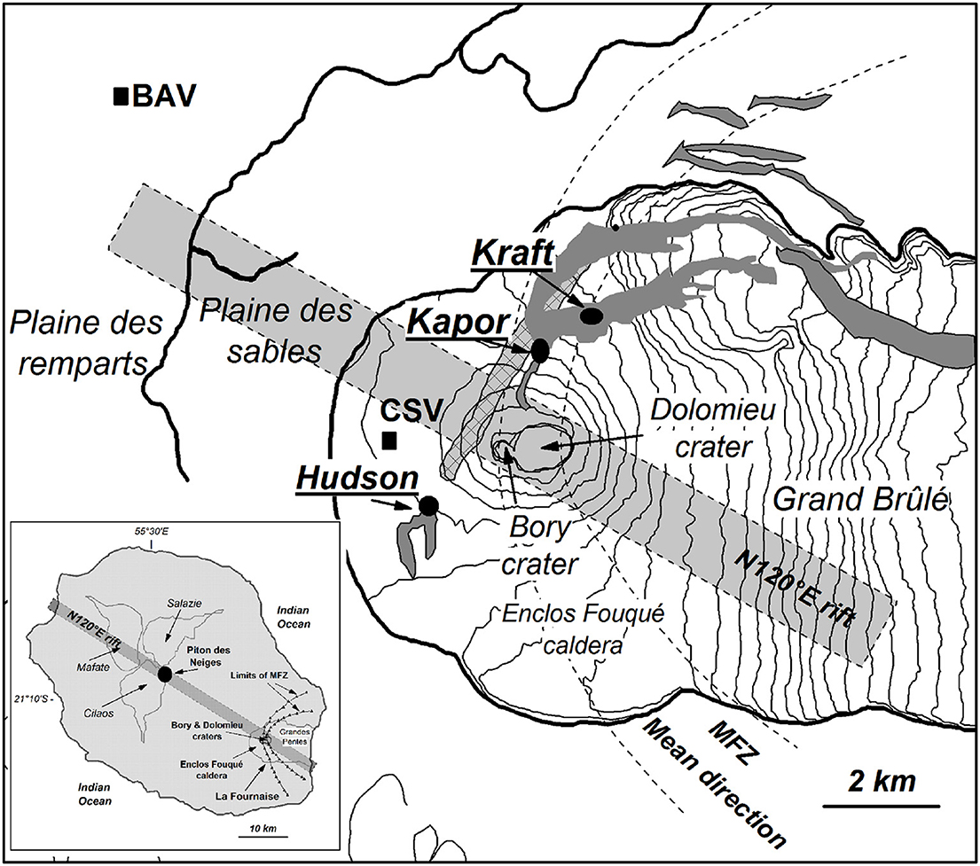
Figure 1. Sketch of La Fournaise volcano, from Wawrzyniak et al. (2017). BAV and CSV are the electromagnetic stations. Lava flows emitted by Krafft, Kapor, and Hudson cones are in dark gray color. Dashed lines represent the main fracture zone along which most fissure eruptions occur. The gray rectangle illustrates the regional N120°E volcanic and fissural axis. Gray cross pattern corresponds to the trace of main earthquakes associated with the March 9, 1998, crisis.

The CSV data are processed using SS configuration, and RR configuration with BAV magnetic data. Sixteen target frequencies (_fk)k are defined ranging from 1.56 to 12.5 mHz. K_per is fixed to 128, and c_overlap is 0.71. This yields a number N_stat of 10,000 data Fourier coefficients for the highest frequency and 1,000 for the lowest. The time bandwidth factor τ (parameter TBW in the code) is 4, and the lower thresholds $T{h}_{B{B}^r}$ and Th_EB are set to 0. The BI regression is controlled by the probability of rejection p_rej, which is 0.05, and the number of BI iterations N_BI is set to 3.

The ME and BI results in SS configuration are shown in Figures 2 and 3, respectively. First, we observe SS apparent resistivity relative difference and phase difference between BIRRP and Razorback. The ME apparent resistivity differs by less than 10% on the xy, yx, and yy components (Figure 2). The phase difference is less than 2°. The relative differences on the xx component are higher, but the absolute value ρ_xx is two orders of magnitude lower than ρ_xy, ρ_yx, and ρ_yy.

FIGURE 2

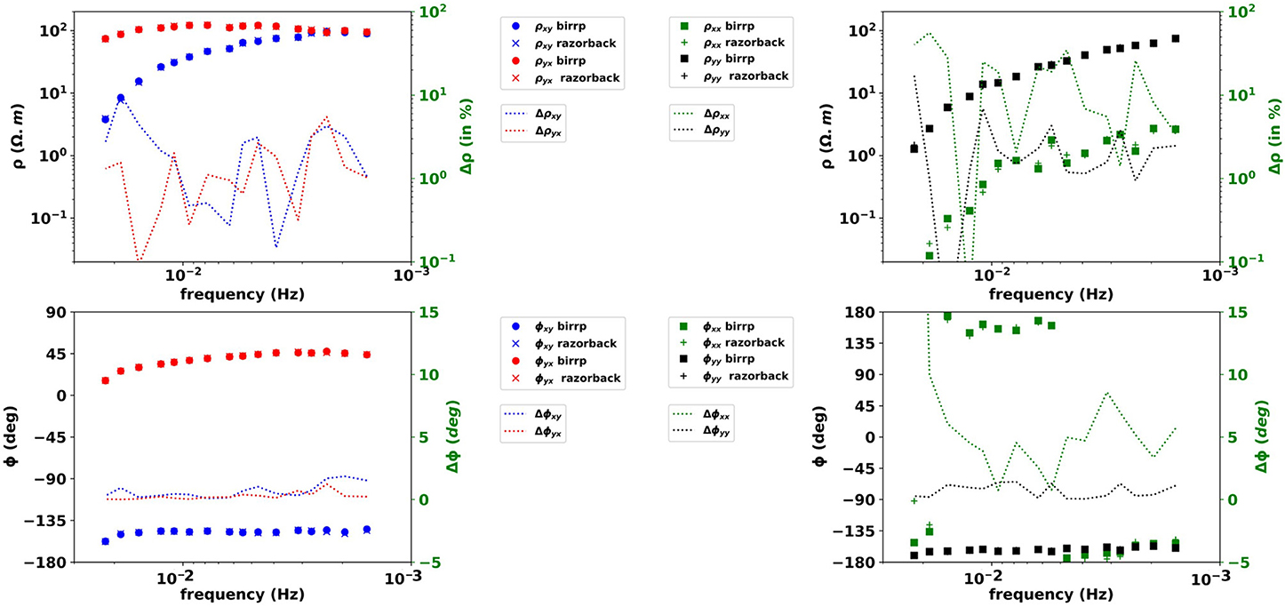
Figure 2. M-estimator results in SS configuration. Upper left: apparent resistivity xy in blue and yx in red from birrp (circles) and razorback (crosses) with scales on the left axis, relative differences between birrp and razorback results (dotted lines) for xy (blue) and yx (red) with scales on the right axis. Lower left: same as upper left but for phase but with absolute differences (dotted lines). Upper Right: apparent resistivity xx in green and yy in black from birrp (squares) and razorback (plus) with scales on the left axis, relative differences between birrp and razorback results (dotted lines) for xx (green) and yy (black) with scales on the right axis. Lower Right: same as upper left but for phase but with absolute differences (dotted lines).

FIGURE 3

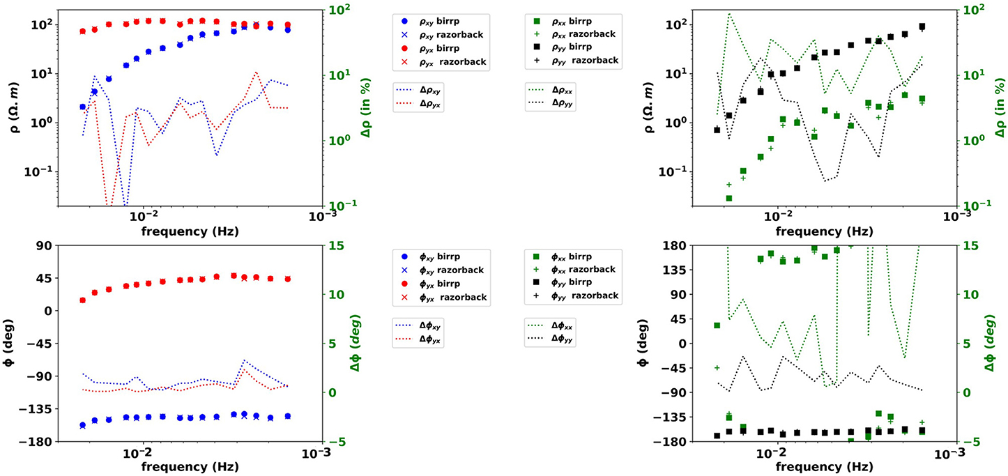
Figure 3. Bounded Influence results in SS configuration. Same legend as Figure 2 but for BI results.

The BI apparent resistivity differs from less than 12% on the xy and yx components to less than 20 % on the yy component (Figure 3). The phase difference is less than 3° on xy and yx and 4° on yy. Although the principle is the same, our implementation of the bounded influence algorithm differs in the computation of leverage weights from the hat matrix and in the definition of the increment of intermediate steps of the BI algorithm.

The two-stage RR ME (Figure 4) shows the apparent resistivity relative difference reaching 20 % on the xy component, less than 3 % on the yx component and less than 30 % on yy. The xy and yy components involve the H_y local and remote magnetic fields. The remote magnetic field component H_y has been diagnosed as biased in Wawrzyniak et al. (2017).

FIGURE 4

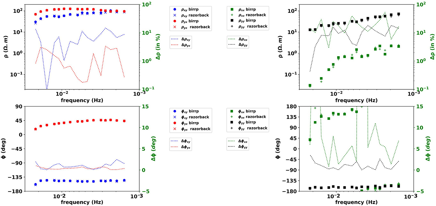
Figure 4. M-estimator results in RR configuration. Same legend as Figure 2 but for RR results.

Thus, the impact of introducing a noisy RR station in the two-stage RR method leads to a moderate discrepancy between the BIRRP and Razorback estimates.

The two-stage RR BI (Figure 5) shows the apparent resistivity relative difference reaching 10 % on the xy and yx component and reaching several tens of percent on xx and yy. Absolute phase difference is still below 3° onxy and yx.

FIGURE 5

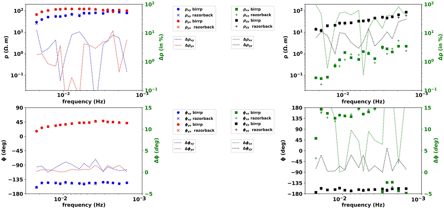
Figure 5. Bounded Influence results in RR configuration. Same legend as Figure 2 but for RR results.

Apart from the data loading [the load_data() function], the impedance estimates presented in Figures 5, 3 for Razorback are obtained with the following code:

5. Advanced Uses

5.1. Testing All Possible Remote Reference Combinations

In the following, we show how the Razorback library allows the user to run one processing method, such as classical M-estimator or bounded influence regression, on a given signal set for any combination of RR stations. We assess the efficiencies of both ME and BI methods on a noisy peri-urban dataset.

Our experimental dataset is a synchronous array of MT stations from a CSEM/MT survey realized in the framework of the European FP7 project IMAGE. The survey area is a 10 by 10 km square located on the western side of the city of Strasbourg (Figure 6). The main geothermal targets in the Upper Rhine Graben are fractured zones within the basement or at the transition zone between the basement and the sedimentary cover. Unfortunately, in such a peri-urban context, the exploration of sedimentary basins using MT is challenging due to the presence of anthropogenic sources (DC railway, factories, power lines and so forth), leading to biased MT soundings.

FIGURE 6

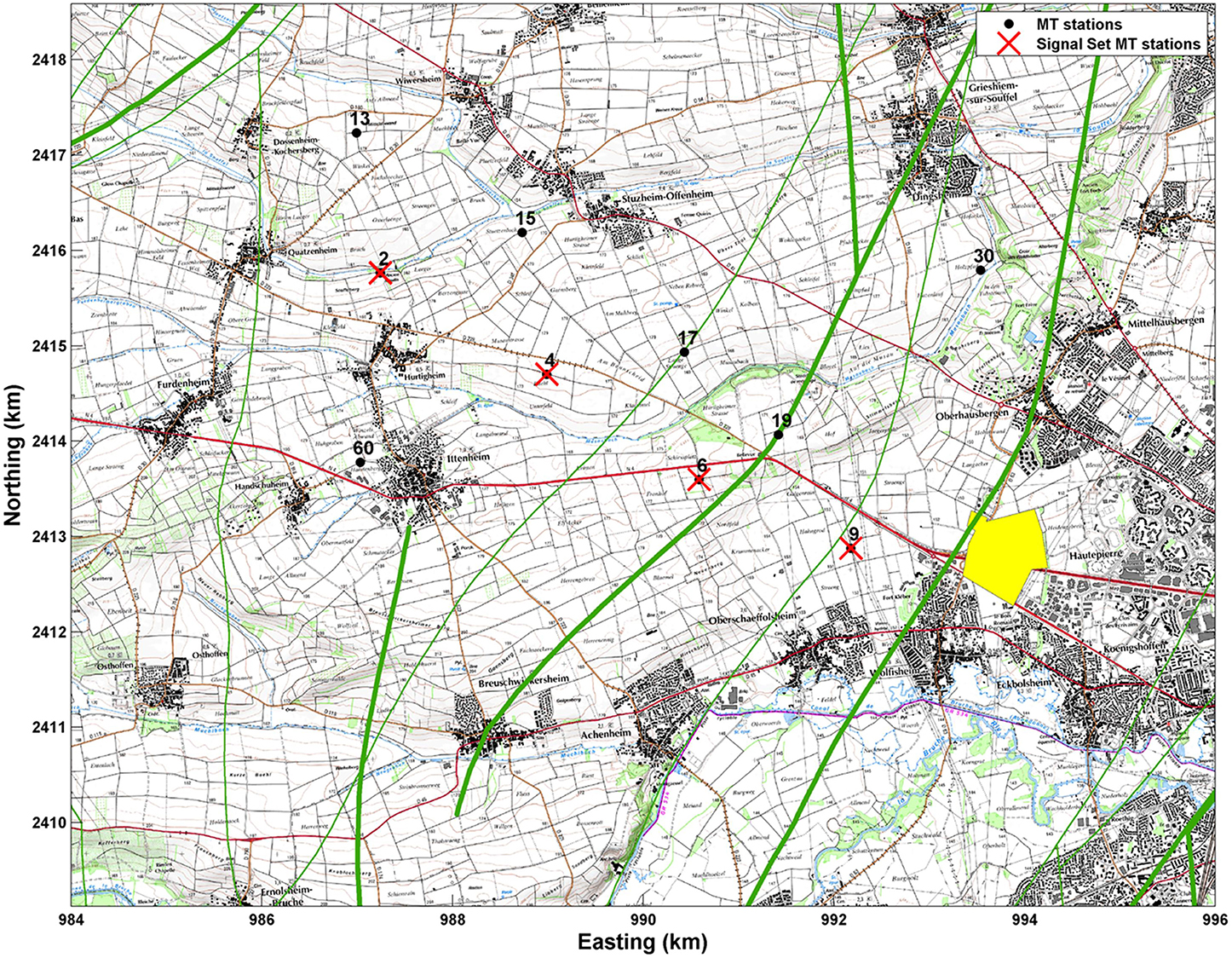
Figure 6. Map of the MT stations deployed on the western side of Strasbourg. Black dots: complete station set. Red crosses: “local” station inserted in the SignalSet object. Green lines: major geological faults. Red line: seismic profile. Yellow area: geothermal plant area.

We use 6 synchronous MT stations (ADU07 acquisition system, Metronix). Four “local” stations are located in the area of interest (stations 2, 4, 6, and 9) and have a 128 Hz sampling rate. Two “distant” remote reference stations are also used: one is installed in Schwabwiller (5 channel MT station, 30 km North), and the other is the Welschbruch geomagnetic observatory (recording horizontal magnetic field only, located at the Welschbruch pass, Le Howald, 30 km South).

We process station 4 using sites 2, 6, and 9 as “local” remote stations and Schwabwiller (RR99) and Welschbruch (RR100) stations as “distant” remote stations. This allows 31 possible combinations of remote stations in addition to the single site processing. We perform two-stage M-estimate (ME) and bounded influence (BI) robust processing without pre-filtering for both the first and second stages. Thirty-two output frequencies, ranging from 1 mHz to 32 Hz, are targeted. At the lowest frequencies, for some combinations of RRs, the computation does not converge. This is due to the weak signal-to-noise ratio and the small amount of Fourier data.

Quality assessment is performed on the MT soundings obtained from combinations of remote channels. First, components of apparent resistivity ${\rho }_{xy,yx}^a$ and impedance phase ϕ_xy,yx are displayed in Figure 7 for ME and BI. ME soundings (Figure 7, upper part) exhibit significant variability in the [20 mHz–1 Hz] band. Some combinations show non-physical resistivity and phase variations (i.e., artifacts up to one order of magnitude on the ρ_yx component and 40° on ϕ_yx). BI soundings (Figure 7, lower part) show less variability in the same frequency band as soon as distant RRs are used. Similar to the ME results, ϕ_yx exhibits a 35° shift, centered on the 0.1 Hz frequency, but with a narrower frequency band imprint. There are more artifacts with wider frequency bands and larger amplitudes in the ME results than in the BI results.

FIGURE 7

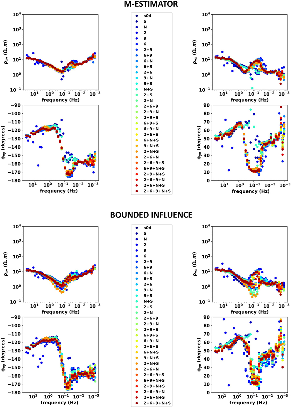
Figure 7. Upper section: M-estimator results. SITE 04 with local RRs 2, 6, and 9 and distant RRs Welschbruch (RR100) and Schwabwiller (R99). No error bars. TF estimates for all possible combinations of RR stations. Apparent resistivity curves ρ_xy (top left) and ρ_yx (top right) and phases ϕ_xy (bottom left) and ϕ_yx (bottom right) are shown in dots, with a color code corresponding to the associated combination of RR stations(the associated legend is displayed on the center). Lower section: bounded Influence results. Same legend as above.

The sounding quality assessment is completed with phase tensor (PT) analysis (Caldwell et al., 2004). Booker (2014) suggests that “smooth variation of the phase tensor with period and position is a strong indicator of data consistency.” Some main features of the PT are the orientation of its principal axis α − β; the length of its principal axis Φ_max; its ellipticity λ that ranges from 0 to 1, and its skew angle β which are indicators of the dimensionality of the data. Low values of ellipticity indicate a 1D medium (Bibby et al., 2005), whereas absolute values of β angles below 10° indicate a 2D medium (Booker, 2014). A 1D medium is characterized by a low λ value and associated with |β| <10°. A 2D medium is characterized by larger values of λ and |β| <10°. A 3D medium is characterized by |β| >10°. Consequently, the normalized phase tensor, i.e., the PT with the longer axis Φ_max normalized to 1, is displayed for all frequencies and RR combinations. Ellipses are filled with a color bar indexed either on their ellipticity value (left panel in Figure 8) or their β angle (right panel, same figure).

FIGURE 8

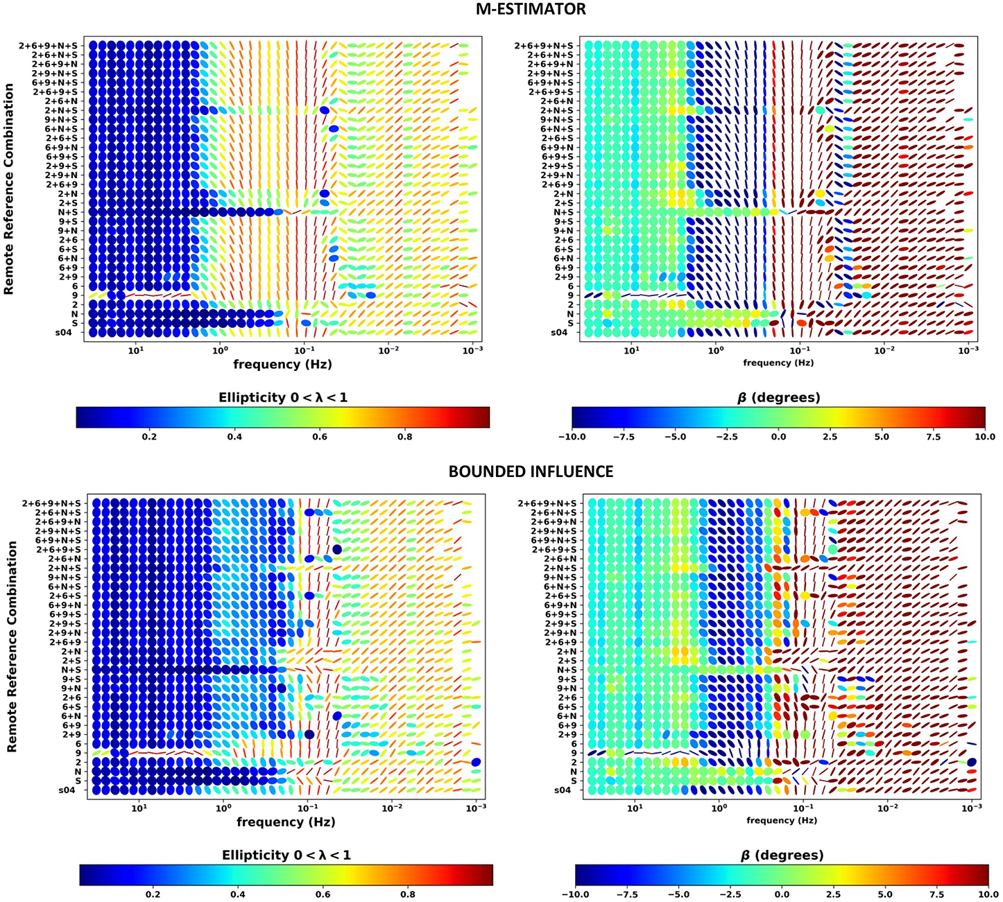
Figure 8. Upper section: M-estimator results. Site 4 with local RRs 2, 6, and 9 and distant RRs Welschbruch (rr100) and Schwabwiller (rr99). Left: normalized phase tensor for all combinations of RR as a function frequency filled with their ellipticity λ value (1D indicator). Right: normalized phase tensors filled with β angle (2D indicator) value; the color bar is limited to [-10° 10°] range. Lower section: bounded influence results. Same legend as above.

Comparing upper and lower part of Figure 8 highlights the superiority of BI processing in the [0.2–2 Hz] band. In this band, the M-estimator leads to high ellipticity values, which would be associated with a 3D medium. In contrast, the BI results indicate a 1D medium with low ellipticity values. In addition, the BI PT curves exhibit smoother frequency variations.

An important observation can be made from the M-estimator results: the combination of a maximum of RR leads to discontinuous PT behavior. Smoother behavior is obtained for combinations of sites 02, 99 and 100. When sites 06 and 09 are added as RRs, discontinuous PTs are observed. This can have a high impact for any MT operator working on a peri-urban context and using ME two-stage processing: introducing additional noisy RR can degrade the sounding quality.

However, ME MT soundings associated with a selection of PT curves (RRs 99, 100, 99+100, 6+99+100, 6+9+99+100, and 2+6+9+99+100) are shown in Figure 9, upper part. The selected results are scattered, and phase and apparent resistivity artifacts still persist in the [0.02–1 Hz] band. Similarly, the BI soundings associated with the same combinations of RRs in Figure 9, lower part. Since 4 remotes are used, the MT soundings are similar. However, both phases ϕ_xy and ϕ_yx show sharp variations in the [0.5–1 Hz] band that can be attributed to persistent noise contamination of the data. Multiple RR two-stage BI processing helps reduce noise contamination of the dataset but cannot eliminate it in this case.

FIGURE 9

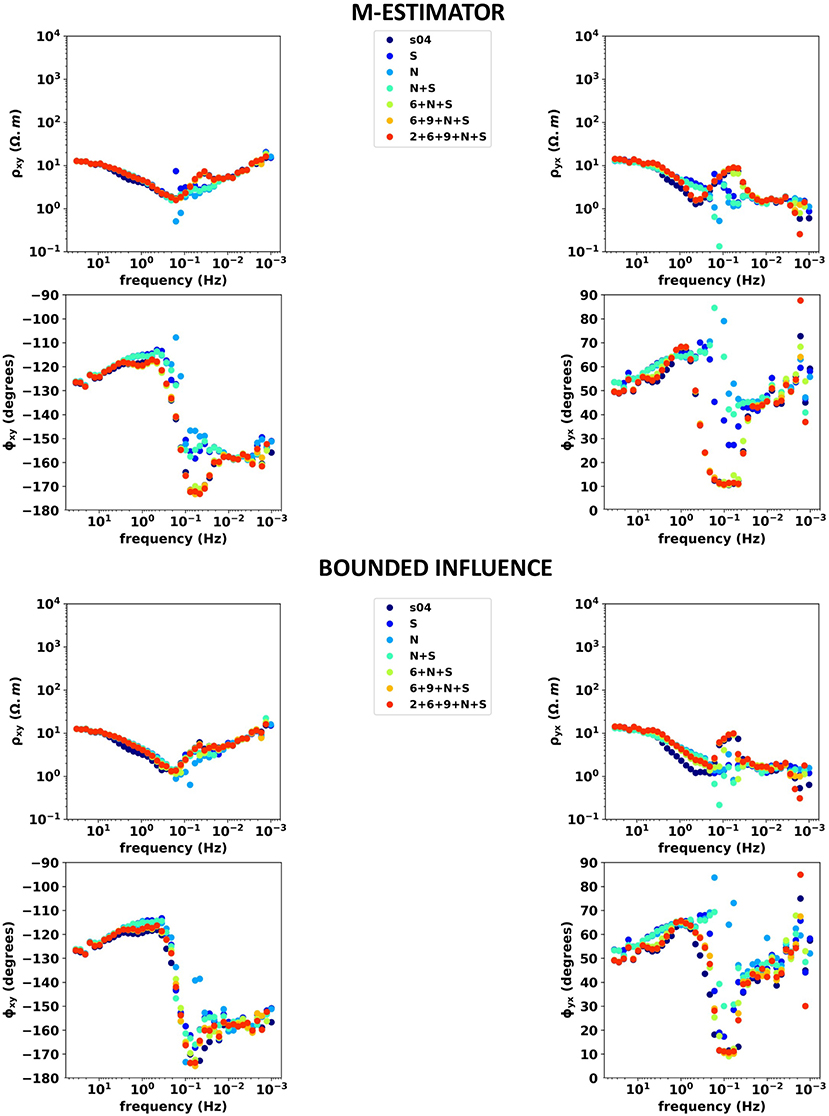
Figure 9. Upper section: selected M-estimator results. SITE 04 with local RRs 2, 6, and 9 and distant RRs Welschbruch (RR100) and Schwabwiller (R99). No error bars. TF estimates for a selection of combinations of RR stations. Apparent resistivity curves ρ_xy (top left) and ρ_yx (top right) and phases ϕ_xy (bottom left) and ϕ_yx (bottom right) are shown in dots, with a color code corresponding to the associated combination of RR stations(the associated legend is displayed on the center). Lower section: selected Bounded Influence results. Same legend as above.

A jupyter notebook dedicated to the robust processing and handling of this data set is provided by the authors and available at https://github.com/BRGM/razorback/blob/doc/docs/source/tutorials/survey-study.ipynb.

5.2. Time-Lapse Magnetotellurics

The library also allows performing continuous time-lapse processing. In Wawrzyniak et al. (2017), time-lapse MT estimates were computed using bounded influence robust processing in both single site and RR configurations in the framework of volcano monitoring. The time resolution between consecutive estimates is of 48 h.

The dataset is the same as in section 4. Horizontal components of the electric and magnetic fields were sampled every 20 s. Continuous time series were available from 1996 to 1999 at CSV and from 1997 to March 20, 1998, at BAV. In March 1998, a major eruption occurred and lasted for 6 months, during which 60 10⁶ m³ of lava was expelled.

RR (not shown here) and single site processing at a period of 80 s show apparent resistivity determinant variations synchronous with the eruption (Figure 10). At CSV, the resistivity shows a continuous two order of magnitude decrease, reaching several local minima until April, and then slowly recovers its pre-eruptive values when the volcanic crisis reduced in activity. BAV shows a short one and a half order of magnitude decrease at the beginning of the eruptive crisis. Further data analyses are provided in Wawrzyniak et al. (2017).

FIGURE 10

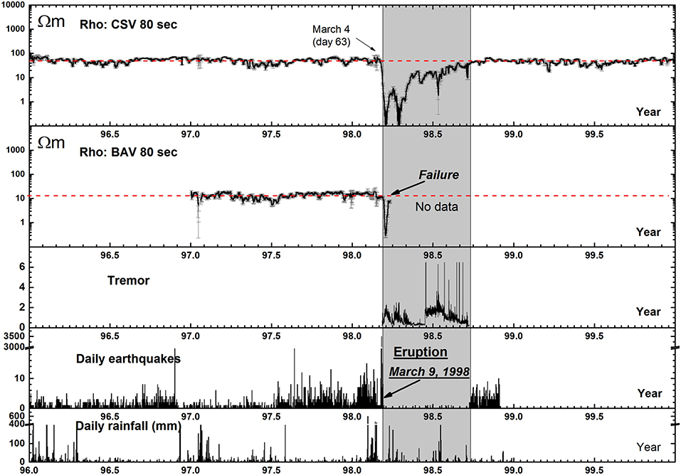
Figure 10. Time-Lapse bounded influence processing, in single site configuration, from Wawrzyniak et al. (2017). From top to bottom: resistivity of the determinant of the impedance tensor values at CSV and BAV for the 80 s period computed by single MT method between 1996 and the end of 1999, tremor activity and daily number of earthquakes, and daily rainfall.

6. Conclusions

This paper shows the advantages of using a modular library for robust processing of MT array data. Razorback is designed to handle and process the large datasets commonly encountered in MT exploration surveys, with minimal memory footprint. After validation of TF estimates by comparison with existing codes, two kinds of study have been performed. First, we explored combinations of RRs for different robust procedures. This results in a large amount of estimates of one TF. The phase tensor analysis is used to compare the quality of the estimates. Moreover, the ability of the different robust methods to reduce the impact of noise on soundings has been investigated. This is of particular interest for geophysicists processing a full MT survey dataset in anthropogenic environment. In addition, continuous time-lapse MT processing has been performed and shows promising results for subsurface monitoring of volcanoes or geothermal reservoirs.

The MT processing workflow mainly consists of (i) data analysis and transformation, (ii) TF estimation, and (iii) quality check of estimated quantities. We propose the open source Razorback library as a collaborative tool to perform these different tasks. For the first step, the library offers elaborated time series manipulations, state of the art DFT computation, and coefficient of determination pre-filtering. Alternate types of pre-filtering exists and can be included. Provided a detection method, the current features can eliminate the identified corrupted time segments. Concerning the second step, a category of standard robust procedures has been implemented. A well-tested set of weighting function sequences is available and can be easily enriched. Alternative categories of TF estimation procedures (e.g., the RMEV approach proposed by Egbert, 1997) could be included and would benefit from the other library features. Regarding the third step, a range of quality check methods exists and could be integrated in the library. Using the modular Razorback library, the MT practitioner fully controls the above workflow.

Data Availability Statement

The Razorback library is available at https://github.com/BRGM/razorback. The data sets analyzed in this article will be made available by the authors, without undue reservation, to any qualified researcher upon reasonable request.

Author Contributions

FS did most of the python language programming. PW designed the MT transfer function tools and validated extensively the library.

Funding

The Razorback library has been developed in the framework of the BRGM-funded projects EDGARR, OPTMT, and Benchmark MT. The MT dataset from Alsace has been acquired and processed in the framework of the IMAGE FP7 project, which has received funding from the European Union's Seventh Program for research, technological development and demonstration under grant agreement No: 608553. Part of the dataset provided as test-data were acquired with instruments of the French national pool of portable magnetotelluric instruments EMMOB (INSU-CNRS) and within activities of the Labex G-Eau-Thermie profonde program. MT data from La Fournaise volcano were used courtesy of Jacques Zlotnicki.

Conflict of Interest

The authors declare that the research was conducted in the absence of any commercial or financial relationships that could be construed as a potential conflict of interest.

Supplementary Material

The Supplementary Material for this article can be found online at: https://www.frontiersin.org/articles/10.3389/feart.2020.00296/full#supplementary-material

References

Bibby, H., Caldwell, T., and Brown, C. (2005). Determinable and non-determinable parameters of galvanic distortion in magnetotellurics. Geophys. J. Int. 163, 915–930. doi: 10.1111/j.1365-246X.2005.02779.x

CrossRef Full Text | Google Scholar

Booker, J. R. (2014). The magnetotelluric phase tensor: a critical review. Surv. Geophys. 35, 7–40. doi: 10.1007/s10712-013-9234-2

CrossRef Full Text | Google Scholar

Cagniard, L. (1953). Basic theory of the magneto-telluric method of geophysical prospecting. Geophysics 18, 605–635. doi: 10.1190/1.1437915

CrossRef Full Text | Google Scholar

Caldwell, T. G., Bibby, H. M., and Brown, C. (2004). The magnetotelluric phase tensor. Geophys. J. Int. 158, 457–469. doi: 10.1111/j.1365-246X.2004.02281.x

CrossRef Full Text | Google Scholar

Carbonari, R., D'Auria, L., Di Maio, R., and Petrillo, Z. (2017). Denoising of magnetotelluric signals by polarization analysis in the discrete wavelet domain. Comput. Geosci. 100, 135–141. doi: 10.1016/j.cageo.2016.12.011

CrossRef Full Text | Google Scholar

Chave, A. D., and Jones, A. G. (2012). The Magnetotelluric Method: Theory and Practice. Cambridge University Press. doi: 10.1017/CBO9781139020138

CrossRef Full Text | Google Scholar

Chave, A. D., and Thomson, D. J. (1989). Some comments on magnetotelluric response function estimation. J. Geophys. Res. Solid Earth 94, 14215–14225. doi: 10.1029/JB094iB10p14215

CrossRef Full Text | Google Scholar

Chave, A. D., and Thomson, D. J. (2003). A bounded influence regression estimator based on the statistics of the hat matrix. J. R. Stat. Soc. Ser. C Appl. Stat. 52, 307–322. doi: 10.1111/1467-9876.00406

CrossRef Full Text | Google Scholar

Chave, A. D., and Thomson, D. J. (2004). Bounded influence magnetotelluric response function estimation. Geophys. J. Int. 157, 988–1006. doi: 10.1111/j.1365-246X.2004.02203.x

CrossRef Full Text | Google Scholar

Chave, A. D., Thomson, D. J., and Ander, M. E. (1987). On the robust estimation of power spectra, coherences, and transfer functions. J. Geophys. Res. Solid Earth 92, 633–648. doi: 10.1029/JB092iB01p00633

CrossRef Full Text | Google Scholar

Dask Development Team (2016). Dask: Library for Dynamic Task Scheduling.

Di Giuseppe, M. G., Troiano, A., and Patella, D. (2018). Separation of plain wave and near field contributions in magnetotelluric time series: a useful criterion emerged during the Campi Flegrei (Italy) prospecting. J. Appl. Geophys. 156, 55–66. doi: 10.1016/j.jappgeo.2017.03.019

CrossRef Full Text | Google Scholar

Egbert, G. D. (1997). Robust multiple-station magnetotelluric data processing. Geophys. J. Int. 130, 475–496. doi: 10.1111/j.1365-246X.1997.tb05663.x

CrossRef Full Text | Google Scholar

Egbert, G. D., and Booker, J. R. (1986). Robust estimation of geomagnetic transfer functions. Geophys. J. Int. 87, 173–194. doi: 10.1111/j.1365-246X.1986.tb04552.x

CrossRef Full Text | Google Scholar

Escalas, M., Queralt, P., Ledo, J., and Marcuello, A. (2013). Polarisation analysis of magnetotelluric time series using a wavelet-based scheme: a method for detection and characterisation of cultural noise sources. Phys. Earth Planet. Interiors 218, 31–50. doi: 10.1016/j.pepi.2013.02.006

CrossRef Full Text | Google Scholar

Gamble, T. D., Goubau, W. M., and Clarke, J. (1979). Magnetotellurics with a remote magnetic reference. Geophysics 44, 53–68. doi: 10.1190/1.1440923

CrossRef Full Text | Google Scholar

Goubau, W. M., Gamble, T. D., and Clarke, J. (1978). Magnetotelluric data analysis: removal of bias. Geophysics 43, 1157–1166. doi: 10.1190/1.1440885

CrossRef Full Text | Google Scholar

Junge, A. (1996). Characterization of and correction for cultural noise. Surv. Geophys. 17, 361–391. doi: 10.1007/BF01901639

CrossRef Full Text | Google Scholar

Kirkby, A., Zhang, F., Peacock, J., Hassan, R., and Duan, J. (2019). The MTPY software package for magnetotelluric data analysis and visualisation. J. Open Sour. Softw. 4:1358. doi: 10.21105/joss.01358

CrossRef Full Text | Google Scholar

Krieger, L., and Peacock, J. R. (2014). MTPY: a python toolbox for magnetotellurics. Comput. Geosci. 72, 167–175. doi: 10.1016/j.cageo.2014.07.013

CrossRef Full Text | Google Scholar

Larnier, H., Sailhac, P., and Chambodut, A. (2016). New application of wavelets in magnetotelluric data processing: reducing impedance bias. Earth Planets Space 68:70. doi: 10.1186/s40623-016-0446-9

CrossRef Full Text | Google Scholar

Sims, W., Bostick Jr, F., and Smith, H. (1971). The estimation of magnetotelluric impedance tensor elements from measured data. Geophysics 36, 938–942. doi: 10.1190/1.1440225

CrossRef Full Text | Google Scholar

Streich, R., Becken, M., and Ritter, O. (2013). Robust processing of noisy land-based controlled-source electromagnetic data. Geophysics 78, E237-E247. doi: 10.1190/geo2013-0026.1

CrossRef Full Text | Google Scholar

Szarka, L. (1988). Geophysical aspects of man-made electromagnetic noise in the Earth-a review. Surv. Geophys. 9, 287–318. doi: 10.1007/BF01901627

CrossRef Full Text | Google Scholar

Tikhonov, A. (1950). On determining electric characteristics of the deep layers of the Earth's crust. Dolk. Acad. Nauk. SSSR 73, 295–297.

Google Scholar

Trad, D. O., and Travassos, J. M. (2000). Wavelet filtering of magnetotelluric data. Geophysics 65, 482–491. doi: 10.1190/1.1444742

CrossRef Full Text | Google Scholar

Vozoff, K. (1972). The magnetotelluric method in the exploration of sedimentary basins. Geophysics 37, 98–141. doi: 10.1190/1.1440255

CrossRef Full Text | Google Scholar

Ward, S. H. (1967). “Part A. Electromagnetic theory for geophysical applications,” in Mining Geophysics, Volume II, Theory (Society of Exploration Geophysicists), 13–196. doi: 10.1190/1.9781560802716.ch2a

CrossRef Full Text | Google Scholar

Wawrzyniak, P., Zlotnicki, J., Sailhac, P., and Marquis, G. (2017). Resistivity variations related to the large March 9, 1998 eruption at la Fournaise volcano inferred by continuous MT monitoring. J. Volcanol. Geotherm. Res. 347, 185–206. doi: 10.1016/j.jvolgeores.2017.09.011

CrossRef Full Text | Google Scholar

Zhang, Y., and Paulson, K. (1997). Enhancement of signal-to-noise ratio in natural-source transient magnetotelluric data with wavelet transform. Pure Appl. Geophys. 149, 405–419. doi: 10.1007/s000240050033

CrossRef Full Text | Google Scholar