 Tamaz Chelidze
 Giorgi Melikadze
 Tengiz Kiria
 Tamar Jimsheladze
- M. Nodia Institute of Geophysics, Tbilisi, Georgia
In 20th century, more than 10 strong earthquakes (EQs) of magnitudes 6,7 hit South Caucasus, causing thousands of casualties and gross economic losses. Thus, strong-EQ forecast is an actual problem for the region. In this direction, we developed a physical percolation model of fracture, which considers the final failure of solid as a termination of the prolonged process of destruction: generation and clustering of micro-cracks, till appearance—at some critical concentration—of the infinite cluster, marking the final failure. Percolation provides a model of preparation of an individual strong event (slip or EQ). The natural seismic process contains many such events: the appropriate model is a non-linear stick-slip model, which is a particular case of the general theory of the integrate-and-fire process. Non-linearity of the seismic process is in contradiction with a memoryless Poissonian approach to seismic hazard. The complexity theory offers a chance to improve strong EQs’ forecast using analysis of hidden (non-linear) patterns in seismic time series, such as attractors in the phase space plot. For a regional forecast, we applied the Bayesian approach to assess the conditional probability expected in the next 5 years of strong EQs of magnitudes five and more. Later on, in addition to Bayesian probability assessment, we applied to seismic time series the pattern recognition technique, based on the assessment of the empirical risk function [generalized portrait (GP) method]: nowadays, this approach is known as the support vector machine (SVM) technique. The preliminary analysis shows that application of the GP technique allows predicting retrospectively 80% of M5 events in Caucasus. Besides long- and middle-term forecast studies, intensive work is under way on the short-term (next-day) EQ prediction also. Here, we present the results of multiparametrical (hydrodynamic and magnetic) monitoring carried out on the territory of Georgia. In order to assess the reliability of the precursors, we used the machine learning approach, namely, the algorithm of deep learning ADAM, which optimizes target function by a combination of optimization algorithm designed for neural networks and a method of stochastic gradient descent with momentum. Finally, we used the method of receiver operating characteristics (ROC) to assess the forecast quality of this binary classifier system. We show that the true positive rate statistical measure is preferable for the EQ forecast.
Introduction
Caucasus is located in the central section of the Alpine-Himalayan belt, namely, at the junction of its European and Asian branches. The seismicity of the region is connected with the ongoing northward convergence of the Arabian and Eurasian plates, which began in post-Oligocene (Adamia et al., 2017): now the GPS velocities in South Caucasus with respect to Eurasia vary from 2–5 mm/year in the western part to 12–14 mm/year in the eastern part of the region (Reilinger et al., 2006). Due to this convergence, in the 20th century alone, more than 10 strong earthquakes (EQs) of magnitudes from 6 to 7 hit South Caucasus, causing thousands of casualties and gross economic losses. Thus, the problem of forecast/prediction of strong EQs is important for the region. The following solution to this problem seems to be rational: (i) developing appropriate theoretical models for fracture process of solids and their testing in numerical experiments; (ii) statistical/non-linear analysis of seismic catalogs/geophysical data aiming to forecast long- and middle-term periods of increased probability of strong (say M ≥ 5) EQs, and lastly, (iii) operative forecast (short-time prediction) of the next impending strong event by monitoring geophysical fields, sensitive to tectonic strain variation (hydrodynamic and magnetic fields’ variations).
The EQ forecast/prediction-oriented geophysical network in Georgia consists of seismic stations’ network (from 1890), the network of water-level (WL) monitoring boreholes (from 1988), and the Tbilisi/Dusheti geomagnetic station (from 1840), which has operated systematically for a long time. The summary of results, obtained in Georgia in the framework of the Soviet Union program for EQ prediction, were published by Chelidze et al. (1995).
Theoretical Models
The general approach to developing a physical model of seismic activity can be divided into two main problems: (i) constructing the physical model of the sequence of events preceding the main rupture (a single strong EQ) and (ii) analyzing the complexity of the entire seismic catalog, considered as time series of EQs (following the stick-slip or integrate-and-fire model).
Physical Model of a Single Strong Event Preparation
In series of papers (Chelidze, 1986, 1987; Chelidze and Kolesnikov, 1984), we developed the physical model of the fracture process based on percolation theory (Sahimi, 1994; Stauffer and Aharony, 1994; Aharony and Stauffer, 2010; Saberi, 2015), which considers the final failure as a termination of the prolonged process of damage accumulation in disordered media (Charmet et al., 1990; Herrmann and Roux, 1990). The model considers the fracture process as generation/coalescence of elementary fractures (with increasing volumetric concentration x) and their clustering, till appearance, at some critical concentration xc, of the infinite cluster (IC) of cracks (the major rupture), marking the final destruction of the material. For the random distribution of elementary cracks with a constant interaction length L, both percolation theory and laboratory experiments (Zhurkov et al., 1977) prove that transition from a diffuse fracture state to the appearance of the IC (main rupture) occurs at a critical value of damage N:
where N is the number of elementary cracks in the unit volume, ke is the proportionality constant, and L is the mean size of cracks. According to Chelidze (1987), the value of ke varies in the range 2.5–7 with the mean value 4 and is quite stable for very different values of N–1/3 and L (Zhurkov et al., 1977). Percolation fracture theory provides also a mathematical model of preparation of a single large-scale strong dynamic event (slip or EQ).
It is clear that generation and merging of elementary cracks are connected with the emission of energy due to redistribution of local stresses. The appearance of each new crack provokes seismic energy emission with effective amplitude, depending on the increment of the size of the existing clusters after addition of a new elementary crack (Chelidze and Kolesnikov, 1984). The emitted energy or conditional amplitude A of the event, generated by the appearance of a new elementary crack, is
where A0 is a conventional amplitude of the dynamic signal, due to nucleation of a (isolated) single defect, k is the number of clusters merged by addition of an elementary defect, and si is the number of sites in the ith cluster, formed by merging two clusters. Thus, the value of A depends on the increment of the size of the resulting cluster formed by the coalescence of cracks caused by the appearance of a new elementary crack.
The percolation model allows formulating several possible precursors of the main fracture (Chelidze, 1986, 1987), for example, some anomalies in the behavior of the so-called percolation functions at approaching the final fracture, such as (i) increased divergence of finite size of clusters s, in other words, a strong increase in the scatter of amplitude A at approaching the critical crack concentration xc; (ii) a strong increase of the number of large pulses, and (iii) a decrease of the slope of magnitude–frequency relation. Many of these precursors of impending final failure are observed in laboratory acoustic emission as well as in seismic time series (STS) preceding strong EQ (Chelidze, 1986, 1987).
At the same time, it is clear that such a separate event—formation of a single major rupture—is only an isolated episode of the long-term seismic process, containing many strong events (EQs). Analysis of this process calls for development of different models, which consider the mechanism of generation of a continuous sequence of separate strong events.
Modeling the Pattern of a Seismic Process—Long Time Series of EQs
We know that a seismic process is a large-scale continuous stick-slip motion along the fault plane, generating a sequence of dynamic events of different magnitudes: the approach was initiated in other works (Brace and Byerlee, 1966; Burridge and Knopoff, 1967; Ruina, 1983). Such a stick-slip motion is a particular case of the general theory of the non-linear integrate-and-fire process (Pikovsky et al., 2003). On the laboratory slider-spring model, we show that a weak regular forcing synchronized stick-slip with this impact, which confirms the complex (non-linear) nature of the seismic process (Chelidze et al., 2005; 2006, 2010; Chelidze and Lursmanashvili, 2003; Chelidze and Matcharashvili, 2013, 2015). Non-linear models of the seismic process founded on complexity theory are in contradiction with a memory-less purely Poissonian approach to seismic hazard assessment (SHA), where all EQs are considered as independent events (Cornell, 1968; McGuire, 1976; Bender and Perkins, 1987; Ogata, 1998).
In the next section, we show that the complexity theory offers a chance to improve methods of strong EQs’ forecast using analysis of hidden (non-linear) patterns in STS, such as attractors in the phase space (PS) plot.
Long-Term and Middle-Term EQ Forecast [Bayesian Approach, Support Vector Machines (SVMs), and Phase Space Portraits (PSPs)]
Bayesian Approach
Besides the standard SHA of Georgia, in 1990, the Georgian Institute of Geophysics carried out together with the Russian Institute of Physics of Earth pioneering investigations related to developing the Bayesian mathematical model of EQ forecast by analysis of i precursors (Sobolev et al., 1991), which was called the map of expected earthquakes (MEEQ). We used Bayes equation for assessing conditional probabilities of EQ occurrence P(D1| K) in a given spatial pixel:
where D1 and D2 are correspondingly alarm and quiescence diagnoses, Ki is the ith precursor, P(K1| D1) and P(Ki| D2) are correspondingly probabilities of successful prediction and false alarm using n predictors, P(D1) is the unconditional stationary probability of the occurrence of an EQ of M ≥ 5 in a spatial cell examined, and P(D2) = 1 - P(D1) is the unconditional stationary probability of the occurrence of an EQ of M ≥ 5.
The compilation of MEEQ envisions three steps: (i) generation of the map of stationary conditional probability Pscp(D1) of a strong EQ of M ≥ 5 in the region (Caucasus) for a full catalog; (ii) compilation of non-stationary conditional probability P(D1| K) of the occurrence of a strong EQ of M ≥ 5 using the ensemble of several predictors for a given time interval; (iii) compilation of probability gain (effectivity), obtained by using previously mentioned predictive signs in the time and space domains.
The basis of calculations was the seismic catalog of Caucasus from 1962 to 1987 (Sobolev et al., 1991), which is considered as homogeneous (events of M2.5 were registered without omission). Unfortunately, the regional catalog after 1987 due to political turmoil is of less quality.
The map of stationary conditional probability Pscp(D1| K) was calculated in the following manner: each strong EQ was represented by its preparatory area Sp, where, according to existing models of focal processes, significant anomalies of geophysical fields are expected—namely, the preparation areas with a size that is an order of magnitude larger than the rupture size L of a given EQ. The area Sp of such a focal zone for an EQ of M ≥ 5 was accepted as a circular area of radius R = 10L, where L ≈ 8 km. Accordingly, the Sp of a single event Sp = πR2 = 5,400 km2. The unconditional stationary probability Pusp(D1) of the occurrence of an EQ of M ≥ 5 in a given spatial cell (pixel) per year is calculated by averaging the data of 36 strong EQs occurring in the period 1962–1983, with clusters taken as a single event. The Pusp(D1) per 5 years per pixel turns out to be 0.09. The stationary conditional probability Pscp(D1| K) was calculated by the Bayes formula, using the stationary predictors—amplitudes of vertical displacements and existence of fault intersections in a given cell.
For the calculation of the non-stationary conditional probability P(D1| K) map, we used the following time series of (time-dependent) predictors in a given pixel: density of seismogenic faults ks, slope of the magnitude–frequency relation γ, seismic activity rate γ (number of events N per unit time), emitted seismic energy Eem. Note that the value of seismogenic faults’ density ks was defined as a function of seismic energy, emitted jointly by faults and activated in the volume V in the time interval Δt. Predictors are calculated as deviations of their current values from the long-term (background) values, normalized to the mean square error of the averaged background value. The details of calculations of the magnitudes of predictors and their critical values, when the alarm period should be announced, are presented in the literature (Sobolev et al., 1991; Chelidze et al., 1995; Zavjalov, 2006).
We applied the Bayesian approach to assess conditional probability expected in the next 5 years of strong EQ of magnitudes five and larger. Specifically, the probability of alarm was calculated by the above Bayes equation, where P(D1| K) was considered as a time-variable probability. The probabilities of successful forecasts and false alarms as well as the mean alarm periods were estimated from the retrospective analysis of predictors’ database and the regional catalog of strong EQs. The forecast was recognized as a successful one if the EQ preparation area, defined as the circle of radius R = 10L, where L is the half length of the EQ rupture, covers more than half of the pixel with a high value of conditional probability P(D1| K), namely, where the ratio of P(D1| K) to the stationary conditional probability Pscp(D1| K) is of the order of 2 or more. The 5 years’ duration of the alarm period was adopted.
The efficiency or probability gain in the time and space domains (correspondingly Jt and Js), obtained by application of abovementioned methodology, was calculated as
where Npr is the total number of predicted EQs and Nsum is the total number of EQs during summary observation period Ts; Tsa is the summary duration of alarms.
where Ssa is the summary area of alarms and Sobs is the summary area of observations.
The MEEQ compiled for the period 1988–1992 marks an anomaly in the epicentral areas of the Spitak (M6.9, December 1988) and Racha (M7, April 1991) EQs. The Spitak anomaly appears in the MEEQ alarm period beginning from 1986 to 1990. There was no anomaly in MEEQs of the Racha region till 1988, when a stable anomaly appears close to the epicentral area of impending EQ (Sobolev et al., 1991; Chelidze et al., 1995).
The foregoing methodology was further developed and applied to different seismo-active regions of the globe: Central Asia, South California, China, Western Turkey, and Greece (Zavjalov, 2006). In most cases, the probability gain Jt was 2.5 compared to random guess, and the mean area of alarm Ssa occupies only 30% of the total area Sobs with a seismic rate of one EQ per year.
Generalized Portrait (GP)—SVMs
Later on, Chelidze et al. (1995) used for a long-term forecast the pattern recognition technique (GP method), based on the assessment of the empirical risk function (Vapnik and Chervonenkis, 1974; Vapnik, 1984), in addition to Bayesian probability assessment. Nowadays, this approach is known as the SVM technique (Burges, 1998; Nello and Shawe-Taylor, 2000; Steinwart and Christmann, 2008; Theodoridis and Koutroumbas, 2009). The main point of the SVM technique is calculating the so-called Vapnik–Chervonenkis (VC) dimension. The VC measure divides the vector space (where the components of vectors are different EQ predictors) into two classes: EQ alarm and quietness. It is important that the method is not very demanding to the size of the data sample.
The GP technique can be briefly summed as follows: there is a sequence of situations which reflect the existence of some distribution density function P(x). Variable x is a vector, which can have many components (features, symptoms, and predictors). These situations, represented by the corresponding set of predictors, can be linked to a definite class of events ω by some teaching algorithms in assumption that there exists the conditional probability P(ω| x). If ω = 0, then vector x is attributed to the first class, and if ω ≠ 0, the situation belongs to the second class. Both P(x) and P(ω| x) are unknown a priori: all that we know is that they really exist and that these probabilities reveal themselves in the (x, ω) pairs, obtained after n observations of the vector x and corresponding classifications ω: x1, ω1; x2, ω2; x3, ω3 … xn, ωn. From this correspondence set, one should derive a diagnostic rule, which guarantees the minimal number of errors in the used class a of a decision function. The quality F of the rule, which links ω and x as ω = F(x, a), is controlled by the risk function I(F):
where the term q(z) = [ω - F(x, a)]2 is called the risk function. Each classification error increases the function I(F), as in this case, the observed class and the predicted class do not coincide, which means that z ≠ 0 and correspondingly q(z) = 1; on the contrary, if z = 0, i.e., the predicted class is correct, then q(z) = 0 and the risk function I(F) does not increase. Thus, the pattern recognition problem is solved if a chosen risk function is optimal and the risk function I(F) is minimal for a given P(x| ω). The diagnostic rule optimization rests on the analysis of the following features: (i) number of errors, (ii) complexity of rule, and (iii) length of the x, ω-sequence. The practical rule for the application of the GP method is that the dimensionality of the space of predictors d should be at least three times less than the length of the experimental x, ω-sequence l: (l/d) > 3. After this, we search for the simplest class of F-functions, which allows us to construct the optimal hyperplane, dividing the set of x-vectors into two classes. The term GP is attributed to the vector Q, which is normal to the dividing hyperplane. If perfect separation of classes is impossible, the most “naughty” x, ω-pair, which prevents division of classes, is to be excluded, then the next one, and so on, until the two classes are divided without overlapping by the distance R, which represents the width of the dividing strip between two classes. The ratio of the number of withdrawn vectors to the total number of vectors defines the level of diagnostic rule reliability.
The above methodology was applied to forecast periods of strong EQ of M ≥ 5 in Caucasus. The catalog contained 53 events, occurring after 1971. The predictors used earlier in the Bayesian approach, namely, the density of seismogenic faults ks, the slope of the magnitude–frequency relation γ, the seismic activity rate γ (number of events N per unit time), and the emitted seismic energy Eem, were used in the GP approach also. Actually, only 30 active periods before strong EQs were used as the experimental sequence, because considerable time is needed for the accumulation of averaged values of predictors. Most of the training procedures follow a scheme: 24 quarterly values of each predictive function during 6 years, preceding a strong EQ, were picked out. The first 12 values of these sub-predictors were attributed to the second class (quiet period) and the last 12 values to the first class (alarm periods); different schemes were also tested (Chelidze et al., 1995). The retrospective forecast was considered as a successful one if the last 12 quarterly values of the sub-predictor set were recognized as first-class objects. Table 1 represents the results of the application of the GP technique to forecasting the periods of increased EQ hazard level in Caucasus.

Table 1. Results of the application of the GP technique to forecasting the periods of increased EQ hazard level in caucasus using predictor γ or predictors γ and Eem jointly; n is the number of a given class situation—alarm or quietness.
The preliminary analysis shows that application of the GP technique with a predictor γ (the slope of magnitude–frequency relation) allows retrospectively forecasting 85% of periods with M5 events and 100% of calm periods without strong events in Caucasus (Chelidze et al., 1995; Zavjalov, 2006). Addition of a less informative predictor Eem (emitted seismic energy) spoils the total forecast quality by 11%.
Middle-Term Forecast: PSPs
To obtain a middle-term forecast, we analyzed the number of seismic events in a sequential time window—a seismic rate (Sobolev, 2011). The seismic rate is widely used as a proxy of the strain rate in the Earth crust (Dieterich et al., 2000). We performed PS analysis of data sets obtained from the seismic catalog of Caucasus 1960–2011 (Chelidze et al., 2018). The representative magnitude for the period is M2. In this instrumental period, the two largest EQs, Spitak and Racha (M6.9–7), struck the region in 1988 and 1991 correspondingly. Three areas were selected: (i) Batumi area, in order to show the pattern of STS in a seismically (relatively) quiet region; (ii) Spitak; and (iii) Racha. We analyzed both original and declustered, by Riesenberg algorithm (Reasenberg and Matthews, 1988), STS using the catalog of Georgia (Tsereteli et al., 2016). The following parameters of STS were varied: (i) different epicentral areas, where STS were obtained; (ii) length of the time window for the rate count; (iii) year span (periods in the catalog); (iv) periods before and after strong events; and (iv) different magnitude thresholds (Chelidze et al., 2018). The PSPs were compiled using both original STS and STS smoothed by the Savitzky–Golay (SG) filter. The SG filter has the advantage over, for instance, the moving average filter, as the magnitude of the variations in the seismic rate data, i.e., the value of the local extremes, is preserved (Press et al., 2007). Trajectories on PSP plots are obtained by connecting the consecutive phase states in a clockwise direction, which corresponds to an increase in time. For plotting phase plots, we used either standard MATLAB scripts (seism_port or phase_portrait). Both approaches sometimes produce negative values of phase states, which means that the smoothed lagged values in a given window are smaller than in the previous ones. In the following, we only show results, compiled in the following way (Sobolev, 2011): on the X-axis are plotted the mean values of the number N of EQs per n days, and on the Y-axis is plotted a differential of N for the next 10 days, i.e., (Ni=10 – Ni) = dN. The trajectories on PSP plots form a “noisy attractor” with a diffuse source area. Such attractors are common in biological systems (Molaie et al., 2013).
The PS plot analysis reveals some fine details of the seismic process dynamics related to strong EQ precursory/post-event patterns. The plots generally manifest two main features: a diffuse but still limited “source/basin” area, formed by background seismicity, and anomalous orbit-like deviations from the source area, which are related to foreshock and aftershock activity of strong EQs or to appearance of clusters.
In Figure 1, we present an example of application of the PS reconstruction method to EQ time series, which revealed non-linear structures in the PSP for the circular area with radius R = 200 km of the strong Racha EQ (M7), which occurred in West Georgia at 9:12 UTC on 29 April 1991. The used catalog covers the time long before, during, and after the EQ occurrence. The dates on different trajectories mark strong EQ occurrences in the area. The most extended orbits reach the maximal deviations at lags dN equal to 10 or 20 days on the following dates: (i) 1976, August—during swarm of EQs within R = 200 km; (ii) 1991, May—close to the moment of the Racha EQ mainshock, M7.0; (iii) 1991, June—the moment of a strong Java aftershock of the Racha EQ (15 June 1991, M6.2); and (iv) 2009, October—the time of the Racha EQ on 8 September 2009, M6.0 (the late aftershock of the main 1991 Racha EQ).
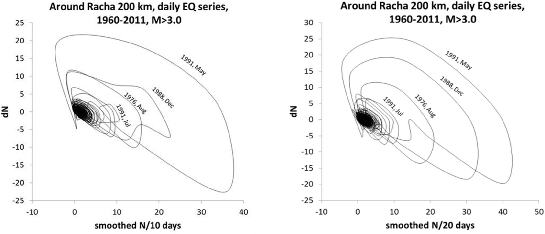
Figure 1. Phase space portraits plotted for the number of EQs N smoothed by the Savitzky–Golay filter versus dN using the declustered catalog (10 and 20 days of smoothed EQ number with a 1-day step) for the area with R = 200 km around the Racha EQ epicenter. On the X-axis are plotted the mean values of the number N of EQs per n days, and on the Y-axis is plotted a differential of N for n days, i.e., (Ni=n - Ni) = dN for n = 10 (left) and 20 (right) days. The dates on trajectories mark strong EQ occurrences.
The whole length of the most extended trajectory with the label 3 May 1991 is 133 days, from start to finish at the source cluster. The time from the moment when a significant deviation from the background seismicity (“noisy” basin) begins to that with the label 3 May 1991 is approximately half of the full orbit duration. We presume that this time is needed to form a “precursory” half orbit, lasting approximately 60 days. We presume that a strong deviation of the orbit from the source area is a precursor of the Racha 1991 event, due probably to foreshock (correlated) activity, not excluded fully by Reasenberg declustering. Indeed, Matcharashvili et al. (2016) showed that after Reasenberg declustering, many correlated events are still left in the catalog.
Similar PSPs were obtained for the Spitak EQ area (Chelidze et al., 2018): the PS orbit begins to deviate from the fuzzy source area approximately 60 days before the Spitak event. It is necessary to note that the long-deviating orbit for 1983 was obtained also in the quiet Batumi area due to the effect of a remote (R ≈ 500 km) 1983 Erzurum EQ (Chelidze et al., 2018). However, in PSPs of Racha and Spitak test areas, there are no orbits connected with the 1983 Erzurum EQ, despite the comparable distance between the EQ and test areas. Probably, this is due to the directivity effect. We conclude that the strong EQ forecast using the PSP approach is promising for revealing deviations in the time domain 30–60 days before the strong event, though the location of impending event remains uncertain.
The results of PSP analysis are intriguing, but we still need many efforts to get definite conclusions: are they just PSPs, or are they real strange attractors obeying the model of deterministic chaos, like those proposed by Sobolev (2011)? The appearance of the strange attractor means that the state of system after some delay repeats itself, i.e., the orbits attain the limit cycle. We cannot expect such regular behavior in a complicated extremely heterogeneous Earth system (see Figure 1), but still deviations of orbits from the source area seem to be informative for EQ source physics.
Short-Term Operational Forecast
Networks, Devices, Data
Besides these statistical models, oriented to regional long- and middle-term forecast studies, intensive work is under way on the short-term EQ forecast/prediction also. The most systematic work in this direction in Georgia is connected with regular monitoring of WL in the network of deep wells, which began in 1988. Here, we present the results of multiparametrical (hydrodynamic and magnetic) monitoring carried out in 2017–2019 on the territory of Georgia.
In this paper, the WL monitoring data in deep wells’ network in Georgia, operated by the M. Nodia Institute of Geophysics (Figure 2), are used. The WL monitoring network in Georgia includes several deep wells, drilled in a confined subartesian aquifer: Kobuleti, Akhalkalaki, Marneuli, Lagodekhi, Ajameti, Chvishi, Nokalakevi, and Oni (Table 1 and Figure 2). The sampling rate at all these wells is 1/min (except Oni, where the sampling rate is 1/10 min). Measurements are done by sensors MPX5010 with a resolution at 1% of the scale (Freescale Semiconductors;1) and recorded by a datalogger XR5 SE-M (Pace Scientific;2) remotely thru a modem, Siemens MC-35i Terminal (Siemens) using program LogXR; the datalogger can acquire WL data for 30 days at the 1/min sampling rate. Variations of WL represent an integrated response of the aquifer to different periodic and quasi-periodic (tidal variation and atmosphere pressure) as well as to non-periodic influences, including generation of EQ-related strains in the Earth crust of the order of 0.1–0.001 microstrain. The atmosphere pressure factors (Figure 3) were subtracted from the summary WL variations.
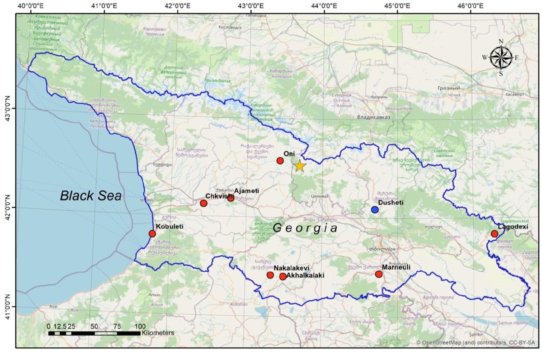
Figure 2. Map of Georgia with location of the deep wells’ network (red circles) for WL monitoring and the Dusheti Geomagnetic Observatory (blue circle). The star marks the location of the 1991 M7 Racha EQ.
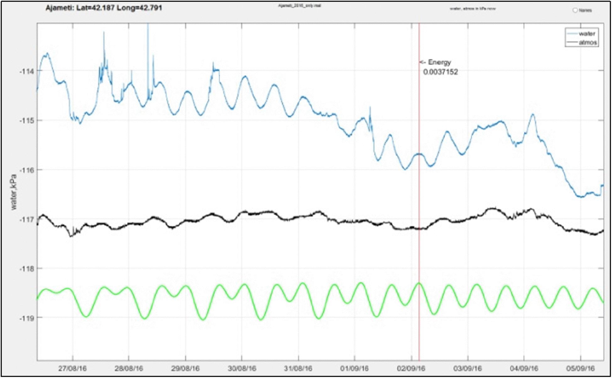
Figure 3. Recording of WL (blue), barometric pressure (black), and computed tidal variations (green) in the Ajameti well before and after the 02/09/2016 Gagra EQ (M4), marked by the red line.
Magnetic variations were recorded at the Dusheti Geophysical Observatory (latitude 42.052N, longitude 44.42E), by the fluxgate magnetometer FGE-95 (Japan), registering x, y, z components at a count rate of 1/s with accuracy of 0.1 nT. The data are representative for a whole territory of Georgia.
Machine Learning (ML) Methodology
Quantitative analysis of impacts of different components of endogenous and exogenous origins in the observed integral dynamics remains one of the main geophysical problems. Especially important, taking into account their possible prognostic value, is identifying the impact of non-periodic processes related to the EQ generation. We investigate the dynamics of regular and non-periodic components in the considered time series using special ML programs: ADAM and ROC (Diederik and Ba, 2014). The advances in ML allow teaching computers to learn from the observed data how to make decisions or predictions (Bottou and Bousquet, 2012; Diederik and Ba, 2014). In the last years, ML was successfully applied to the problem of laboratory stick-slip and slow EQ sequence prediction (Rouet-Leduc et al., 2017, 2019). We presume that other geophysical observations, sensitive to earth strain, also are promising for EQ prediction. Namely, we used the ML approach to make a short-term forecast (prediction) of EQs of magnitudes M3–4 in Georgia and adjoining territories using as predictors the training geophysical monitoring data on WL in the deep wells’ network and geomagnetic field. The choice of precursory signs of the impending EQ is founded on the theoretical models of tectonic/seismic process as well as on numerous field observations of pre-seismic anomalies. It is well known that underground water dynamics and, in particular, WL variations in the deep wells reflect anomalous pre-seismic hydraulic flows in the aquifer due to the impact of tectonic strain (King et al., 2000; Wang and Manga, 2009; Martinelli, 2015). We choose the interaction length R for EQs of M3–4 hydraulic precursors (R = 200 km) for a given well. Note, that there are different assessments of EQ precursory area. According to the widely used models, the anomalous precursory static strain area (Dobrovolsky et al., 1979) is of the order of 20–30 km for EQs of M3 and 50–70 km for M4. We presume that there are at least two mechanisms, which can explain the accepted long radius of action of hydraulic precursors (R = 200 km): (i) long-range fluid diffusion from the stressed source to the well due to poroelastic effects and (ii) the fast squirt-flow (Dvorkin et al., 1994) of pore water from the EQ source to the well, excited by foreshocks of the impending EQ – such signals can travel on a long distance (Chelidze et al., 2016). The small spikes in WL before EQ (Figure 3) can be explained by foreshock activity in the EQ source.
The geomagnetic field’s variations are also recognized as possible tectonic strain-related signs of impending EQ (Stacey, 1964; Kopytenko et al., 1990; Pulinets and Boyarchuk, 2004). The physical mechanism of precursory magnetic anomaly can be the magnetostriction of rocks (Stacey, 1964), magnetic field induced by underground water flow (Jouniaux and Pozzi, 1995), and migration of positive holes (p-holes) or gases/fluids along the fault due to tectonic stress, leading to the appearance of magnetic field anomalies due to lithosphere–atmosphere–ionosphere coupling (De Santis et al., 2019). By the way, Kopytenko et al. (1990) detected geomagnetic anomalies in recordings of the Dusheti Geomagnetic Observatory in Georgia before the strong 1991 Racha (M7) and 1988 Spitak (M6.9) EQs.
Precisely, we analyzed WL in the wells, tidal variations (Tid1, Tid2, and Tid3), local magnetic field components (mv1, mv2, and mv3)—where numbers 1, 2, and 3 correspond to x, y, and z components of the variables—and hourly geomagnetic DST index (DST) data for the year 2019 (Table 1).
The example of WL recording in the Ajameti well before the 02/09/2016 Gagra EQ and synchronous data on tidal variations and barometric pressure are presented in Figure 3. The small anomalous WL spikes before EQ are noticeable even visually.
In the Table 3, we present the values of WL with correction factors for each well with a 1-min count rate and synchronous tidal and geomagnetic data. In the last column of the table, the occurrences of EQs (Events) at a given day, hour, and minute on the distance of R = 200 km from the well are marked by 1 and their absence by 0.
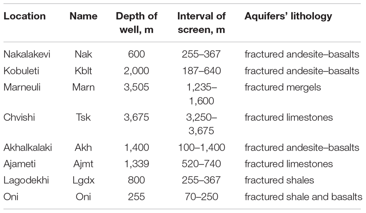
Table 2. Locations and depths of wells in Georgia.
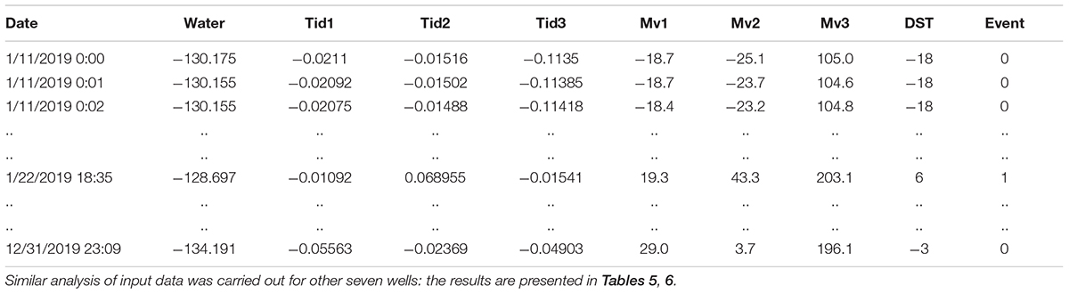
Table 3. One-minute values of predictors and correction factors: water level in the well, tidal variations’ components, magnetic field components, geomagnetic DST index, and EQs.
For the analysis of observed data, we used the algorithm of deep learning ADAM (Kingma and Ba, 2014), which optimizes target function by the combination of the optimization algorithm designed for neural networks (Karpathy, 2017) and a method of stochastic gradient descent with momentum (Bottou and Bousquet, 2012). Our goal is to reveal the change in ML, using statistical characteristics of the time series of Table 3, which precede (here, by 1 day) the occurrence of a seismic event of M3–4; in other words, we consider the next-day EQ forecast problem. In order to apply the ML approach to 1-min observation data (Table 3), it is necessary to transform standard input files into somehow structured data, which permits finding hidden regularities and optimization of prediction. Namely, we calculate for each observation data value (Water, Tid1, Tid2, Tid3, Mv1, Mv2, Mv3, and DST), presented in Table 2 (at a minute count rate), with five statistical functions: Average, Var, SD, Min, and Max. As a result, we obtained Table 4 with dimension 45 × 365 for the mentioned predictors. We also add the 46th column with values 0 or 1 which mark the occurrence (1) or absence (0) of a seismic event in the range M3–4 at the distance of 200 km from the well at a given minute of the year. The catalog used for compilation of the column was from www.emsc-csem.org.
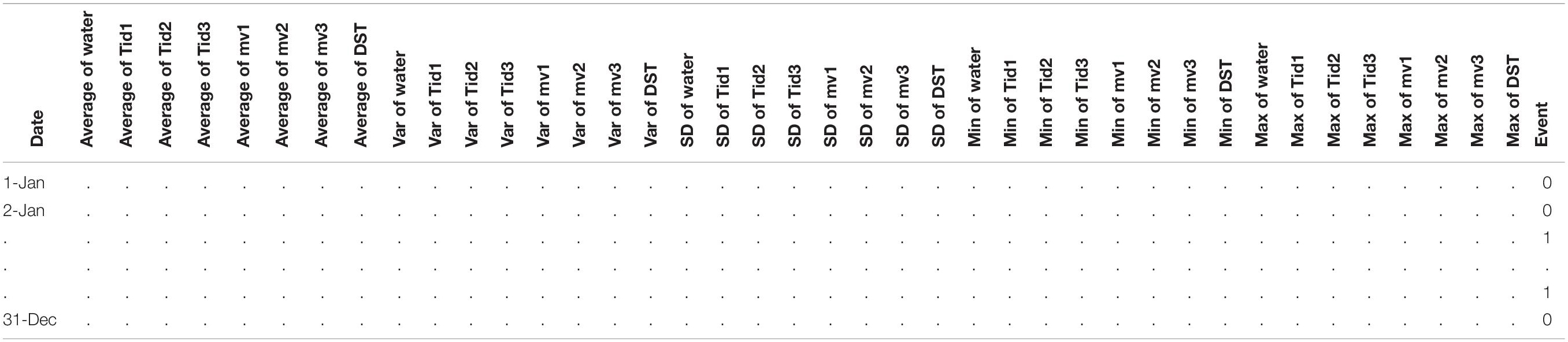
Table 4. Daily values of statistical measures for the complex of predicting fields presented in Table 3.
As a result, we obtained 40 input and one output (target) data for ML. Table 4 is constructed so that a specific day with 40 previously known statistical parameters corresponds to the value of the next day’s event occurrence (0 or 1). We are looking for a functional connection of the previous precursory day data to the next-day seismic event. In other words, the next-day EQ forecast is produced on the basis of statistical analysis of five geophysical variables for the preceding days.
It was interesting to explore the forecasting potential used in ML statistical measures. In Figure 4, we present the weights of such measures, obtained in the process of ML on our 1-day input data for the Ajameti well. We see that in this case the leading factors are the maximal value of the z-component of tidal variation, then followed by, approximately with the same weights, the x-component of magnetic variation and the mean daily value of WL. In general, in all wells, we find six to seven measures, which have the largest weights. This conclusion could change if we include into the input data several preceding days, which we plan to do in the future. The recent paper of Zhang et al. (2019) indicated that the magnitude and phase shift of the tidal response changed significantly after the great Tohoku EQ, so we can expect that a similar effect can take place during EQ preparation.
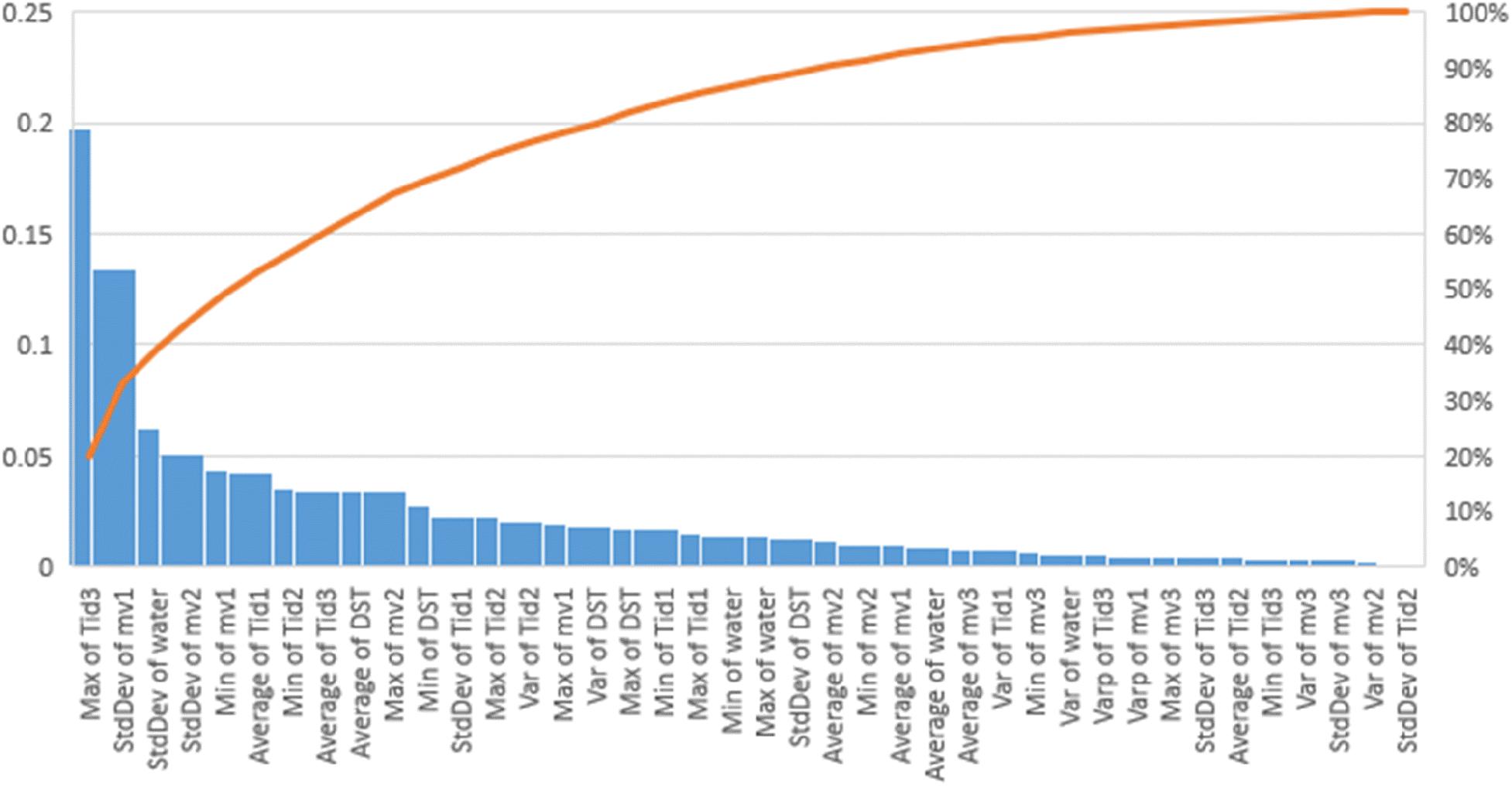
Figure 4. The weights of different statistical measures, obtained in the process of machine learning using input data for the Ajameti well (blue columns). The red curve shows the cumulative percentage of separate weights.
In order to estimate the reliability of the precursors, we used the methodology of receiver operating characteristics (ROC), which is a standard technique for assessing the performance of a binary classifier system (Fawcett, 2006). We are looking for a binary classification (positive p or negative n) of data with four possible outcomes (diagnoses): if the prediction outcome is positive p and the actual value is also p (i.e., the event is correctly predicted), then the outcome is called a true positive (TP) with synonyms sensitivity, recall, and hit rate. If, on the contrary, the diagnosis is positive p and the actual value is n, then the prediction is false positive (FP) with the synonym fallout. Accordingly, when both the diagnosis and the actual value are n, the result is a true negative (TN), and when the prediction outcome is n while the actual value is p, the prediction is classified as a false negative (FN). Using these four diagnoses, the ROC program provides the possibility to calculate the following statistical measures:
Precision = ; Recall = True positive rate (TPR) = ; Accuracy =
False positive rate (FPR) = ; F-measure = F-score = 2 - the harmonic mean of precision and recall: the perfect value of the score is 1, and the worst one is 0.
The K-S statistic is a non-parametric test of the equality of continuous one-dimensional probability distributions that can be used to compare a sample with a reference Kolmogorov–Smirnov probability distribution.
Phi coefficient = (TP ∗ TN - FP ∗ FN)/sqrt[(TP + FP) ∗ (TP + FN) ∗ (TN + FP) ∗ (TN + FN)], which is a correlation coefficient between the observed and predicted binary classifications; it returns a value between + 1 (a perfect prediction) and −1 (total disagreement between prediction and observation).
Lift = [TP/(TP + FP)]/[(TP + FN)/(TP + FP + TN + FN)], which is a measure of the performance of a model at predicting or classifying cases, measuring against a random choice model, i.e., how good it is at identifying the positive (1s) or negative (0s) instances of our dataset.
Kendall’s tau coefficient and Spearman’s rank correlation coefficient (rho) assess Pearson’s correlation between the input values and target values with a difference that the first one works well in the case of linear relationships, whereas the second one is applicable even with non-linear relationships.
ROC AUCH (ROC convex hull) = ROC AUC (area under the ROC curve), which is a performance measure for the ROC classification problem at various thresholds settings. It tells how much the model is capable of distinguishing between classes 1 and 0. The higher the AUC, the better the model predicts 0 as 0 and 1 as 1.
ML Results
The sequence of resources created to generate the deep learning net for all wells (Deepnet) was as follows: Dataset ML_(well name)_2019: 365 instances, 40 fields (1 categorical, 40 numeric); Deepnet ML_(well name)_2019; auto structure suggestion; three hidden layers; ADAM; learning rate = 0.001; beta1 = 0.9; beta2 = 0.999; epsilon = 1e-08; missing values; and max. training time = 1,800. The only parameter which varies for different wells is the number of iterations (indicated for each well separately).
As an example, we show in detail the ML workflow for the 2019 Ajameti well (Figure 5); the number of iterations is 177. Analyzing results presented in Figure 5, we can conclude that the used technique allows next-day forecast (predicting) of 38 EQs (TP) from the total number of 44. Three predictions of event occurrence turn to be false—FP. Seven predictions of the quiet state failed (FN), and 299 of them correctly predicted quietness (TN).
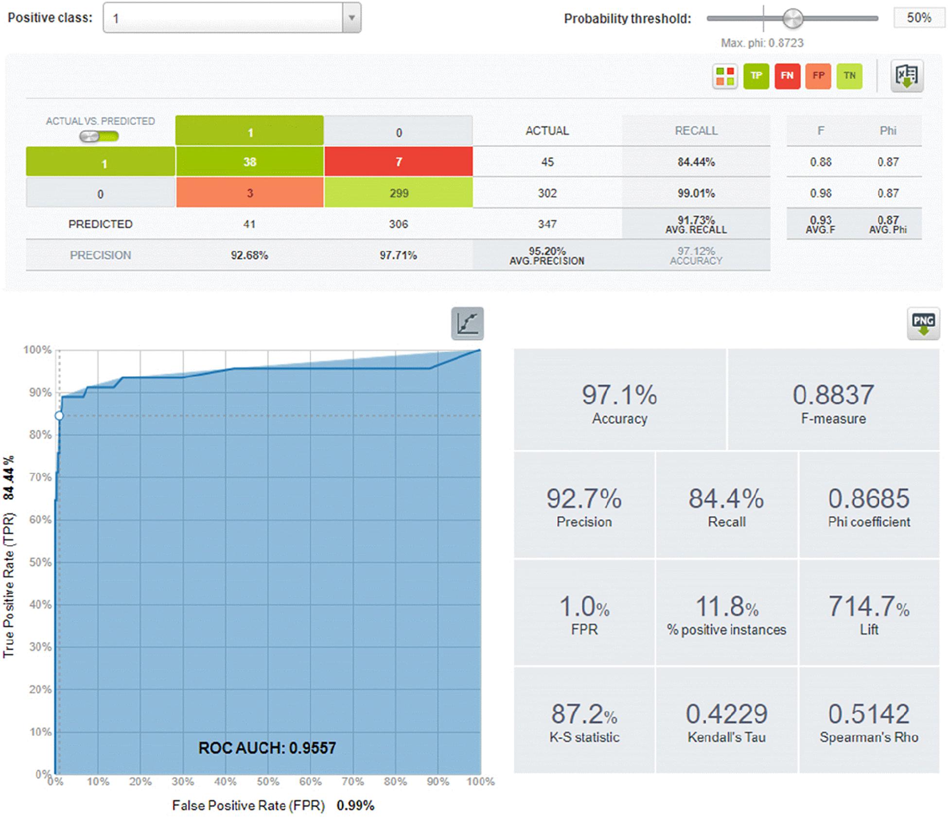
Figure 5. Machine learning and ROC analysis results for 1-year data: next-day M3–4 EQ forecast results for the Ajameti well area (R = 200 km).
According to Table 5 wells allow forecast of next-day EQ with lesser omission. Note that the sum of all ROC values is less than 365, which means that some days’ observations failed. Table 6 contains values of different statistical measures, which we explained above. These data characterize in more detail the different aspects of ADAM algorithm forecasts.
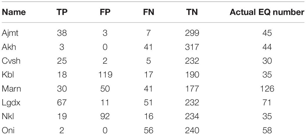
Table 5. ROC values for different wells.
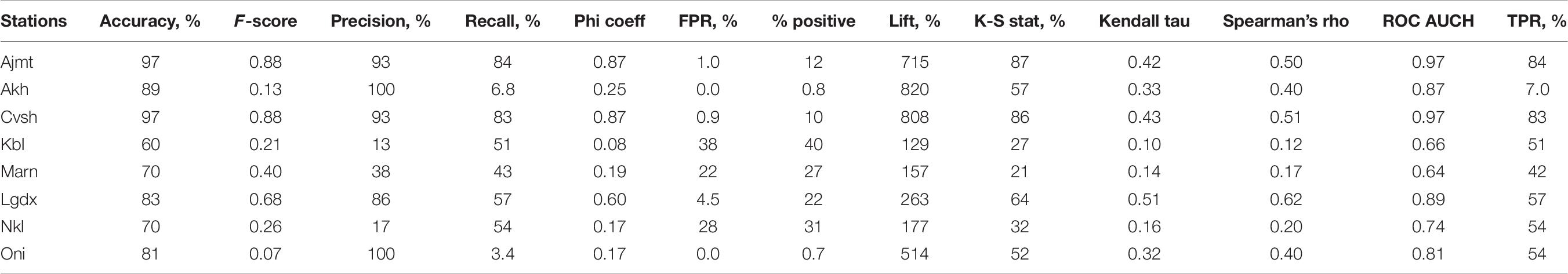
Table 6. Statistical measures of 1-day ROC predictions for different wells.
According to the data presented in Tables 5, 6, five wells (Ajameti, Akhalkalaki, Chvishi, Lagodekhi, and Oni) have good next-day joint EQ/quietness prognostic characteristics (ROC AUCH 0.97–0.81). At the same time, it is necessary to point that due to an overwhelming prevalence of quiet days, even the random prediction of the quiet state is highly successful, and this makes the success of joint prediction very high. We conclude that ROC measures, containing the TN value, increase the joint assessment (ROC AUCH) values. Consequently, the really important measures for the EQ-oriented prediction are “EQ-selective” measures, which do not include TN measures, such as TPR = Recall. In this case, the “best” wells seem to be Ajameti and Chvishi. Note that this conclusion is true only for the next-day forecast—we hope that taking into account input data for several forerunning event days instead of one day can improve the forecasting potential of the used ML algorithm. We cannot exclude also the possibility of different sensitivities of separate wells to pre-seismic deformations, affecting WL in wells.
It is interesting to note that calculated tidal variations reveal high forecasting potential (Figure 3): this can be explained by the indirect effect, the change of the local strain sensitivity of hydraulic properties (permeability and transmissivity) in an aquifer during EQ preparation. Such anomalies were observed by Zhang et al. (2019) after the Tohoku EQ: we presume that similar processes can take place on the preparatory stage of seismic event also.
Next-Day Forecast Testing on the Randomized Events Catalog
In order to assess the reliability of the ML results in the next-day EQ forecast, we distorted the sequence of EQs in the “Events” column in the Table 4 in the following way: the dates of events (EQs) for the time t were displaced in time randomly to positions t + 3 or t + 4. After this, the ADAM algorithm was again used to check the forecast results on the same input data and the randomized EQ sequence.
The results of ML testing on the distorted EQ catalog of Ajameti well data, presented in Tables 6, 7 show that EQ forecast results are negative (TPR, Recall = 0.0%), in contrast to the original data results (Figure 5 and Tables 5, 6). This points to a high accuracy of prediction based on the original data (TPR, Recall = 84%). Namely, all ROC measures, predicting EQ occurrence, have zero values in Tables 7, 8 for randomized data; only quiet days are predicted more or less successfully even in the case of distorted data, which should be expected.

Table 7. ROC values for the randomized EQ catalog—Ajameti well.

Table 8. Statistical measures of the next-day predictions for Ajameti well using randomized EQ catalog.
Future Work
Our short-term forecast analysis was restricted to solving the next-day prediction problem. At the same time, some anomalies are appreciable even visually several days before EQ without complicated analysis (Figure 3). The preliminary results of the quantitative (wavelet) analysis on our data show that the correlation between tidal variations and WL in some wells is broken several days before the local EQs of magnitudes M3–4, in both the amplitude and frequency spectra. We also fixed disturbances of wavelet patterns of magnetic variations in the same periods well before the seismic event. In the future, we are going to apply a detailed ML + ROC analysis to longer (say, several days) prediction intervals and longer series of input data (namely, observation data for dozens of years, prior to 2019), which can improve the results of short-term forecast, in particular, to solve the question on the different prognostic potentials of different wells. In addition, we tried to use a longer prediction interval (10 days) for the Marneuli well, but in this case, the TPR was only 14.5%, i.e., less than the next-day TPR forecast (42%), though the joint EQ/quietness forecast improved significantly (ROC AUCH increased from 42 to 81%). The small TPR effectiveness of the well can be explained by the low sensitivity of the well to EQ-related strains or by another effect, namely, that sometimes a shorter prediction time can be better than a longer one.
Conclusion
We applied several statistical methods to EQ forecast in Caucasus and Georgia and assessed their effectiveness:
(i) Bayesian approach to assess conditional probability of expected strong EQs;
(ii) Pattern recognition technique, based on the assessment of the empirical risk function;
(iii) Non-linear PS plot analysis;
(iv) Machine Learning/Receiver Optimization Characteristic (ML/ROC) algorithms, which show that five wells (Ajameti, Akhalkalaki, Chvishi, Lagodekhi, and Oni) have a good next-day joint EQ/quiet prognostic characteristics (ROC AUCH 0.97–0.81). The other three wells show a less satisfactory result—from 64 to 73%. Our opinion is that due to an overwhelming prevalence of quiet days, even the random prediction of a quiet next-day state is highly successful, and this makes the success of joint EQ/quietness prediction very high due to the large value of the TN term.
Thus, we think that “EQ-aimed” measures, such as TPR = Recall, which do not include the TN measure, are really important for the EQ prediction-oriented studies. In this case, two from the eight wells show good ROC, namely, a high value of the TP EQ prediction (TPR, Recall) of the order of 84–83%; i.e., the next-day impending EQ was predicted from the previously observed data with above-indicated probability. Of course, we cannot exclude the possibility of different sensitivities of separate wells to EQ precursors (different strain sensitivities).
In order to assess the reliability of the ML results in the next-day EQ forecast, we distorted the sequence of EQs in the “Events” sequence and applied the same (ML/ROC) algorithm to the randomized catalog. The results of ML testing on the distorted EQ catalog of Ajameti well data show that EQ forecast results became negative (TPR, Recall = 0.0%), in contrast to the good results obtained for the original data (TPR, Recall = 84–83%).
There is a hope that extending the ML/ROC analysis to longer (say, several days) prediction intervals and longer time series of input data (namely, observation data for dozens of years, prior to 2019) can improve the results of short-term forecast.
Data Availability Statement
The original contributions presented in the study are included in the article/Supplementary Material, further inquiries can be directed to the corresponding author.
Author Contributions
TC contributed to the sections “Introduction,” “Theoretical Models,” “Long-Term and Middle-Term EQ Forecast [Bayesian Approach, Support Vector Machines (SVMs), and Phase Space Portraits (PSPs)],” “Machine Learning (ML) Methodology,” “ML Results,” and “Next-Day Forecast Testing on the Randomized Events Catalog.” GM, GK, and TJ contributed to the sections “Networks, Devices, Data” and “Machine Learning (ML) Methodology.” TK contributed to the sections “Machine Learning (ML) Methodology,” “ML Results,” and “Next-Day Forecast Testing on the Randomized Events Catalog.” All authors contributed to the article and approved the submitted version.
Funding
This work was supported by the Shota Rustaveli National Science Foundation of Georgia (SRNSFG) (FR17_633, study of geodynamical processes evolution and forecasting).
Conflict of Interest
The authors declare that the research was conducted in the absence of any commercial or financial relationships that could be construed as a potential conflict of interest.
Footnotes
References
Adamia, S. H., Alania, V., and Tsereteli, N. (2017). Postcollisional tectonics and seismicity of Georgia. Geol. Soc. Am. Spec. Pap. 525, 535–572. doi: 10.1130/2017.2525(17)
Bender, B., and Perkins, D. M. (1987). Seisrisk III: A Computer Program for Seismic Hazard Estimation. Washington, DC: United States Government Publishing Office.
Bottou, L., and Bousquet, O. (2012). “The tradeoffs of large scale learning,” in Optimization for Machine Learning, eds S. Sra, S. Nowozin, and S. Wright (Cambridge: MIT Press), 351–368.
Brace, W. E., and Byerlee, I. D. (1966). Stick-slip as a mechanism for Earthquakes. Science 153, 990–992. doi: 10.1126/science.153.3739.990
Burges, C. (1998). A tutorial on support vector machines for pattern recognition. Data Min. Knowl. Discov. 2, 121–167.
Burridge, R., and Knopoff, L. (1967). Model and theoretical seismicity. Bull. Seism. Soc. Am. 57, 341–371.
Charmet, J. C., Roux, S., and Guyon, E. (eds) (1990). Disorder and Fracture. NATO ASI Series. Berlin: Springer-Verlag.
Chelidze, T. (1986). Percolation theory as a tool for imitation of fracture process in rocks. PAGEOPH 124, 731–748. doi: 10.1007/bf00879607
Chelidze, T., and Kolesnikov, Y. (1984). On the physical interpretation of transitional amplitude in percolation theory. J.Phys. A 17, L791–L793.
Chelidze, T., Kolesnikov, Y., and Matcharashvili, T. (2006). Seismological criticality concept and percolation model of fracture. Geophys. J. Int. 164, 125–136. doi: 10.1111/j.1365-246x.2005.02818.x
Chelidze, T., and Lursmanashvili, O. (2003). Electromagnetic and mechanical control of slip: laboratory experiments with slider system. Nonlin. Proces. Geophys. 20, 1–8.
Chelidze, T., Lursmanashvili, O., Matcharashvili, T., Varamashvili, N., Zhukova, N., and Mepharidze, E. (2010). “Triggering and synchronization of stick-slip: experiments on spring-slider system,” in Synchronization and Triggering: from Fracture to Earthquake Processes, eds V. de Rubeis, Z. Czechowski, and R. Teisseyre (Berlin: Springer), 123–164. doi: 10.1007/978-3-642-12300-9_8
Chelidze, T., and Matcharashvili, T. (2013). “Triggering and synchronization of seismicity: laboratory and field data- a review,” in Earthquakes - Triggers, Environmental Impact and Potential Hazards, ed. K. Konstantinou (Hauppauge, NY: Nova Science Pub.), 165–231.
Chelidze, T., and Matcharashvili, T. (2015). “Dynamical patterns in seismology,” in Recurrence Quantification Analysis: Theory and best practices, eds C. Webber and N. Marwan (Cham: Springer), 291–335.
Chelidze, T., Matcharashvili, T., and Zhukova, N. (2018). “Phase space portraits of earthquake time series of caucasus: signatures of strong earthquake preparation,” in Complexity of Seismic Time Series, eds T. Chelidze, F. Vallianatos, and L. Telesca (Amsterdam: Elsevier), doi: 10.1016/B978-0-12-813138-1.00001-8
Chelidze, T., Matcharshvili, T., Gogiashvili, J., Lursmanashvili, O., and Devidze, M. (2005). Phase synchronization of slip in laboratory slider system. Nonlin. Process. Geophys. 12, 163–170. doi: 10.5194/npg-12-163-2005
Chelidze, T., Shengelia, I., Zhukova, N., Matcharashvili, T., Melikadze, G., and Kobzev, G. (2016). M9 Tohoku earthquake hydro- and seismic response in the caucasus and North Turkey. Acta Geophys. 64, 567–588. doi: 10.1515/acgeo-2016-0022
Chelidze, T., Sobolev, G., Kolesnikov, Y., and Zavjalov, A. (1995). seismic hazard and earthquake prediction research in georgia. J. Georg. Geophys. Soc. 1A, 7–39.
De Santis, A., Marchetti, D., Pavón-Carrasco, F. J., Cianchini, G., Perrone, L., Abbattista, C., et al. (2019). Precursory worldwide signatures of earthquake occurrences on Swarm satellite data. Sci Rep. 9:20287. doi: 10.1038/s41598-019-56599-1
Diederik, K., and Ba, J. (2014). Adam: a method for stochastic optimization. arXiv [Preprint]. Available online at: https://arxiv.org/abs/1412.6980#:~:text=We%20introduce%20Adam%2C%20an%20algorithm,estimates%20of%20lower%2Dorder%20moments.&text=The%20method%20is%20also%20appropriate,noisy%20and%2For%20sparse%20gradients (accessed June 12, 2020).
Dieterich, J., Cayol, V., and Okubo, P. (2000). The use of earthquake rate changes as a stress meter at Kilauea volcano. Nature 408, 457–460. doi: 10.1038/35044054
Dobrovolsky, I., Zubkov, S., and Miachkin, V. (1979). Estimation of the size of earthquake preparation zones. Pure Appl. Geophys. 117, 1025–1044. doi: 10.1007/bf00876083
Dvorkin, J., Nolen-Hoeksema, R., and Nur, A. (1994). The Squirt-flow mechanism: Macroscopic description. Geophysics 59, 428–438. doi: 10.1190/1.1443605
Fawcett, T. (2006). An Introduction to ROC analysis. Patt. Recogn. Lett. 27, 861–874. doi: 10.1016/j.patrec.2005.10.010
Herrmann, H., and Roux, S. (eds) (1990). Statistical Models For The Fracture Of Disordered Media. Amsterdam: Elsevier.
Jouniaux, L., and Pozzi, J. (1995). Streaming potential and permeability of saturated sandstones under triaxial stress: - consequences for electrotelluric anomalies prior to earthquakes. J. Geophys. Res. 100, 10197–10209. doi: 10.1029/95jb00069
Karpathy, A. (2017). A Peek at Trends in Machine learning. Available online at: https://medium.com/@karpathy/a-peek-at-trends-in-machine-learning-ab8a1085a106 (accessed June 12, 2020).
King, C.-Y., Azuma, S., Ohno, M., Asai, Y., Asai, Y., He, P., et al. (2000). In search of earthquake precursors in the water-level data of 16 closely clustered wells at Tono, Japan. Geophys. J. Int. 143, 469–477. doi: 10.1046/j.1365-246X.2000.01272.x
Kingma, D., and Ba, J. (2014). Adam: A Method for Stochastic Optimization. Available online at: http://arxiv.org/abs/1412.6980http://arxiv.org/abs/1412.6980 (accessed May 12, 2020).
Kopytenko, Y. A., Matiashvily, T. G., Voronov, P. M., Kopytenko, E. A., and Molchanov, O. A. (1990). Discovering of Ultra-Low-Frequency Emissions Connected With Spitak Earthquake and Its Aftershock Activity With the Data of Geomagnetic Pulsations Observations. IZMIRAN, Moscow: Dusheti and Vardzija, 27.
Martinelli, G. (2015). Hydrogeologic and geochemical precursors of earthquakes: an assessment for possible applications. Bollettino di Geofisica Teorica ed Applicata. 56, 83–94.
Matcharashvili, T., Chelidze, T., and Zhukova, N. (2016). Assessment of a ratio of the correlated and uncorrelated waiting times in the Southern California earthquake catalogue. Phys. A 449, 136–144.
McGuire, R. K. (1976). Fortran Computer Program for Seismic Risk Analysis. Reston, VA: U.S. Geological Survey.
Molaie, M., Jafari, S., Moradi, M. H., Sprott, J. C., and Golpayegan, S. (2013). A chaotic viewpoint on noise reduction from respiratory sounds. Biomed. Signal Process. Control. doi: 10.1016/j.bspc.2013.10.009
Nello, C., and Shawe-Taylor, J. (2000). An Introduction to Support Vector Machines and other Kernel-Based Learning Methods. Cambridge: Cambridge University Press.
Ogata, Y. (1998). Space-time point-process models for earthquake occurrences. Ann. Instit. Statist. Math. 50, 379–402. doi: 10.1023/a:1003403601725
Pikovsky, A., Rosenblum, M. G., and Kurths, J. (2003). Synchronization: Universal Concept in Nonlinear Science. Cambridge: CambridgeUniversity Press.
Press, W., Teukmolsky, S., Vetterling, W., and Flannery, B. (2007). Numerical Recipes Art of Scientific computations. Cambridge: Cambridge University Press.
Reasenberg, P., and Matthews, M. (1988). Precursory seismic quiescence: a preliminary assessment of the hypothesis. PAGEOPH 126, 373–406. doi: 10.1007/BF00879004
Reilinger, R., McClusky, S., Vernant, P., Lawrence, S., Ergintav, S., Cakmak, R., et al. (2006). GPS constraints on continental deformation in the Africa-Arabia-Eurasia continental collision zone and implications for the dynamics of plate interactions. J. Geoph. Res. 111:B05411. doi: 10.1029/2005JB004051
Rouet-Leduc, B., Hulbert, C., and Johnson, P. (2019). Continuous chatter of the Cascadia subduction zone revealed by machine learning. Nat. Geosci. 12, 75–79. doi: 10.1038/s41561-018-0274-6
Rouet-Leduc, B., Hulbert, C., Lubbers, N., Barros, K., Humphreys, C., and Johnson, P. (2017). Machine learning predicts laboratory earthquakes. Geophys. Res. Lett. 44, 9276–9282. doi: 10.1002/2017GL074677
Ruina, A. (1983). Slip instability and state variable friction laws. J. Geophys. Res. 88B, 10359–10370. doi: 10.1029/jb088ib12p10359
Saberi, A. (2015). Recent advances in percolation theory and its applications. Phys. Rep. 578, 1–32. doi: 10.1016/j.physrep.2015.03.003
Sobolev, G. (2011). Seismicity dynamics and earthquake predictability. Nat. Hazards Earth Syst. Sci. 11, 445–458. doi: 10.5194/nhess-11-445-2011
Sobolev, G., Chelidze, T., Zavjalov, A., Slavina, L., and Nikoladze, V. (1991). Maps of Expected Earthquakes based on combination of parameters. Tectonophysics 193, 255–265. doi: 10.1016/0040-1951(91)90335-p
Stacey, F. D. (1964). The seismomagnetic effect. Pure Appl. Geophys. 58, 5–22. doi: 10.1007/bf00879136
Stauffer, D., and Aharony, A. (1994). Introduction To Percolation Theory. London: Taylor & Francis, 192.
Theodoridis, S., and Koutroumbas, K. (2009). Pattern Recognition, 4th Edn, Cambridge, MA: Academic Press.
Tsereteli, N., Varazanashvili, O., Kupradze, M., Kvavadze, N., and Gogoladze, Z. (2016). Seismic catalog for Georgia. J. Georg. Geophys. Soc. 19A, 66–74.
Vapnik, V., and Chervonenkis, A. (1974). Pattern Recognition Theory, Statistical Learning Problems. Moskva: Nauka Publisher.
Vapnik V. (ed.) (1984). Algorithms and Programs For Recovering Dependences. Moscow: Nauka Publisher.
Wang, C. Y., and Manga, M. (2009). “Earthquakes and water,” in Encyclopedia of Complexity and Systems, ed. R. A. Maiers (New York, NY: Springer), doi: 10.1007/978-3-642-27737-5_606-1
Zhang, H., Shi, Z., Wang, G., Sun, X., Yan, R., and Liu, C. (2019). Large earthquake reshapes the groundwater flow system: insight from the water-level response to earth tides and atmospheric pressure in a deep well. Water Resour. Res. 55, 4207–4219. doi: 10.1029/2018WR024608
Keywords: Earthquake forecast, phase space portraits, water level in wells, magnetic variations, machine learning, receiver operating characteristic
Citation: Chelidze T, Melikadze G, Kiria T, Jimsheladze T and Kobzev G (2020) Statistical and Non-linear Dynamics Methods of Earthquake Forecast: Application in the Caucasus. Front. Earth Sci. 8:194. doi: 10.3389/feart.2020.00194
Received: 01 April 2020; Accepted: 14 May 2020;
Published: 29 June 2020.
Edited by:
Giovanni Martinelli, National Institute of Geophysics and Volcanology, ItalyReviewed by:
Alexey Lyubushin, Institute of Physics of the Earth (RAS), RussiaGalina Kopylova, Geophysical Survey (RAS), Russia
Copyright © 2020 Chelidze, Melikadze, Kiria, Jimsheladze and Kobzev. This is an open-access article distributed under the terms of the Creative Commons Attribution License (CC BY). The use, distribution or reproduction in other forums is permitted, provided the original author(s) and the copyright owner(s) are credited and that the original publication in this journal is cited, in accordance with accepted academic practice. No use, distribution or reproduction is permitted which does not comply with these terms.
*Correspondence: Tamaz Chelidze, dGFtYXouY2hlbGlkemVAZ21haWwuY29t