 Hoonyoung Jeong
 Alexander Y. Sun4
 Baehyun Min
94% of researchers rate our articles as excellent or good
Learn more about the work of our research integrity team to safeguard the quality of each article we publish.
Find out more
ORIGINAL RESEARCH article
Front. Earth Sci. , 27 May 2020
Sec. Hydrosphere
Volume 8 - 2020 | https://doi.org/10.3389/feart.2020.00108
This article is part of the Research Topic Stochastic Modeling in Hydrogeology View all 11 articles
Ensemble-based stochastic gradient methods, such as the ensemble optimization (EnOpt) method, the simplex gradient (SG) method, and the stochastic simplex approximate gradient (StoSAG) method, approximate the gradient of an objective function using an ensemble of perturbed control vectors. These methods are increasingly used in solving reservoir optimization problems because they are not only easy to parallelize and couple with any simulator but also computationally more efficient than the conventional finite-difference method for gradient calculations. In this work, we show that EnOpt may fail to achieve sufficient improvement of the objective function when the differences between the objective function values of perturbed control variables and their ensemble mean are large. On the basis of the comparison of EnOpt and SG, we propose a hybrid gradient of EnOpt and SG to save on the computational cost of SG. We also suggest practical ways to reduce the computational cost of EnOpt and StoSAG by approximating the objective function values of unperturbed control variables using the values of perturbed ones. We first demonstrate the performance of our improved ensemble schemes using a benchmark problem. Results show that the proposed gradients saved about 30–50% of the computational cost of the same optimization by using EnOpt, SG, and StoSAG. As a real application, we consider pressure management in carbon storage reservoirs, for which brine extraction wells need to be optimally placed to reduce reservoir pressure buildup while maximizing the net present value. Results show that our improved schemes reduce the computational cost significantly.
Since the ensemble Kalman filter was first introduced into the petroleum engineering (Lorentzen et al., 2001; Nævdal et al., 2002; Kim et al., 2018), many ensemble-based history matching methods have gained popularity because they are reduced rank methods (meaning less computational effort) and are relatively easy to implement, parallelize, and couple with any numerical simulator. Chen et al. (2009) first systematically applied the ensemble concept to optimization of well control variables (e.g., well rates and bottom-hole pressures) to maximize the net present value in oil and gas fields. They named their scheme the ensemble optimization (EnOpt) method. Similar to the ensemble-based data assimilation methods, EnOpt can also be easily parallelized and coupled with any simulator.
Another strength of EnOpt is that EnOpt finds an optimal solution under geological uncertainty by maximizing the expectation of the objective function values of multiple models representing model uncertainties, whereas the conventional optimization methods typically require solving each model separately (Chen et al., 2009; van Essen et al., 2009) and optimization under uncertainty is non-trivial (Sun et al., 2013; Zhang et al., 2016). The idea of considering model uncertainties in optimization was also explored by van Essen et al. (2009). van Essen et al. (2009) named their method robust optimization, and the handling of model uncertainties in their method is essentially the same as that in EnOpt. However, EnOpt includes a specific way to compute the gradient, which is needed by all gradient-based optimization algorithms.
The gradient of EnOpt is determined on the basis of the cross covariance between randomly perturbed control variables (or decision variables) and the corresponding objective function values. Because this work is mainly concerned with the gradient approximation in various ensemble methods, hereafter, we will use EnOpt to refer to the gradient approximation in EnOpt where no confusion occurs. Traditional methods for gradient calculation include the finite-difference method (FDM) and adjoint-state method (Sun and Sun, 2015). FDM needs as many objective function evaluations as the product of the number of control variables and the number of ensemble members because FDM perturbs each control variable separately. The adjoint-state method typically requires derivation and solution of a dual problem of the original problem in the adjoint state space, which is not straightforward. In comparison, EnOpt only requires as many objective function evaluations as the number of ensemble members, because it computes the search directions by averaging the objective function anomalies resulting from simultaneous random perturbations of the control vector. Previous studies have shown that the EnOpt can efficiently and satisfactorily achieve improvement of the objective function, despite its low computational cost (Chen et al., 2009; Chen and Oliver, 2010, 2012). However, Fonseca et al. (2017) indicated that EnOpt may not produce satisfactory results for multiple geological models unless the variance in the ensemble models is sufficiently small. The first objective of our work is to show mathematically and experimentally why EnOpt may fail to produce satisfactory results when the variance of the ensemble models is not small.
EnOpt can be considered a variant of the simultaneous perturbation stochastic approximation (SPSA) method introduced by Spall (1992), and SPSA is appropriate for robust optimization because the computational cost of SPSA is significantly lower than that of FDM for a high-dimensional control vector. Even though accurate gradients are obtained using FDM at a high computational cost, gradient-based optimizations are likely to converge to local optima. Rather than spending considerable computational resources computing the gradients, it is more practical to find global optima by trying many initial solutions using the less accurate but more computationally efficient SPSA. SPSA computes the gradient of an objective function more efficiently than FDM does by perturbing control variables randomly and simultaneously (Spall, 1992, 1998). There are several variants of SPSA that can be used to compute the gradient of an objective function stochastically and quickly.
Bangerth et al. (2006) introduced the integer SPSA to solve an optimal well placement problem. Li et al. (2013) applied SPSA for joint optimization of well placement and controls under geological uncertainty. Li and Reynolds (2011) proposed a modification of the SPSA, which is called the stochastic Gaussian search direction (SGSD or G-SPSA). The original SPSA samples perturbations from a symmetric Bernoulli distribution, while SGSD and EnOpt generate perturbations from Gaussian distributions (Chen et al., 2009; Li and Reynolds, 2011). Do and Reynolds (2013) used the simplex gradient (SG) that has the perturbation coefficient of 1 in the formulation of SGSD.
However, Bangerth et al. (2006), Li et al. (2013), Li and Reynolds (2011), and Do and Reynolds (2013) applied the variants of SPSA to optimization of a single geologic model, which means that geological uncertainty was not considered. Fonseca et al. (2017) proposed an extension of SG, which is named the stochastic simplex approximate gradient (StoSAG), that improves the accuracy of the stochastic gradient by repeating multiple perturbations for each ensemble model. In this study, we propose practical ways to reduce the computational cost of EnOpt, SG, and StoSAG by approximating the objective function values of unperturbed control variables using those obtained for the perturbed ones. The proposed approaches reduce about 10% to 50% of the computational cost compared to EnOpt, SG, and StoSAG in our examples.
This paper is organized as follows. In the next section, we explain why EnOpt may fail when the variance of objective function values of the ensemble members is not small, by comparing the gradient approximation schemes in the original EnOpt and SG. Then we propose new hybrid schemes for further reducing computational costs in EnOpt, SG, and StoSAG. Finally, we demonstrate the efficacy of the different schemes using two examples, a test function that is popular for algorithm benchmarking and a well placement optimization problem for pressure management in geologic carbon storage reservoirs.
The steepest ascent or descent algorithm to maximize or minimize an objective function J(u) is given as
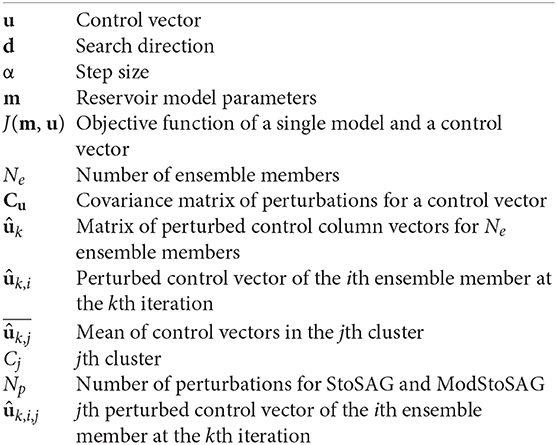
where u is the column vector of control variables; u0 is the initial guess; d is the search direction; α is the step size; and k is an iteration index. For convenience, all major notations used in this study are listed in the Nomenclature table attached at the end of the paper. In this problem, the objective function (J) is dependent only on u. van Essen et al. (2009) replaced J(u) with J(m, u) by adding another input (m) to the scalar function, where m is a random vector generated from a known probability density function. In optimization of well placement and controls, for instance, m may represent uncertain rock properties arising from geologic heterogeneity. J(m, u) is dependent on both m and u, but only u is a control vector. Because J(m, u) inherits the uncertainty of m, van Essen et al. (2009) suggested to maximize the approximate expectation of J(m, u) for mi (i = 1, 2, 3, …, Ne) sampled from a given probability density function (Fonseca et al., 2017).
where and J(mi, u) are called the objective function and the J-function, respectively, to avoid confusion. The former is marginalized over all ensemble members, while the latter corresponds to a single ensemble member.
Ensemble-based gradients (EnOpt, SG, and StoSAG) generate the objective function anomalies by stochastically sampling perturbations for u from a multivariate Gaussian distribution with mean uk and covariance matrix Cu. The perturbed vector of u at the kth iteration is denoted by . In the following, we explain situations that EnOpt may underperform. We then proceed to introduce several hybrid schemes that can significantly reduce the computational costs of the ensemble-based optimization in general while mitigating the underperformance of EnOpt.
SG is given by Do and Reynolds (2013) as.
Equation (3) presented by Do and Reynolds (2013) was applied to a single model. However, once the objective function is replaced with Equation (2) in the formulation of Do and Reynolds (2013), Equation (3) can be applied to multiple models (or robust optimization). Equation (3) is identical to StoSAG with a single repetitive perturbation. Hereafter, we will use SG to refer to StoSAG with a single repetitive perturbation.
The search direction of EnOpt is given by Chen et al. (2009).
Compared to Equation (3), the unperturbed vector of control variables (uk) and the corresponding J(mi, uk) are approximated by their corresponding ensemble means ( and ) in Equation (4) that are further defined as in Equations (5) and (6) (Chen et al., 2009; Do and Reynolds, 2013; Fonseca et al., 2017). In Equation (4), EnOpt needs Ne J-function evaluations to compute a search direction. However, EnOpt requires additional Ne J-function evaluations to calculate the expectation Em[J(m, u)] in Equation (2). In Equations (2) and (4), SG needs 2Ne J-function evaluations to compute a search direction. Thus, SG and EnOpt essentially take the same computational effort (2Ne) to compute a search direction and Em[J(m, u)].
Do and Reynolds (2013) demonstrated that the performances of EnOpt and SG are almost identical for a single geological model. However, Fonseca et al. (2017) pointed out that EnOpt may produce unsatisfactory results because the two assumptions given in Equations (5) and (6) are invalid unless Ne is sufficiently large or the variance in the prior model for m is sufficiently small. Equation (5) is usually valid because perturbations for uk should be sufficiently small to approximate ∇uEm[J(m, u)]. Equation (6) is likely to be invalid if high variations in model parameters such as permeability and porosity cause large variations in J-function values. However, even though the variance of m is small, other variables in the J-function such as unit costs may still make large variations in the J-function values. The claim of Fonseca et al. (2017) can be expressed more quantitatively by simply manipulating Equation (4):
From Equation (7), it follows that
where dk, EnOpt/||dk, EnOpt||∞ ≈ dk, SG/dk, SG||∞ is true if ||rk||2 is sufficiently small compared to dk, SG. However, as ||rk||2 increases, dk, EnOpt becomes more inaccurate than dk, SG. In rk in Equation. (8), because perturbations for uk should be small enough to approximate a search direction accurately, ||rk||2 is significantly dependent on . Thus, ||rk||2 is closely related to the variance in J(m, uk), which is as given in Equation (9):
The norm ||rk||2 is not exactly the same as the variance in J(m, uk), but ||rk||2 is expected to increase as increases because . On the basis of the observation that the approximation of EnOpt becomes inaccurate as the variance in J(mi, uk) increases, we propose a hybrid gradient of EnOpt and SG in the next section that first clusters ensemble members based on the variance of and then approximate J(mi, uk) using within each cluster. Thus, the hybrid gradient is more computationally efficient than SG because the objective function for the unperturbed control vector in some ensemble members does not need to be evaluated. We also propose two additional practical measures that can save the computational cost of EnOpt and StoSAG.
Here, we introduce three new formulations to save on the computational cost of EnOpt, SG, and StoSAG. The new formulations approximate the objective function values for unperturbed control variables using the objective function values for perturbed ones in the formulations of EnOpt, SG, and StoSAG. Thus, these new formulations require fewer J-function evaluations than that by the original ensemble-based gradients.
In EnOpt, the J-function for unperturbed control variables does not need to be evaluated for the search direction, but it needs to be evaluated for the objective function in Equation (2). However, the means of J(mi, uk) and are similar because the perturbations on u are small. Thus, Em[J(m, u)] can be approximated using as given in Equation (10):
We call this the modified EnOpt (ModEnOpt), which uses Equation (10) instead of Equation (2) for approximating Em[J(m, u)]. ModEnOpt requires only half of the number of the J-function evaluations of EnOpt to approximate a search direction and calculate Em[J(m, u)].
To save the computational cost of SG, we propose a hybrid gradient of EnOpt and SG, which is named the hybrid simplex gradient (HSG) method, on the basis of the observation that EnOpt provides satisfactory search directions if the variance in J(m, uk) is small. HSG clusters the ensemble members based on and then uses the cluster mean instead of J(mi, uk) for clusters that have more than one member as given in the first term of Equation (11), which is close to the search direction of EnOpt given in Equation (4). In the second term of Equation (11), J(mi, uk) should be evaluated for the clusters that have only a single member, which is close to the search direction of SG given in Equation (3). The search direction of HSG is given by
HSG uses a different approximation of Em[J(m, u)] given in Equation (12), instead of Equation (2):
In Equation (12), the J-function values for perturbed control variables are used to approximate Em[J(m, u)], but the J-function values for unperturbed ones are used for clusters that have only a single member.
In Equation (11), the Ne ensemble members (models) are grouped based on [J(mi, ûk, i)]. However, determining the optimal number of clusters is still a challenging problem in data clustering (Jain, 2010). Furthermore, even though models are grouped to the optimal number of clusters, some groups might have significantly different values because cluster algorithms group the models into the number of clusters unexceptionally regardless of how similar values are in a group. For this reason, a mean of in a group might not be properly representative of J(mi, uk) of the group members. Thus, rather than trying to determine the optimal number of clusters, we use a predefined criterion to determine if models have similar . A standard deviation is the most common indicator of how dissimilar data are, but the standard deviation should be normalized in our clustering problem. For example, let us assume that there are two data sets (1, 2, 3) and (198, 200, 202). The standard deviation of (1, 2, 3) is smaller than that of (198, 200, 202), but (198, 200, 202) has relatively small differences in terms of magnitude compared to (1, 2, 3). In our clustering problem, group members should have relatively similar J-function values within each group. Thus, for the predefined criterion, we use the coefficient of variation shown in Equation (13) instead of standard deviation to normalize the standard deviation.
Thus, the Ne models are grouped so that the coefficient of variation in each cluster is smaller than a predefined value (CVHSG). However, during clustering, a model should be assigned to a cluster such that the coefficient of variation becomes minimal. We introduce an algorithm to find groups that have small coefficient of variations that are lower than a predefined coefficient of variation. First, Ne models have random cluster indices where the initial number of groups (Nc) is the same to the number of models (Ne). Then whether the coefficient of variation of a group can be reduced by adding a model to the group is examined where the model makes the coefficient of variation of the group minimum. For example, let us assume that we try to select a cluster for a model between clusters A and B. The coefficients of variation of both A and B are smaller than those of CVHSG. If the coefficients of variation of A and B (after including the model) are 0.001 and 0.002, respectively, then the model should be put in cluster A. This is repeated until the coefficient of variation of the group does not become smaller. Finding models that make the coefficient of variation of other groups smaller is repeated. Other details of the proposed algorithm are described in Algorithm 1. In HSG, we use Algorithm 1 to make the coefficients of variation of clusters smaller than CVHSG and to drop the coefficients of variation of clusters. The procedure of clustering is given as follows:
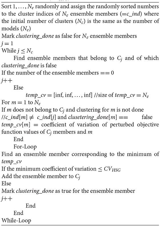
Algorithm 1. Clustering using a predefined coefficient of variations for HSG (CVHSG)
The input of Algorithm 1 includes a predefined coefficient of variation, CVHSG, and the J-function values for perturbed control variables. The number of clusters does not need to be inputted for Algorithm 1. The k-means clustering algorithm (MacQueen, 1967), which is one of the most commonly used clustering algorithms, cannot be used in this case because it requires the number of clusters to be specified and it tends to group members that are relatively close to each other. Determination of the CVHSG value depends on how much computational cost of HSG is expected to be saved compared to SG. For example, if 70% of the computational cost is expected to be saved using HSG compared to SG, then CVHSG is set to a number that makes the number of clusters 70% of the number of ensemble members. CVHSG can be chosen based on the initial J-function values of an ensemble.
HSG is equivalent to ModEnOpt and SG for large and small CVHSG, respectively, where the sum is divided by Ne – 1 in dk, ModEnOpt, but this is canceled by ||dk, ModEnOpt||∞ in Equation (1). For large ||rk||2, a small CVHSG should be used because the approximate gradient of ModEnOpt is inaccurate. HSG takes Ne ~ 2Ne J-function evaluations where Ne and 2Ne correspond to the number of J-function evaluations of ModEnOpt and SG, respectively.
The search direction of StoSAG is given by Fonseca et al. (2017) as
StoSAG repeats multiple perturbations (Np) for each ensemble member, while SG takes a single perturbation for each ensemble member. StoSAG provides more accurate search directions than SG does because StoSAG takes more J-function evaluations to compute the search direction than SG. StoSAG needs Ne(Np + 1) J-function evaluations, and this is (Np + 1)/2 times as many J-function evaluations as SG requires.
The computational cost of StoSAG can be reduced by approximating the J-function values of unperturbed control variables using the J-function values of perturbed ones as given below:
The modified StoSAG (ModStoSAG) uses different approximations of Em[J(m, u)] given in Equation (17) instead of Equation (2):
ModStoSAG requires NeNp J-function evaluations, and it can save 1/(Np + 1) of the computational cost of StoSAG needed to compute a search direction. A summary of the ensemble-based stochastic gradient methods discussed thus far is presented in Table 1. ModEnOpt, HSG, and ModStoSAG use different objective functions, but the objective function in Equation (2) is calculated at initial and final steps for all the formulations to compare them in the next numerical examples.
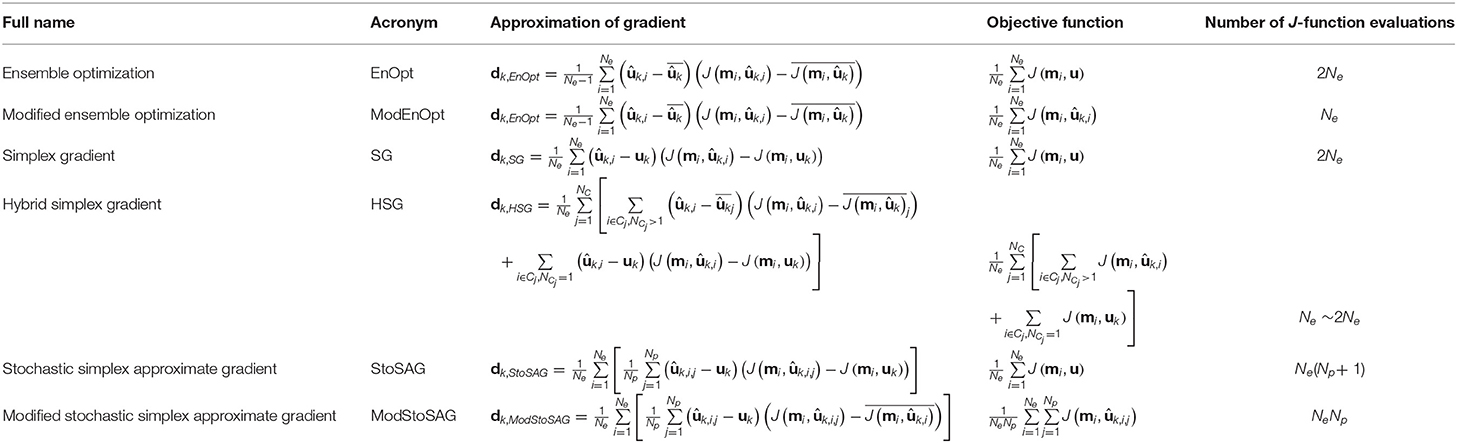
Table 1. Names, formulas, and number of objective function evaluations of six formulations.
The performance of the six formulations given in Table 1 is tested using the Rosenbrock (1960) function, which is widely used for benchmarking optimization solvers. The Rosenbrock function is given by
where and i = 1, 2, …, Ne. mi is a constant (=100) in the original Rosenbrock function, but ensemble members have different mi to mimic geological uncertainty where . The number of ensemble members is 100 (Ne = 100), and the ensemble members have different mi. The dimension of u is 50, and an initial solution is ui = 2.0 for i = 1, 2, …, Nu. The objective function is in Equation (19), and 100 J-function evaluations are needed to calculate the objective function. Two values of σm (0.01 and 1.00) are used to generate two sets of m1, m2, …, m100 for the 100 ensemble members. A larger σm makes a larger variance in J(mi, u) and larger ||rk||2, which causes inaccurate search directions of EnOpt and ModEnOpt. Perturbations for u are generated using N(0, Cu) where Cu is a diagonal matrix and the diagonal elements are 0.0012. Np is set to 3 for both StoSAG and ModStoSAG.
CVHSG is set to a number that makes the number of clusters about 70 (=0.7 · 100). CVHSG for σm = 0.01 and 1.00 are 1E−5 and 5E−5, respectively, which were determined based on the J-function values for the initial solution (ui = 2.0 for i = 1, 2, …, Nu).
The performance of the stochastic gradients is compared to the gradient obtained using FDM (Sun and Sun, 2015). A search direction of FDM is computed using Equation (20), and Ne(Nu + 1) function evaluations are needed.
The optimization problem is solved using the steepest descent method given in Equation (1). The optimization is terminated if either of the following two conditions is satisfied: (i) the relative increase of the objective function is <0.0001%, or (ii) the relative change of the norm of uk – uk+1 is <0.01%.
Figure 1 shows the optimization results for σm = 0.01. Figures 1A,B show the results of a single run and the average result of 100 runs, respectively. Because perturbations are stochastically generated for the stochastic gradients (EnOpt, ModEnOpt, SG, HSG, StoSAG, and ModStoSAG), the optimization runs using the stochastic gradients show the different numbers of J-function evaluations and relative objective function values for iterations. For this reason, in Figure 1B, the 100 optimization runs are repeated, and the relative objective function values and the total number of J-function evaluations are averaged for each iteration. In Figure 1, because σm (=0.01) is small, the variance in J(mi, u) is also small, and the small variance in J(mi, u) leads to small ||rk||2. Because EnOpt and ModEnOpt provide accurate search directions for small ||rk||2, EnOpt and ModEnOpt find satisfactory solutions as the other gradient methods do.
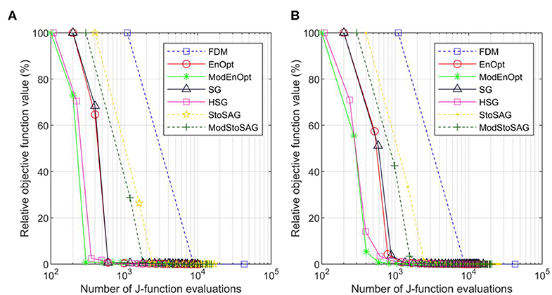
Figure 1. Plot of numbers of J-function evaluations and relative objective function values of the seven gradient methods for σm = 0.01. (A) Relative objective function value is a percentage of the initial objective function value. Symbols represent iterations, and the x-axis is the total number of function evaluations. (B) Shows the average relative objective function values and the average total number of function evaluations of 100 optimization runs.
Table 2 shows the numbers of function evaluations that are needed to achieve 5% of the relative objective function value in Figure 1B. ModEnOpt, HSG, and ModStoSAG saved about 47, 33, and 34% of the function evaluations compared to EnOpt, SG, and StoSAG, respectively. In Table 2, ModEnOpt took the smallest number of function evaluations, and EnOpt needed a smaller number of function evaluations than SG did.
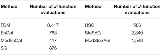
Table 2. Numbers of function evaluations that are needed to achieve 5% of the relative objective function value in Figure 1B.
However, EnOpt and ModEnOpt do not achieve satisfactory reduction of the objective function value for σm = 1.0 as shown in Figure 2A. In Figure 2B, EnOpt and ModEnOpt show the abnormal relation between the number of J-function evaluations and relative objective function values because EnOpt and ModEnOpt do not reduce the objective function value sufficiently for all the 100 optimization runs. The large σm(=1.0) results in a large variance in J(mi, u) and, consequently, large ||rk||2. For this reason, EnOpt and ModEnOpt provide inaccurate search directions and unsatisfactory optimization results. The average angles between the search directions obtained using FDM and the stochastic gradients for σm = 1.0 are given in Table 3. The angle between two search direction vectors is calculated using Equation (21):
where u and v are vectors corresponding to search directions. The angle calculations are repeated 100 times and averaged. The search direction obtained using FDM is considered to be the most accurate, and a higher angle from the FDM search direction implies less accuracy. It can be seen from Table 3 that SG, HSG, StoSAG, and ModStoSAG provide acceptable search directions, while EnOpt and ModEnOpt provide inaccurate search directions. The number of J-function evaluations for the same relative objective value increases from HSG, SG, ModStoSAG, and StoSAG, as shown in Figure 2B.
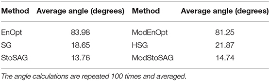
Table 3. Average angles between the search directions obtained using FDM and the stochastic gradients for σm = 1.0.
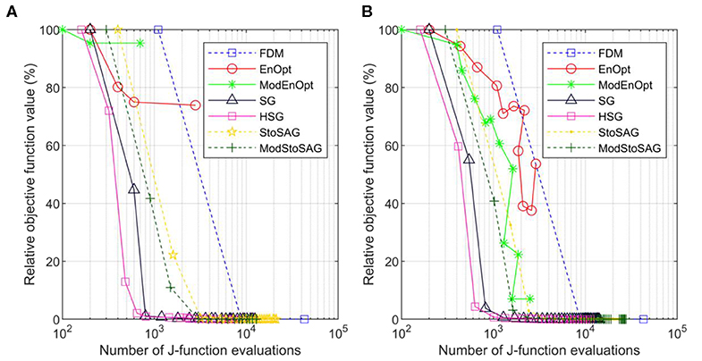
Figure 2. Plot of numbers of J-function evaluations and relative objective function values of the seven gradient methods for σm = 1. (A) Relative objective function value is a percentage of the initial objective function value. Symbols represent iterations, and the x-axis is the total number of function evaluations. (B) Shows the average relative objective function values and the average total number of function evaluations of 100 optimization runs.
As a realistic example, we now consider the optimization of brine extraction well placement in geological carbon sequestration (GCS) applications. CO2 injection into saline aquifers or depleted oil and gas reservoirs necessarily leads to pore pressure increases. The pore pressure buildup not only can affect the CO2 injectivity and storage performance but may also cause caprock damage, fault reactivation, induced seismicity, and leakage of brine and CO2, posing severe problems to CO2 long-term storage permanence and public safety (Birkholzer et al., 2012; Carroll et al., 2014; Cihan et al., 2015). Recently, active reservoir pressure management was proposed as a mitigation measure, which installs one or more brine extraction wells to reduce pressure buildup in the reservoir (Bergmo et al., 2011; Buscheck et al., 2011, 2012; Birkholzer et al., 2012; Cihan et al., 2015; Arena et al., 2017). The extraction, treatment, and disposal of the extracted brine, however, impose additional expenses to GCS operators (Cihan et al., 2015). Thus, the placement and control of brine extraction wells need to be optimized to improve the economic feasibility of GCS projects. Cihan et al. (2015) optimized well placement and controls of brine extraction wells in different geological models to minimize extracted brine volume and keep pressure buildups under critical thresholds for potentially activating fault leakage and/or fault slippage. In their study, Cihan et al. (2015) adopted a constrained differential evolution algorithm, which is a heuristic stochastic evolution algorithm similar to the genetic algorithm. Here, we demonstrate the use of the more efficient ensemble-based gradient algorithms. Optimal placement of a brine extraction well is sought in multiple geological models (i.e., geologic uncertainty) to maximize the objective function, which is expressed in the form of the net present value. Performance of the six formulations given in Table 1 is compared.
The J-function for a single model, mi, is given by
where the control vector u is a two-dimensional column vector including I and J indices of brine extraction wells. In words, the objective function in Equation (22) can be described as the tax credit for injected CO2 minus the penalty for unfulfilled CO2 injection, the cost of brine extraction wells, and the damage cost related to brine and CO2 leakage.
The brine extraction wells are vertically perforated in a CO2 injection zone, and I and J indices are rounded off to integers during iterations. Δtn is the size (days) of the nth time step in the reservoir simulation, and b is the annual discount rate. Ninj, Next, and Nleak are the numbers of CO2 injection, brine extraction, and leaky wells, respectively. , , and represent the average CO2 injection rate at the jth CO2 injector, the average brine extraction rate at the kth brine extractor, and the average CO2 extraction rate at the kth brine extractor for Δtn, respectively.
One of the main risks related to GCS is leakage from abandoned wells—if abandoned wells are leaky, then brine and CO2 can migrate to an overlying formation along the leaky wells (Birkholzer et al., 2012; Sun et al., 2013). Because the risk related to leakage must be minimized for safe long-term CO2 storage, abandoned wells are assumed to be leaky for conservative estimation. In Equation (20), and are the brine leakage rate at the lth leaky abandoned well and the CO2 leakage rate at the lth leaky abandoned well for the nth time step. If brine extraction wells are placed near the leaky wells, the brine and CO2 leakage amount decreases because the installed brine extraction wells reduce the pressure buildup at the leaky wells; on the flip side, the brine extraction wells also need to be shut in early if they are placed near CO2 injectors because they have early CO2 breakthroughs. The brine extraction wells should be placed at locations that minimize the leakage costs at the leaky wells while postponing CO2 breakthrough at the brine extraction wells as late as possible. rci is the credit for CO2 storage, which is often provided by the government subsidy or driven by the carbon trading market (Jahangiri and Zhang, 2012; Allen et al., 2017). In Equation (23), is the minimum required CO2 injection rate for Δtn, and a penalty is imposed when the injection rate cannot be met, , in which case the upstream capturing facility needs to find an alternative means for temporary storage. In Equation (20), cbe, cce, cbl, and ccl are the unit costs of brine treatment, CO2 reinjection, brine leakage, and CO2 leakage, respectively.
Overall, the brine extraction well placement optimization is complex, especially when geologic uncertainty is involved. The ensemble gradient methods are well-suited to solve such problems because of their efficiency and the ability to incorporate geologic uncertainty. As a demonstration, we consider the three-dimensional reservoir model shown in Figure 3, which is 2.55 km (x-axis) by 2.55 km (y-axis) by 30 m (z-axis), and the dimensions of a grid block are 50 m by 50 m by 10 m. The vertical structure consists of three formations, which are named the above zone, caprock, and injection zone. CO2 is injected at 30 tons/day at the center of the injection zone for 5 years, and the maximum bottom-hole pressure is 20,000 kPa. Brine is extracted at an extraction well at 60 m3/day, and it is shut in if the ratio of produced CO2 volume to produced brine volume is >100. The caprock blocks the flow between the above and injection zones, but brine and CO2 can vertically flow up along two leaky abandoned wells where the leaky wells are located 300 m north and east of the injector in Figure 4. The unit cost data needed for calculating the J-function in Equations (22) and (23) are given in Table 4.
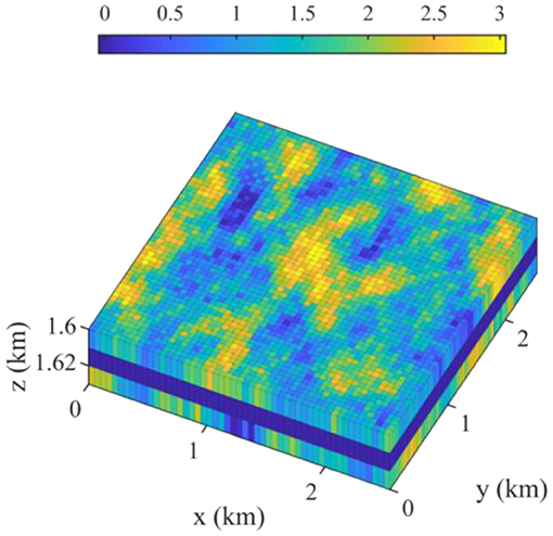
Figure 3. Three-dimensional view of log10 permeability (md). The z-axis is exaggerated by a factor of 20.
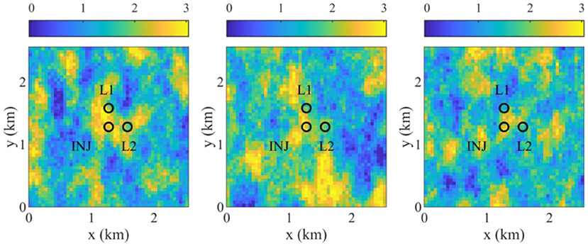
Figure 4. Top view of log10 permeability (md) of 3 of 20 geological models, and the locations of an injector (INJ) and two leaky abandoned wells (L1 and L2).
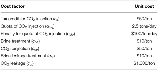
Table 4. Cost factors and unit costs for brine extraction.
Heterogeneous porosity and log10 permeability fields are generated using the sequential Gaussian simulation and the sequential Gaussian co-simulation modules of SGeMS (Remy et al., 2011). Porosity and log10 permeability follow normal distributions, and their statistical parameters are given in Table 5. Figure 4 shows three realizations of log10 permeability out of a total of 20 geological models. The porosity and permeability of the caprock zone are assumed deterministic and are assigned values of 0.1 and 0.001 md, respectively. The flow simulation is conducted using a compositional multiphase reservoir simulator, CMG-GEM (CMG, 2015). The two leaky abandoned wells are described using the local grid refinement of CMG-GEM, and the porosity and the vertical permeability of the leaky wells are set to 0.2 and 1,000 md.
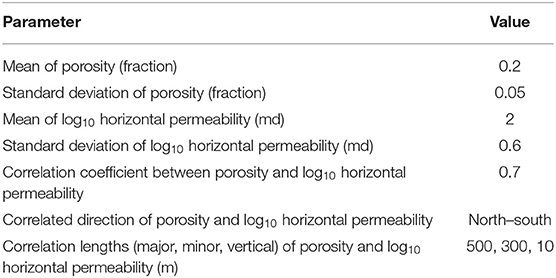
Table 5. Statistical parameters used to generate the geological model.
The convergence criteria are as follows: (i) the relative increase of the objective function is <0.1%, or (ii) the relative change of the norm of uk – uk+1 is <1%.
The objective of this optimization problem is to find the optimal location of a brine extraction well that maximizes the mean of the J-function values given in Equation (22) of the 20 geological models. As described in Equation (22), a solution for a brine extraction well is a two-dimensional vector including I and J indices of the brine extraction well. Thus, in this example, the vector of a search direction has two elements for the I and J indices of a brine extraction well, and the I and J indices of a solution are updated at the same time using the search direction. The optimal solution is sought using the six stochastic gradients, and then the performance of the six stochastic gradients is compared. In HSG, CVHSG is set to a number that makes the number of clusters about 80% of the number of ensemble members. Np = 2 is used for StoSAG and ModStoSAG.
Figure 5 shows the brine extraction well locations at the iterations obtained using HSG for four different initial solutions. In general, initial solutions for optimization are sampled in a prior distribution, but the initial solutions located at the four corners in Figure 5 are selected because optimal solutions are expected to be located between CO2 plume and the boundary. The four different initial solutions are fixed to compare the performance of the stochastic gradients. As described in the previous section, a brine extraction well should be placed as close to the CO2 injector and the leaky wells as possible to mitigate the reservoir pressure buildup, as well as CO2 and brine leakage amounts. However, the brine extraction well is shut in early if the brine extraction well is placed in the extent of the CO2 plume, which changes for different brine extraction well locations because the CO2 migration is affected by the reservoir pressure drawdown caused by the brine extraction well. Furthermore, the reservoir pressure buildup and drawdown, the CO2 and brine leakage amounts, and the CO2 plume extent are significantly affected by the heterogeneity of rock permeability in the 20 geological models. As shown in Figure 6, a brine extraction well should be placed out of the CO2 plume extent and as close to the CO2 injector and the leaky wells. (11, 11) and (40, 11) shown in Figures 5C,D are converged to the same solution, which is (31, 18) shown in Figure 6.
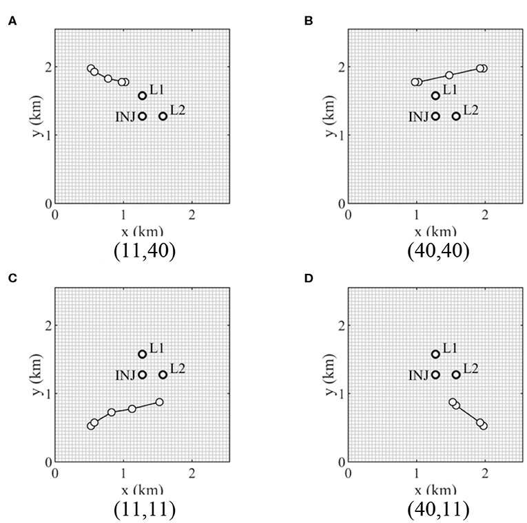
Figure 5. Iteration steps of well placement of a brine extraction well using HSG for four initial solutions (I and J indices). INJ and L1 and L2 represent the CO2 injector and two leaky abandoned wells, respectively. (A) 1st initial solution (11,40). (B) 2nd initial solution (40,40). (C) 3rd initial solution (11,11). (D) 4th initial solution (40,11).
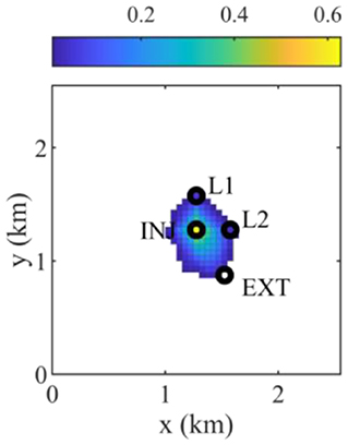
Figure 6. Average CO2 saturation map of 20 geological models after CO2 is injected for 5 years when placing a brine extraction well at the optimal location (I = 31 and J = 18). INJ, EXT, and L1 and L2 represent the CO2 injector, the brine extraction well, and two leaky abandoned wells, respectively.
Figure 7 shows the numbers of simulation runs and objective function values of the six stochastic gradient methods for four initial solutions. In Figure 7, the number of simulation runs is how many times the flow simulator is conducted until an iteration is finished. For example, if the suite of the 20 models is simulated five times until an iteration ends, then the number of simulation runs is 100.
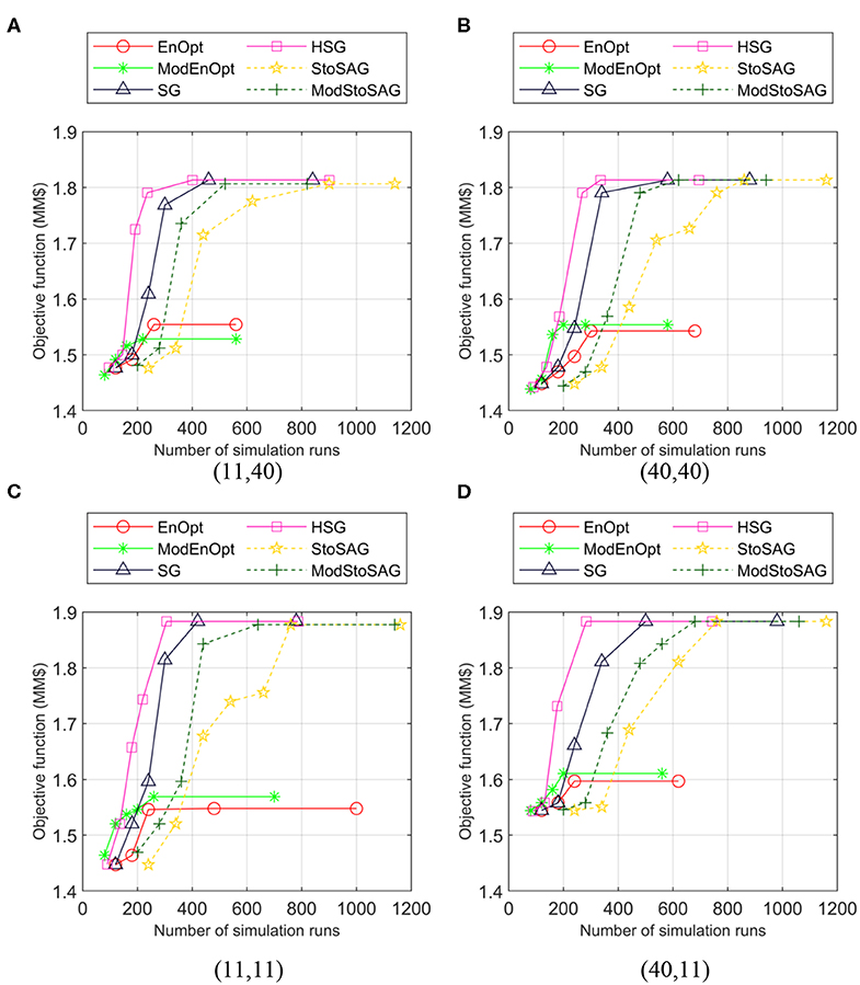
Figure 7. Plot of numbers of simulation runs and objective function values of the six stochastic gradient methods for four initial solutions (I and J locations). Symbols represent iterations, and the x-axis is the total number of simulation runs. (A) 1st initial solution (11,40). (B) 2nd initial solution (40,40). (C) 3rd initial solution (11,11). (D) 4th initial solution (40,11).
EnOpt and ModEnOpt do not achieve satisfactory objective function values compared to the others. This implies that in Equation (8) or the variance in J(mi, u) is too large for EnOpt and ModEnOpt to provide acceptable accuracy of search directions. In Figure 7, for the same number of simulation runs, HSG and ModStoSAG reach higher objective function values than SG and StoSAG do.
Ensemble-based optimization algorithms are widely used for reducing the computational costs of optimization, especially when the forward problem requires a significant amount of time to run. In this work, we theoretically and experimentally showed when EnOpt may fail to achieve satisfactory performance. If in Equation (8) or the variance in J(mi, u) is large, EnOpt produces unsatisfactory optimization results because the search direction of EnOpt is inaccurate as shown in the Rosenbrock function example. We also introduced hybrid schemes to reduce the computational costs of EnOpt, SG, and StoSAG. For the benchmark example and the geological carbon sequestration example, the computational costs of EnOpt, SG, and StoSAG can be significantly reduced by replacing the J-function values for the unperturbed control variables with those for the perturbed ones. The ensemble-based optimization schemes proposed in this study are generic and can be readily used on other types of problems involving computationally expensive forward simulations or optimization under uncertainty.
The datasets generated for this study will not be made publicly available. It is a confidential data set. Requests to access the datasets should be directed to the corresponding author.
HJ was a main author to make research results and wrote this manuscript. HJ had technical discussions with AS, JJ, BM, and DJ.
HJ was supported by the National Research Foundation of Korea (NRF) under grant number 2018R1C1B5045260, and the Korea Institute of Geoscience and Mineral Resources(KIGAM) and the Ministry of Science, ICT and Future Planning of Korea under grant number GP2020-006. AS was supported by the U.S. Department of Energy, National Energy Technology Laboratory (NETL) under grant number DE-FE0026515. BM was supported by the National Research Foundation of Korea (NRF) under grant numbers 2018R1A6A1A08025520 and 2019R1C1C1002574.
The authors declare that the research was conducted in the absence of any commercial or financial relationships that could be construed as a potential conflict of interest.
Allen, R., Nilsen, H. M., Andersen, O., and Lie, K.-A. (2017). On obtaining optimal well rates and placement for CO2 storage. Comput. Geosci. 21, 1403–1422. doi: 10.1007/s10596-017-9631-6
Arena, J. T., Jain, J. C., Lopano, C. L., Hakala, J. A., Bartholomew, T. V., Mauter, M. S., et al. (2017). Management and dewatering of brines extracted from geologic carbon storage sites. Int. J. Greenh. Gas Control 63, 194–214. doi: 10.1016/j.ijggc.2017.03.032
Bangerth, W., Klie, H., Wheeler, M. F., Stoffa, P. L., and Sen, M. K. (2006). On optimization algorithms for the reservoir oil well placement problem. Comput. Geosci. 10, 303–319. doi: 10.1007/s10596-006-9025-7
Bergmo, P. E. S., Grimstad, A.-A., and Lindeberg, E. (2011). Simultaneous CO2 injection and water production to optimise aquifer storage capacity. Int. J. Greenh. Gas Control 5, 555–564. doi: 10.1016/j.ijggc.2010.09.002
Birkholzer, J. T., Cihan, A., and Zhou, Q. (2012). Impact-driven pressure management via targeted brine extraction—conceptual studies of CO2 storage in saline formations. Int. J. Greenh. Gas Control 7, 168–180. doi: 10.1016/j.ijggc.2012.01.001
Buscheck, T. A., Sun, Y., Chen, M., Hao, Y., Wolery, T. J., Bourcier, W. L., et al. (2012). Active CO2 reservoir management for carbon storage: Analysis of operational strategies to relieve pressure buildup and improve injectivity. Int. J. Greenh. Gas Control 6, 230–245. doi: 10.1016/j.ijggc.2011.11.007
Buscheck, T. A., Sun, Y., Hao, Y., Wolery, T. J., Bourcier, W., Tompson, A. F. B., et al. (2011). Combining brine extraction, desalination, and residual-brine reinjection with CO2 storage in saline formations: Implications for pressure management, capacity, and risk mitigation. Energy Procedia 4, 4283–4290. doi: 10.1016/j.egypro.2011.02.378
Carroll, S. A., Keating, E., Mansoor, K., Dai, Z., Sun, Y., Trainor-Guitton, W., et al. (2014). Key factors for determining groundwater impacts due to leakage from geologic carbon sequestration reservoirs. Int. J. Greenh. Gas Control 29, 153–168. doi: 10.1016/j.ijggc.2014.07.007
Chen, Y., and Oliver, D. S. (2010). Ensemble-based closed-loop optimization applied to Brugge field. SPE Reserv. Eval. Eng. 13, 56–71. doi: 10.2118/118926-PA
Chen, Y., and Oliver, D. S. (2012). Localization of ensemble-based control-setting updates for production optimization. SPE J. 17, 122–136. doi: 10.2118/125042-PA
Chen, Y., Oliver, D. S., and Zhang, D. (2009). Efficient ensemble-based closed-loop production optimization. SPE J. 14, 634–645. doi: 10.2118/112873-PA
Cihan, A., Birkholzer, J. T., and Bianchi, M. (2015). Optimal well placement and brine extraction for pressure management during CO2 sequestration. Int. J. Greenh. Gas Control 42, 175–187. doi: 10.1016/j.ijggc.2015.07.025
Do, S. T., and Reynolds, A. C. (2013). Theoretical connections between optimization algorithms based on an approximate gradient. Comput. Geosci. 17, 959–973. doi: 10.1007/s10596-013-9368-9
Fonseca, R. R.-M., Chen, B., Jansen, J. D., and Reynolds, A. (2017). A stochastic simplex approximate gradient (StoSAG) for optimization under uncertainty. Int. J. Numer. Methods Eng. 109, 1756–1776. doi: 10.1002/nme.5342
Jahangiri, H. R., and Zhang, D. (2012). Ensemble based co-optimization of carbon dioxide sequestration and enhanced oil recovery. Int. J. Greenh. Gas Control 8, 22–33. doi: 10.1016/j.ijggc.2012.01.013
Jain, A. K. (2010). Data clustering: 50 years beyond K-means. Pattern Recognit. Lett. 31, 651–666. doi: 10.1016/j.patrec.2009.09.011
Kim, S., Min, B., Lee, K., and Jeong, H. (2018). Integration of an iterative update of sparse geologic dictionaries with ES-MDA for history matching of channelized reservoirs. Geofluids 2018, 1–21. doi: 10.1155/2018/1532868
Li, G., and Reynolds, A. C. (2011). Uncertainty quantification of reservoir performance predictions using a stochastic optimization algorithm. Comput. Geosci. 15, 451–462. doi: 10.1007/s10596-010-9214-2
Li, L., Jafarpour, B., and Mohammad-Khaninezhad, M. R. (2013). A simultaneous perturbation stochastic approximation algorithm for coupled well placement and control optimization under geologic uncertainty. Comput. Geosci. 17, 167–188. doi: 10.1007/s10596-012-9323-1
Lorentzen, R. J., Fjelde, K. K., Frøyen, J., Lage, A. C. V. M., Nævdal, G., and Vefring, E. H. (2001). “Underbalanced and low-head drilling operations: real time interpretation of measured data and operational support,” in SPE Annual Technical Conference and Exhibition (New Orleans, LA: Society of Petroleum Engineers).
MacQueen, J. (1967). “Some methods for classification and analysis of multivariate observations,” in Proceedings of the Fifth Berkeley Symposium on Mathematical Statistics and Probability (Berkeley, CA).
Nævdal, G., Trond, M., and Vefring, E. H. (2002). “Near-well reservoir monitoring through ensemble kalman Fflter,” in SPE/DOE Improved Oil Recovery Symposium (Tulsa, OK: Society of Petroleum Engineers).
Remy, N., Boucher, A., and Wu, J. (2011). Applied Geostatistics With SGeMS: A User's Guide. Cambridge University Press. Available online at: https://books.google.com/books/about/Applied_Geostatistics_with_SGeMS.html?id=eSxstwAACAAJ&pgis=1 (accessed August 14, 2015).
Rosenbrock, H. H. (1960). An automatic method for finding the greatest or least value of a function. Comput. J. 3, 175–184. doi: 10.1093/comjnl/3.3.175
Spall, J. C. (1992). Multivariate stochastic approximation using a simultaneous perturbation gradient approximation. IEEE Trans. Automat. Contr. 37, 332–341. doi: 10.1109/9.119632
Spall, J. C. (1998). Implementation of the simultaneous perturbation algorithm for stochastic optimization. IEEE Trans. Aerosp. Electron. Syst. 34, 817–823. doi: 10.1109/7.705889
Sun, A. Y., Nicot, J.-P., and Zhang, X. (2013). Optimal design of pressure-based, leakage detection monitoring networks for geologic carbon sequestration repositories. Int. J. Greenh. Gas Control 19, 251–261. doi: 10.1016/j.ijggc.2013.09.005
Sun, N.-Z., and Sun, A. (2015). Model Calibration and Parameter Estimation: For Environmental and Water Resource Systems. New York, NY: Springer.
van Essen, G., Zandvliet, M., van den Hof, P., Bosgra, O., and Jansen, J.-D. (2009). Robust waterflooding optimization of multiple geological scenarios. SPE J. 14, 202–210. doi: 10.2118/102913-PA
Zhang, X., Sun, A. Y., and Duncan, I. J. (2016). Shale gas wastewater management under uncertainty. J. Environ. Manage. 165, 188–198. doi: 10.1016/j.jenvman.2015.09.038
Keywords: stochastic gradient, ensemble optimization, simplex gradient, stochastic simplex approximate gradient, hybrid simplex gradient, active pressure management
Citation: Jeong H, Sun AY, Jeon J, Min B and Jeong D (2020) Efficient Ensemble-Based Stochastic Gradient Methods for Optimization Under Geological Uncertainty. Front. Earth Sci. 8:108. doi: 10.3389/feart.2020.00108
Received: 24 December 2019; Accepted: 24 March 2020;
Published: 27 May 2020.
Edited by:
Liangping Li, South Dakota School of Mines and Technology, United StatesReviewed by:
Xiaodong Luo, NORCE Norwegian Research Centre, NorwayCopyright © 2020 Jeong, Sun, Jeon, Min and Jeong. This is an open-access article distributed under the terms of the Creative Commons Attribution License (CC BY). The use, distribution or reproduction in other forums is permitted, provided the original author(s) and the copyright owner(s) are credited and that the original publication in this journal is cited, in accordance with accepted academic practice. No use, distribution or reproduction is permitted which does not comply with these terms.
*Correspondence: Hoonyoung Jeong, aG9vbnlvdW5nLmplb25nQHNudS5hYy5rcg==
Disclaimer: All claims expressed in this article are solely those of the authors and do not necessarily represent those of their affiliated organizations, or those of the publisher, the editors and the reviewers. Any product that may be evaluated in this article or claim that may be made by its manufacturer is not guaranteed or endorsed by the publisher.
Research integrity at Frontiers
Learn more about the work of our research integrity team to safeguard the quality of each article we publish.