 Paolo Piras1†
 Antonio Profico2
 Luca Pandolfi3
 Pasquale Raia4*
 Fabio Di Vincenzo5,6
 Alessandro Mondanaro3,4
 Silvia Castiglione4Valerio Varano7†
- 1Department of Scienze Cardiovascolari, Respiratorie, Nefrologiche, Anestesiologiche e Geriatriche, Sapienza Università di Roma, Rome, Italy
- 2PalaeoHub, Department of Archaeology, University of York, York, United Kingdom
- 3Department of Earth Science, University of Florence, Florence, Italy
- 4Department of Earth Sciences, Environmental and Resources, University of Naples “Federico II”, Naples, Italy
- 5Department of Environmental Biology, Sapienza University of Rome, Rome, Italy
- 6Italian Institute of Human Palaeontology (IsIPU), Anagni, Italy
- 7Department of Architecture, Roma Tre University, Rome, Italy
In modern shape analysis, deformation is quantified in different ways depending on the algorithms used and on the scale at which it is evaluated. While global affine and non-affine deformation components can be decoupled and computed using a variety of methods, the very local deformation can be considered, infinitesimally, as an affine deformation. The deformation gradient tensor F can be computed locally using a direct calculation by exploiting triangulation or tetrahedralization structures or by locally evaluating the first derivative of an appropriate interpolation function mapping the global deformation from the undeformed to the deformed state. A suitable function is represented by the thin plate spline (TPS) that separates affine from non-affine deformation components. F, also known as Jacobian matrix, encodes both the locally affine deformation and local rotation. This implies that it should be used for visualizing primary strain directions (PSDs) and deformation ellipses and ellipsoids on the target configuration. Using C = FTF allows, instead, one to compute PSD and to visualize them on the source configuration. Moreover, C allows the computation of the strain energy that can be evaluated and mapped locally at any point of a body using an interpolation function. In addition, it is possible, by exploiting the second-order Jacobian, to calculate the amount of the non-affine deformation in the neighborhood of the evaluation point by computing the body bending energy density encoded in the deformation. In this contribution, we present (i) the main computational methods for evaluating local deformation metrics, (ii) a number of different strategies to visualize them on both undeformed and deformed configurations, and (iii) the potential pitfalls in ignoring the actual three-dimensional nature of F when it is evaluated along a surface identified by a triangulation in three dimensions.
Introduction
Modern shape analysis exploits the potential of specific computational algorithms applied to phenomena where the deformation and/or the variation of shapes are under investigation. In geometrical terms, shapes are represented by vectors of point coordinates (=landmarks) that can be compared by means of different mathematical formalisms. In shape analysis, the term “shape” is referred to forms (intended as shape+size) that have been standardized at unit size that can be quantified in various ways (see below). Prior to computing any kind of shape distance or deformation estimation, two or more shapes are commonly “superimposed” to filter out information relative to position, rotation, and, optionally, size, which do not represent intrinsic shape variation. At this point, two principal cases must be distinguished:
i) Shapes are identified by clouds of points without any specific correspondence/homology.
ii) Shapes are defined by landmarks that are anatomically or topologically homologous across different configurations (=points correspondence).
As for the first case, while most applications, from biology (Adams et al., 2013) to paleontology (Piras et al., 2010) to medicine (Piras et al., 2019), usually analyze shapes and forms by using homologous anatomical landmarks, the use of continuous surfaces without points correspondence is faced by exploiting the potential of a plethora of diffeomorphic techniques not treated in detail here (see Trouvé, 1998; Durrleman et al., 2012). Briefly, when using these diffeomorphic techniques, shapes are considered as images (2D) or surfaces (3D) that are registered using different algorithms (Ceritoglu et al., 2013): diffeomorphic approaches are used for this purpose such as large diffeomorphic deformation metric mapping (LDDMM; Miller et al., 2014, 2015) that represents, today, one of the most used (among many others) approaches for estimating shape differences, surface matching, and Parallel Transport of deformations (Charlier et al., 2017). In this context, size is more frequently quantified using m-Volume.
In the second case, one of the most used approaches to align a shape onto another is ordinary Procrustes analysis (OPA; Gower, 1975). If multiple shapes are to be analyzed, their consensus landmark configuration (=grand mean) is computed by applying the generalized Procrustes analysis (GPA; Gower, 1975; Rohlf and Slice, 1990). OPA and GPA can be performed with or without scaling landmark configurations to unit size, the latter being usually represented by centroid size (CS, the square root of sum of squared distance between landmark's configuration and their centroid). Scaling or not scaling shapes at unit CS leads to different Riemannian manifolds (size- and shape-space or shape-space; Dryden and Mardia, 2016) described by different metrics and possessing different geometrical properties (Le, 1988). The Riemannian manifolds are curved spaces that can be considered as the multidimensional generalization of a curved surface. Shape-spaces are particular Riemannian spaces whose points represent shapes. In general, shape-spaces are not representable pictorially except for the shape-space case of three landmarks in two dimensions where the manifold is a sphere where shapes live under the same equivalence classes of rotation translation and size (defined as CS).
OPA and GPA translate all shapes imposing their centroids on the origin of axes and rotating them to minimize the Procrustes distance D as defined as in Equation (1):
where X and Y represent two centered, aligned, and scaled configurations; k is the number of landmarks; and m is the number of dimensions. D is a geodesic distance that is often linearized by orthogonally projecting it in the plane tangent to the consensus. After GPA, common ordination methods, such as principal component analysis (PCA), are frequently applied in order to find directions of variations. This workflow is routinely applied in Geometric Morphometrics (GM; Bookstein, 1991; Claude, 2008; Zelditch et al., 2012; Dryden and Mardia, 2016).
In this article, we focus on those applications where point homology/correspondence is assumed (i). In the case of two aligned shapes or of a PCA performed on a collection of shapes either, the notion of deformation always pertains to a pair of shapes, i.e., a source (X: the “undeformed” shape that can be a real shape or a sample's consensus) and a target (Y: representing the deformation of the source, i.e., a real shape or a shape predicted by an ordination axis). Recently, several contributions focused on the visualization of deformations by using different kinds of local measures from infinitesimal local area changes (Márquez et al., 2012, 2014) to velocity fields of local deformations (Kratz et al., 2013). Locally (see below), tensors are used to quantify local deformation. The choice to visualize a unique particular metric extracted from a tensor inevitably implies a certain loss of information even in the simplest case of local affine deformation of finite elements (FE) that are usually triangular in 2D or tetrahedral (less commonly cubic) in 3D (tetrahedral FE structures will be treated here). Márquez et al. (2012) showed the importance of the evaluation, quantification, and statistical assessment of local deformation in GM examples coming from evolutionary biology. GM is being routinely used to address a wide spectrum of hypotheses. In particular, the use of shape analysis has been fruitfully coupled with phylogenetic comparative methods in order to explore patterns of convergence/divergence (Stayton, 2015; Castiglione et al., 2019), morphospace occupation (Santos et al., 2019), morphological integration (Piras et al., 2014; Sansalone et al., 2019), functional hypothesis (Oxnard and O'Higgins, 2009), and developmental growth (Angulo-Bedoya et al., 2019; Colangelo et al., 2019). All these studies share the same basic source of phenomenological interpretation: the shape change studied via shape analysis (very often GM). The importance to evaluate more quantitatively the local deformation stems from the fact that it allows a statistical treatment of shape variation (Márquez et al., 2012).
In this paper, we aim to describe and discuss the principal strategies available for computation of local deformation and its visualization for paleontologists and evolutionary biologists that usually use shape analysis in their investigations. We also present the very basic mathematical details underlying analytical machinery encoded in common shape analysis practice coupled with essential notions of continuum mechanics related to the estimation of local deformation. In particular we (i) describe the main analytical basis for the quantification of local deformation; (ii) illustrate and, in some cases, implement the main options and metrics for visualizing it on both 2D and 3D objects; (iii) illustrate an important feature of deformation in 3D when the shapes are represented by triangular surfaces having only a “shell” structure rather than a volumetric appearance; and (iv) present some applications in both 2D and 3D paleontological case studies.
We also provide (as Supplementary Material) fully reproducible codes in R with all necessary ad hoc built functions aimed at reproducing any figure and analysis presented in the paper.
Computation Methods
Deformation Gradient Tensors at Local Scale
The main statement of the present paper is related to the concept of local deformation that is always considered, infinitesimally, as an affine transformation even when the global transformation affecting the source shape is not (Figure 1). For simplicity, we will use here the term affine as a synonym of uniform and linear deformation. In fact, one gets linear deformations by removing translations from affine deformations. Uniform means that the gradient of the deformation (the local strain, see below) is constant. At the same time, we will use non-uniform as a synonym of non-linear and non-affine. In the first example, we consider the non-affine deformation affecting a square grid in Figure 1. Infinitesimally, each square sub-element of the grid experiences an affine transformation that deforms it into a parallelogram. In ℝ2 (i.e., in two-dimensions), the neighborhood around every point of a square can be mapped onto a different one by a linear transformation represented by a 2 × 2 matrix. We would deal with 3 × 3 matrix in ℝ3 (i.e., in three dimensions). In particular, it is possible to transform a point of coordinates p ≡ (x, y) into an infinitesimally deformed one of coordinates p + u ≡ (x,y) + (ux,uy) = (x + ux,y + uy) with the displacement vector field u ≡ (ux, uy) through the displacement gradient tensor
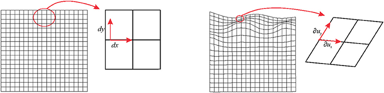
Figure 1. Left panel: a non-affine deformation of a regular square. Right panel: a global non-affine deformation is shown. Infinitesimally, the deformation can be considered as linear.
If we add the identity matrix I, we obtain the deformation gradient tensor
Denoting X the k × m matrix, with k the number of landmarks and m the number of dimensions, of an undeformed configuration (here we refer to the small squared cell of the grid), we can obtain Y as linear transformation of X using
With “T” the transpose symbol.
The same holds in ℝ3 by adding the z-coordinate to the system.
F encodes deformation + rotation, and these two aspects can be decoupled by computing a polar decomposition of F.
with R the m × m rotation matrix encoded in F and
with
C is symmetric and positive definite. The very nature of C is that it encodes exclusively the local deformation on the source without rotation. It can be used to perform an eigenvalue decomposition obtaining v and λ, i.e., the eigenvectors and the corresponding eigenvalues; λ is the collection of m eigenvalues usually returned in decreasing order, while v is its corresponding collection of m vectors each with m components. It must be noted that R resulting from the polar decomposition of F is not equal to the rotation found during OPA for the minimization of D. Varano et al. (2018, section 4.3) distinguish the two rotations by unifying OPA and modified OPA (MOPA) in one formalism. Moreover, R has a local meaning and can be different at any chosen evaluation point while when two configurations are superimposed, a global rotation is found.
It is not uncommon, in GM studies, to interpret the local deformation of a given target (w.r.t. a source) as the collection of displacement vectors of landmarks identifying the configurations. This practice inevitably leads to a misconception of what local deformation actually is and, consequently, to a misinterpretation of the process underlying observed shapes. Figure 2 shows this point by starting with a simple rotation (first row, left panel) of a square X with coordinates x1(−0.5,0.5), x2(0.5,0.5), x3(0.5,0.5), x4(−0.5,0.5) that does not encode a shape deformation but that presents non-null displacements (blue arrows). When applying a shear + rotation–deformation using F = , we can show that F and C (which are constant in the case of affine transformations), evaluated at target and source vertices, respectively, do not follow displacements in any way (first row, right panel and second row, left panel). Even removing global rotation using OPA, displacements do not bear the same meaning of deformation ellipses. In this particular case, OPA and MOPA coincide: the two rotations, in fact, coincide if we found UXTX = XTXU with U defined in Equation (6). This is the same as saying that the principal axes of X have the same directions as the principal strains of F. A square is also a particular case as the inertia tensor XTX is spherical and does not have principal axes. In the case of two generic shapes, a source and a target linked by a non-affine transformation, OPA and MOPA lead to different global alignments (Figure 2, third row). The same effects are evident also in the case of non-affine transformations. Figure 3 shows a simple bilinear transformation that deforms the same square as in Figure 2 into a trapezoid with coordinates x′1(−1,0.25), x′2(1,0.25), x′3(0.3,0.25), x′4(−0.3,0.25). Rotation is not present in this transformation, and the two shapes are then intrinsically aligned. C and F were evaluated at source and target vertices, respectively. Displacements, again, cannot be considered as proxies of local deformation mainly for landmarks 1 and 2 (= at the square base). It is thus important to underline that during OPA, position and rotation (as well as optionally size) are removed globally. Locally, rotations are still present and the relationship between local deformation and displacements depends on the infinitesimal differences among displacements as encoded in the displacement gradient tensor H. When dealing with shapes more complex than the platonic ones shown here, things become more complex, and it is necessary to carefully look at local deformations and displacements in the correct way (see real examples below). F maps infinitesimal deformations between the reference and target configurations by measuring the rate of shape deformation at any point along all directions simultaneously. It is also known in literature as Jacobian matrix (Márquez et al., 2012). In this paper, we consider F as a synonym of Jacobian matrix and its determinant indicates the ratio between target and source m-Volumes, i.e., the infinitesimal change in m-Volume in the neighborhood of the point where F is evaluated.
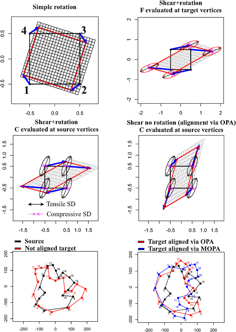
Figure 2. Relationship between displacement vectors (in blue) and local deformations as depicted using (on the source) or F (on the target). First row, left panel: a simple rotation that produces displacements without deformation; first row, right panel: a shear+rotation with deformation ellipses evaluated at target vertices; second row, left panel: the same shear+rotation with deformation ellipses evaluated at source vertices; second row, left panel: the same shear without global rotation (filtered out via OPA) with deformation ellipses evaluated at source vertices; third row, left panel: a generic source (in black) and a non-aligned generic target (in red); third row, right panel: plot with source and the target aligned using OPA (in red) or MOPA (in blue). Principal strain directions (=ellipse's axes) are in black if tensile and in violet if compressive.
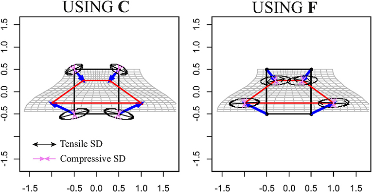
Figure 3. Left panel: a bilinear transformation deforms the regular square into a trapezoid; was used to compute local deformations at source vertices with displacement vectors (in blue). Right panel: the same with deformation ellipses evaluated on the target using F. Principal strain directions (=ellipse's axes) are in black if tensile and in violet if compressive.
While the explanation above refers to the general continuous case, F and C can be obtained in the discrete case using alternative ways. In this paper, we propose two approaches:
a) Direct calculation: the simplest case to illustrate this is the case of two triangles X and Y as illustrated in Figure 4. Triangles are the most used basic geometries in 2D FE analysis, and they can experience only affine transformations. For this reason, they are used for mesh generation (as done in this paper) in order to evaluate F within a larger body (see below). We calculate the covariant basis a1 and a2 on X as the vector differences between two vertices p1 and p2 and X centroid (c) and their normal vector a3.
we can use a3 in order to obtain the contravariant basiss
The covariant basis in Y is as followss
F is obtained as
This workflow is valid for triangles in both ℝ2 and ℝ3. For tetrahedra in ℝ3, the workflow is pretty similar with the inclusion of the calculation of a third axis corresponding to the tetrahedron's face not lying along the plane identified by three landmarks belonging to the tetrahedron.
b) Evaluation of the deformation gradient tensor F starting from a global interpolating function that models the deformation of X to obtain Y.
A convenient interpolant is represented by the thin plate spline (TPS), a special case of kriging (Kent and Mardia, 1994). TPS is the most used interpolation function in biological and paleobiological investigations that exploit modern shape analysis potential.
X and Y can be complex bodies constituted by homologous landmarks within which we evaluate F locally at any desired point (thus not by using the direct calculation on mesh triangle's centroids) starting from TPS coefficients.
The landmark-wise representation of TPS (Dryden and Mardia, 2016, Equation 12.8) is
with εm being the m-dimensional Euclidean space, c is a point of εm represented by an m × 1 matrix, A is a linear transformation of εm represented by an m × m matrix, W is a k × m matrix representing the non-affine component (Dryden and Mardia, 2016; see below), and s is a k × 1 matrix s(x) = (σ(x – x1)… σ(x – xk))T with:
Using the shape-wise representation, where a configuration is defined in the configuration space (with k the number of landmarks and m the number of dimensions), we have:
where lk is a column vector of ones of length k.
TPS finds the best functions by minimizing the cost function bending energy
where ν = 16 for m = 2 and ν = 8 for m = 3 (see Varano et al., 2017). This corresponds to the integral
This represents a mean elastic energy evaluated on the whole ℝm as the effect of the non-affine part of the deformation ψ (Bookstein, 1989).
The usefulness of TPS is that it separates the global affine part from the non-affine one. XAT in Equation (10) represents the affine part of the transformation with A an m × m matrix that corresponds exactly to F in the special case of a uniform deformation applied to X. Varano et al. (2018) argued that while XAT ⊥ W, it is not orthogonal to SW (i.e., the non-affine part of the deformation). S is the k × k matrix where the biharmonic function σ(h) is evaluated on the source configuration and
With Γ11 being the bending energy matrix (see Dryden and Mardia, 2016) estimated upon X.
Varano et al. (2018) proposed different methods and strategies to calculate the affine component even while using the TPS by exploiting the so-called “TPS space” (Varano et al., 2017, 2018). For the same reason, Rohlf and Bookstein (2003) added to the existing method proposed in Bookstein (1996) two new methods for computing the affine component in a transformation: (i) the complement of the space of pure bending shape variation and (ii) the regression method. These two methods do not require the reference configuration to be aligned to its principal axes. While the former implies the computation of the bending energy matrix, the latter does not and can be easily implemented using the computation of the pseudoinverse matrix in a linear system relating the source and the target configurations. This solution is the same as the least squares estimator when the aim is the estimation of the affine transformation between a source and a target shape.
When evaluating infinitesimally the gradient of the deformation estimated by the TPS, namely, Ftps, we always obtain a linear transformation as, infinitesimally, all transformations become linear.
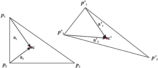
Figure 4. Left panel: an undeformed triangle. Right panel: its deformed state. Axes used for deriving F are shown. c, centroid.
Figure 5 summarizes the main concept briefly exposed in this section.
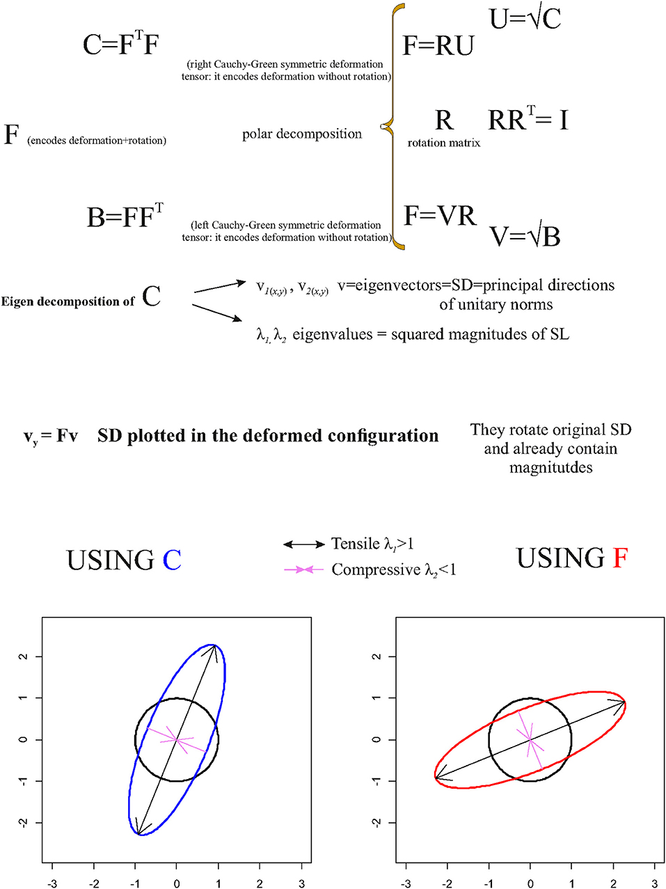
Figure 5. Synthetic illustration showing the very basic mathematical relationship between F, C, and R as well as the geometrical meaning of v and vy.
Computationally, Ftps can be derived as follows:
– Given a pair of shapes X(the undeformed) and Y (the deformed), one can compute A, W, and S using Equation (10), yielding the best interpolant ψ.
– The gradient of the interpolant is the map: ∇ψ: εm → Mm × m associating to each point n ϵ εm the Mm × m matrix resulting from the sum of A in Equation (10) with the product between the m × k matrix W T in Equation (10) and the k × m matrix ∇s containing the first partial derivatives of the biharmonic function evaluated on each point n.
Specifically in 2D:
With first partial derivatives:
And in 3D
With first partial derivatives:
Where
While ∇(ψ) informs about the deformation directions and magnitudes at evaluation points, one could be interested in the local changes of these directions and magnitudes. This means computing the second-order gradient deformation tensor ∇∇(ψ) that allows to quantify the amount of local bending energy stored in the deformation. ∇∇(ψ) has m × (m × m) components. It is convenient to represent these components in matrix format. In particular, we represent ∇∇(ψ)n as the product of an m × k matrix with a k × (m × m) matrix with n the point where ∇∇(ψ) is evaluated.
For 2D problems we have:
With second partial derivatives:
Where
In 3D, we have:
With second partial derivatives:
Where
||∇∇(ψ)||2 represents just J(ψ) presented in Equation (12) when it is evaluated on whole ℝm. Locally, can be interpreted as the bending energy density, i.e., how much is non-affine (=non constant) local deformation in the neighborhood of n where it has been evaluated. Moreover, in the presence of an FE mesh, it can be evaluated at centroids of each element and multiplied by the element's m-Volume to compute, in a discrete way, the body bending energy JΩ that has an important mechanical meaning in the decomposition of deformation and for its relationship with the strain energy φ (see below). Varano et al. (2018) provided a detailed description of the relationship between J, JΩ, and ϕ and their importance in computing the direct transport, i.e., the parallel transport the TPS space (Varano et al., 2017, 2018).
In particular,
gives the decay index Varano et al. (2018), i.e., the ratio between bending energy computed on whole Rm and on the body only. Recently, Varano et al. (2019) proposed the construction of the body bending energy matrix BΩ in order to restrict it exclusively within the physical boundaries of objects involved in the deformation analysis.
The bending energy can be considered as a pseudo-distance as it vanishes for globally affine transformations. A more physical distance, used in continuum mechanics, that vanishes on the rotational part of the local deformation, is the complete strain energy:
where μ and λ are the Lamé elastic moduli, related to the material properties of the body, and
is the strain tensor (for small displacement). In the case of pure geometrical structures, μ and λ are immaterial and we could adopt a simplified expression for the strain energy:
As already stated for body bending energy, this strain energy becomes an energy density when evaluated infinitesimally at specific locations.
Principal Strain Directions, Deformation Ellipses, and Ellipsoids
One can use v and λ in order to depict deformation directions of a unitary circumference (in 2D) or a sphere (in 3D) as shown in Figure 5, conveniently rescaled if necessary, and the principal axes of the resulting ellipses (or ellipsoids in ℝ3).
The principal axes identify the (reciprocally) orthogonal principal strain direction (SD) given by v while λ gives their squared magnitudes.
As stated above, C does not encode rotation; thus, , v, and λ must be used in order to map SD, and to depict deformation ellipses or ellipsoids, on the source shape; in order to depict this information on the target shape using SD encoded in v, v must be pre-multiplied by F in order to depict SD on the target configuration such as
vy already encodes SD magnitudes. This procedure rotates v within the target according to R encoded in F.
SD possesses an important deformational and mechanical meaning when computed on deformed shapes that are the result of specific forces such as in the left ventricle contraction (Evangelista et al., 2015; Gabriele et al., 2016; Piras et al., 2017; Varano et al., 2018). λi = 1 indicates no deformation, λi > 1 indicates a deformation that produces an expansion (=tensile SD) along the direction of the corresponding SD, while λi < 1 indicates a deformation that produces a compression (=compressive SD). The closer the λi to 1, the smaller is the deformation. This means that in case of λi > 1 or λi < 1, the direction of maximal deformation is dictated by the v corresponding to the λi most distant from 1:
The corresponding direction of maximal deformation (either tensile or compressive) , on the source, or on the target, is often called primary strain direction (PSD).
We recall here that we are dealing with locally affine transformations. In case of direct calculation (see above) made on single triangular (or tetrahedral) FE of a Delaunay triangulation computed within two general X and Y shapes, these FEs should not be re-aligned via OPA. Accordingly, if using Ftps, one should use Ctps = Ftps and for deforming unitary circumference or sphere on the source and vytps = Ftpsvtps and Ftps for plotting them on the target. Figure 6 illustrates a square that is deformed in a parallelogram using the tensor = . Using either the direct calculation or TPS interpolation in ℝ2, F is fully recovered. One can use F or in order to depict the deformation ellipse and corresponding SD on target or source configuration, respectively.
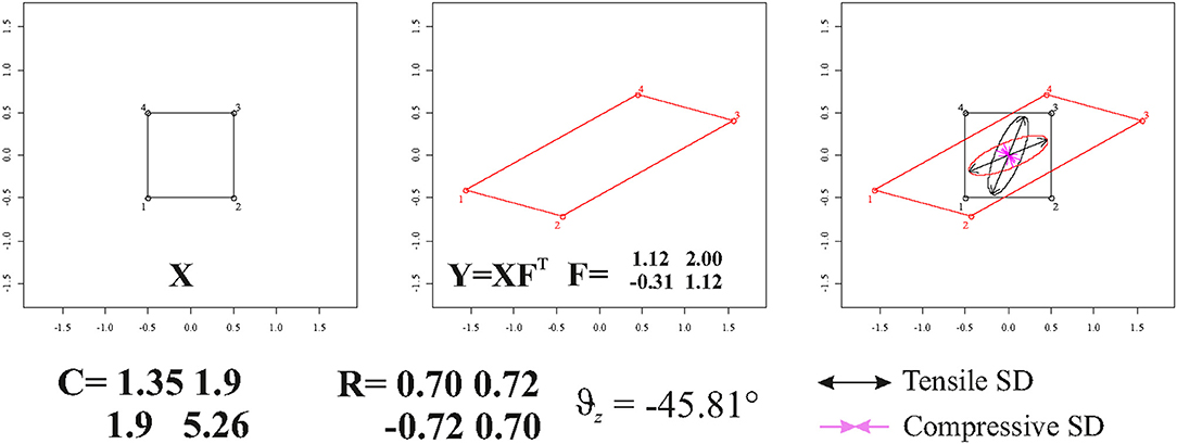
Figure 6. The deformation of a square in a parallelogram and SD plotted on source and target configurations. C, F, and Θz are also shown.
Choosing Evaluation Points and Their Visualization
The concept of “localness” inevitably implies the choice of a series of evaluation points within the geometry subjected to a deformation. One of the most effective approaches, widely applied over a large spectrum of applications, is the Delaunay triangulation (Márquez et al., 2014; Dryden and Mardia, 2016). The construction of the triangulation proceeds iteratively by choosing the centroids of the initial sets of defined triangles as a new set of triangle's vertices. In this manner, an unlimited number of triangles can be assembled. Specifically, the constrained Delaunay triangulation allows limiting the construction of the triangulation itself exclusively within the body of interest by providing proper contour information in 2D and surface in 3D. Once a criterion to choose deformation gradient evaluation points is established (i.e., constrained Delaunay), it is essential to have also a criterion to locate them in both source and target configurations as homologous points. While this could be of lesser importance in non-biological applications, it is instead mandatory to have them as much as possible anatomically homologous when dealing with biological structures. Whereas, the homology of a point, in a biological structure, is an elusive concept (as a point is dimensionless; Bookstein, 1991; Dryden and Mardia, 2016), it is nevertheless approached in those cases where histological delimitations are visible, for example, at the meeting point between cranial sutures (“Type I” landmarks). A less strict homology occurs if landmarks are digitized on curves or surfaces (“Type II” and “Type III” landmarks). Of course, centroids of a triangulation cannot be manually re-digitized on the target once estimated on the source. For this reason, we suggest to use the same TPS computed centroids to estimate evaluation points within the target configuration. TPS coefficients are then used to deform the set of centroids coordinates of constrained Delaunay triangulation built on the source to predict a new set of points to be used for visualization within the target configuration body. This new set could be considered reasonably (though with a certain approximation) “continuously homologous” between source and target configuration. Besides TPS, many other spline functions can be used for this purpose (Márquez et al., 2012).
Surfaces in 3D
We dedicate a special attention to surfaces in 3D. These particular shapes are dealt with, in classic GM studies, using TPS as formulated in ℝ3. Shapes are often represented, however, using triangulation that mimics a shell structure. Frequently, once TPS deformation coefficients have been estimated, the morphological interpretation is made by looking at the deformation of the surface triangles. In this case, the appropriate way to visualize local deformation is to compute energies, and to depict deformation ellipses and PSD on the surface of triangles. A triangle in ℝ3 is a particular type of 3D shape: its landmarks are always coplanar and, as for any other coplanar shape, if we compute F in a discrete way using Equation (8) between two generic triangles in ℝ3, this leads to F and C that are 3 × 3 matrices but that are also singular: this means that performing an eigenvalue decomposition on C returns only two non-zero eigenvalues and that deforming a sphere results in a flat ellipsoid, in practice an ellipse in ℝ3. Instead, using TPS to estimate Ftps and Ctps leads to an ambiguous reading of the morphological change experienced by the source's triangle. In fact, TPS in ℝ3 deforms the ambient space in all directions. In the case of two non-coplanar triangles in ℝ3, TPS looks for the function whose A in Equation (10) corresponds just to the deformation gradient F, being the transformation uniform. However, it can be easily verified that Ftps and Ctps are non-singular and Ftps ≠ F and Ctps ≠ C: if a sphere is deformed according to Ftps or Ctps, it transforms into an ellipsoid. Nevertheless, if we deform the source triangle using Ftps, we obtain exactly the target triangle. This happens because Ftps produces a deformation that acts on the entire ambient space in ℝ3, but this deformation vanishes in those points not belonging to the plane identified by target triangle. It follows that given two generic triangles in ℝ3, a source X and a target Y, the deformed state Y can be obtained using either F or Ftps.
Interestingly, if we deform a cube, thus a non-planar shape, using F or Ftps, we obtain different deformed states. Only F flattens the cube in a planar shape, while Ftps confers an affine three-dimensional transformation. Figure 7 shows the effect of F and Ftps on triangles and cubes in ℝ3.
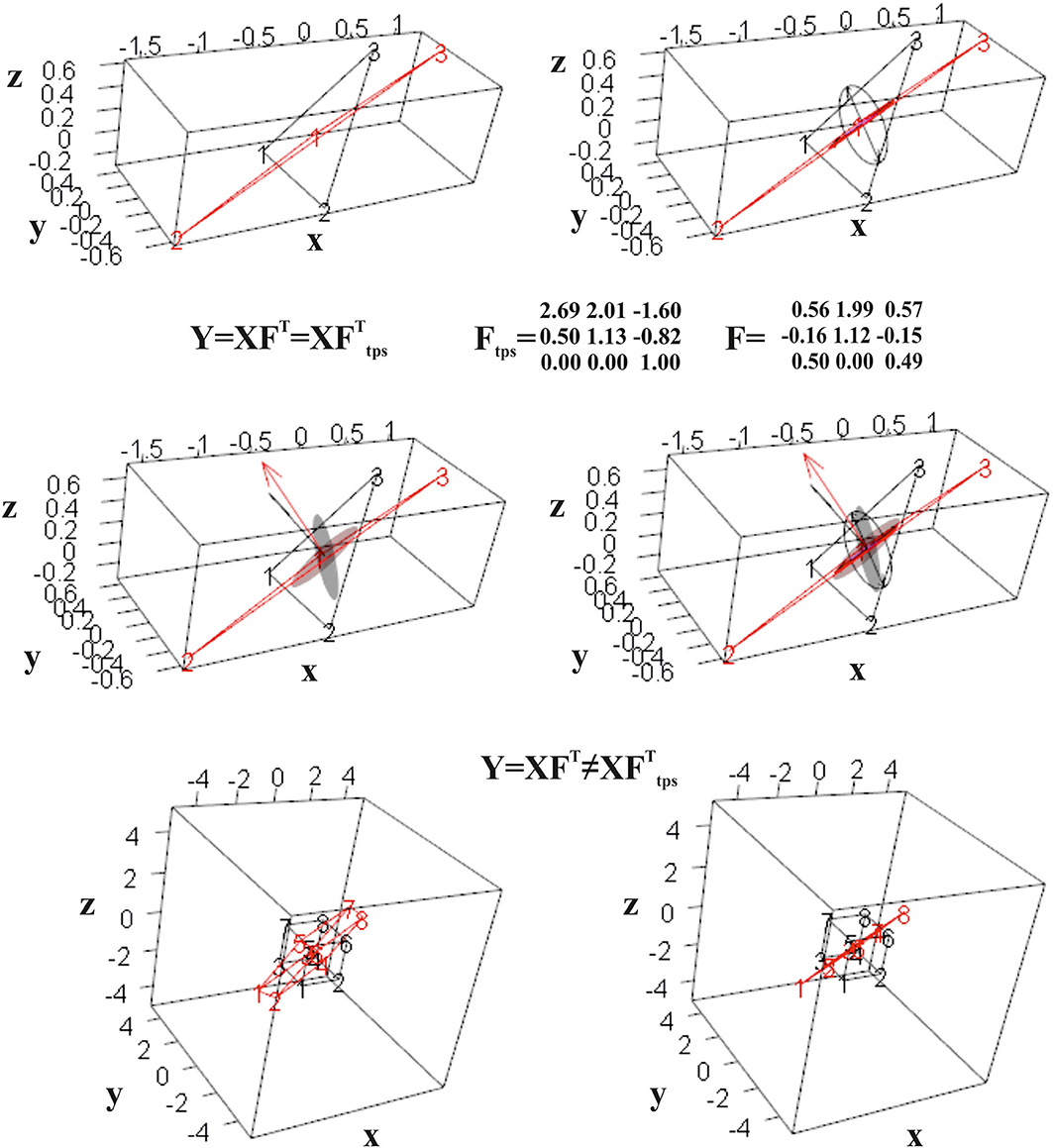
Figure 7. Computation of F for two triangles in ℝ3. Top row: the undeformed black triangle is deformed into the red one; the direct computation leads to a tensor that flattens a unitary sphere in an ellipse in ℝ3. Mid row: Ftps deforms a unitary sphere into an ellipsoid. Both F and Ftps return the deformed state if used to deform the source triangle. Bottom row: when applied to a regular cube, only F deforms it into a flat shape, while it does not hold for Ftps.
It is worth noticing that if X and Y are two coplanar triangles w.r.t. each other but still in ℝ3, the direct calculation still returns F and C while TPS cannot find a solution as the L matrix (Bookstein, 1989) becomes singular; it happens as in the absence of any displacement, between X and Y, along the dimension perpendicular to the plane containing them, no interpolation is possible in ℝ3.
The abovementioned example therefore suggests that, when looking at a surface's elements, deformation estimated by TPS could not be adequate to interpret what happens on them. Another simple example is to deform a cube with a known F and looking what happens to a single cube's faces. Figure 8 synthetically depicts this simple experiment. The ellipsoids at the cubes' centroids (source and target) were generated using and F, respectively. Using the direct discrete computation explained above, and , e.g., the projections of F and C on the faces, were calculated for any face and corresponding deformation ellipses were drawn. As it can be seen, these ellipses are very different descriptors w.r.t. the deformation encoded in the ellipsoid. on a specific face is just the projection of F on the plane containing the face. To project C, we calculate a1s and a2s on a face on the source shape X, as the vector differences between two vertices p1s and p2s and X centroid xc and their normal vector
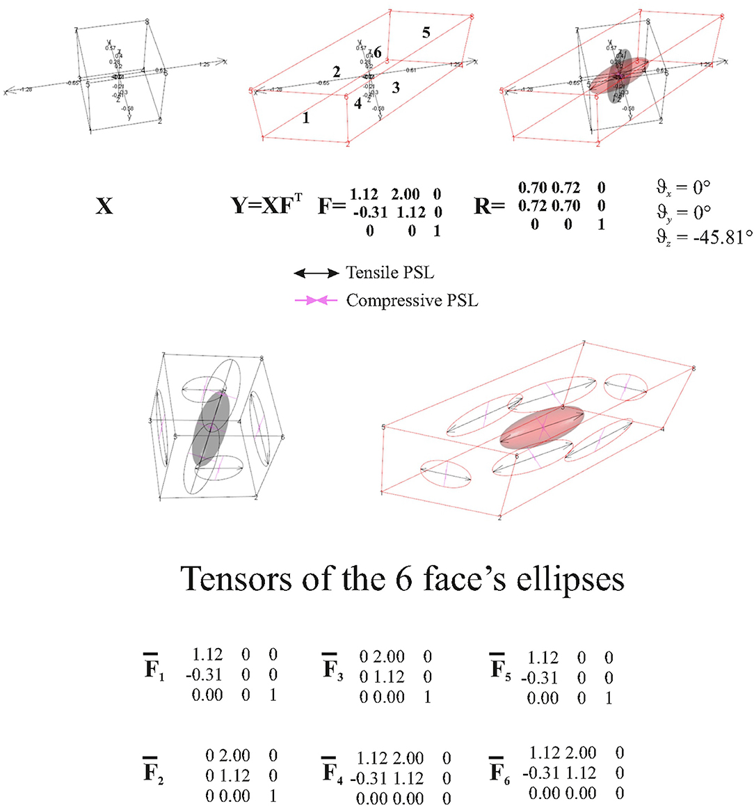
Figure 8. Top row: a regular black cube is deformed onto the red parallelepiped. Bottom row: F is then projected onto single faces using the procedure exposed in the text. Six projected tensors are then obtained.
The normalized axis perpendicular to a1s and a2s is found as
The projector on the source Ps is derived as
is then found as
we derived Pt (in the same way used for deriving Ps); then, can be found using
This procedure can be done for any face for which or need to be calculated.
Examples
Simulated Example
Figure 9 shows a regular square grid composed of 49 landmarks that is deformed in an irregular shape that is stretched and compressed in two different landmark columns, respectively. The procedure for estimating an approximately homologous triangulation as explained above on both source and target is also shown. The deformed shape is rotated onto the undeformed one via OPA without scaling. Figure 10 shows the first options we present for the visualization of local deformation. 2 × 2 local tensors (F for the target and for the source) have been used to deform unitary circumferences appropriately rescaled (magnification: 0.07). The color of each ellipse corresponds to the log(det(F)), thus indicating the local infinitesimal area ratio between target and source. Values < 0 indicate a reduction in local areas, values > 0 denote an enlargement, while 0 indicates no area change. The change in area alone does not inform about the direction of the deformation given by SD. Here, they are black if tensile and violet if compressive. In this example, all SD1 are tensile and they are larger in correspondence of the two columns of landmarks that undergo a compression and an expansion, respectively. We also depicted SD without ellipses; this gives a more clear perception of the direction and magnitude of local deformation only. The effect of rotation encoded in F is highly visible when using F on target or on source shape.
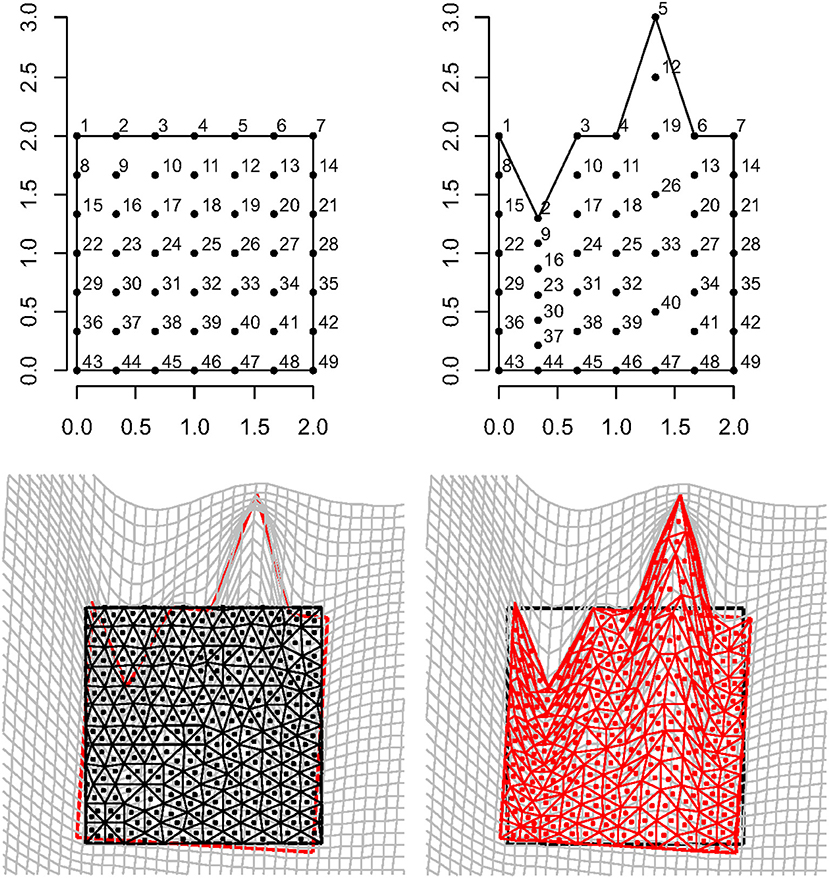
Figure 9. Top row: a regular square grid (left) is deformed onto an irregular polygon (right). Bottom row: a constrained Delaunay triangulation derived on the source shape (left) is estimated on the target using TPS; source and target shapes were aligned via OPA. Triangle's centroids will be used as evaluation points for estimating F, ∇∇(ψ), and other metrics.
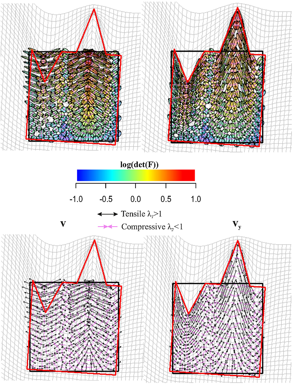
Figure 10. Top row: C (left) is used to deform unitary spheres appropriately rescaled for sake of visualization; F (right) was used for the same purpose on the target configuration. Ellipse's color is proportional to log(det(F)). Values < 0 indicate a reduction in local area, values > 0 indicate an expansion. Bottom row: the direction of deformation is dictated by vy and (i.e., SD = ellipse's axes). Tensile and compressive SD actions are indicated. Source and target shapes were aligned via OPA.
Figure 11 shows in the upper left panel the interpolation (via TPS) within the entire body of log(det(F)), while in the upper right panel, log(φ) density interpolated in the same manner. Larger values, as expected, can be found around regions corresponding to the two landmark's columns subjected to stretching and compression. In the lower left panel, we show the distribution of (||ΔΔ(ψ)n||2) density: here, we can appreciate the “non-affinity” of deformation around points where ∇∇(ψ) was evaluated; (||ΔΔ(ψ)n||2) density is distributed on alternate bands of large and small values with largest values in correspondence of the two landmark's columns that were stretched and compressed.
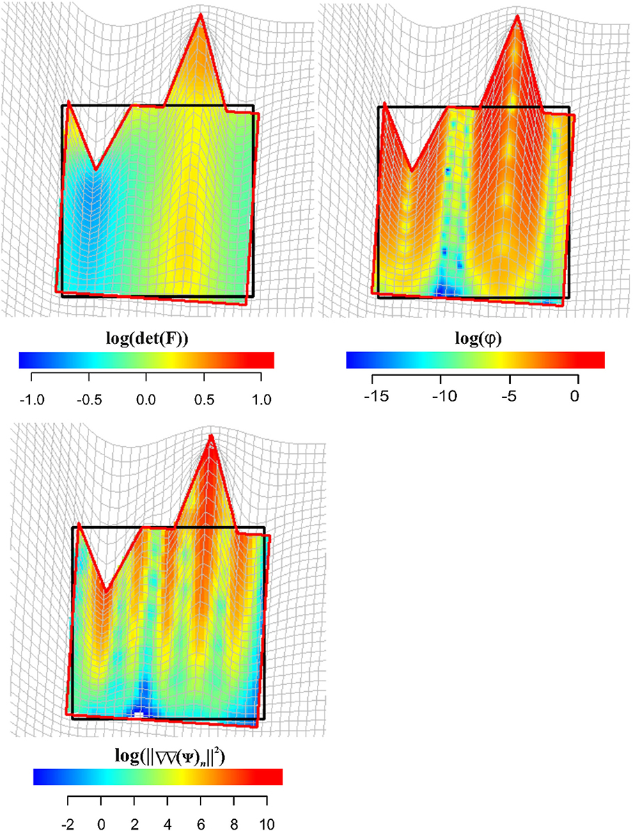
Figure 11. Visualization of local deformation via interpolation (using TPS) of log(det(F)), log(ϕ), and . Source and target shapes were aligned via OPA.
Real Examples
2D Paleontological Case Study
The 2D real example is related to the deformation occurring between two configurations in lateral view of two Hippopotamidae species: the extinct species Archaeopotamus harvardi from the Late Miocene of Eastern Africa (Coryndon, 1977; Harrison, 1997; Boisserie, 2005), here considered as the undeformed shape, and the extant species Hippopotamus amphibius distributed on the sub-Saharan African continent (Lewison and Pluháček, 2017) treated as the target shape. A. harvardi is one of the most primitive species within Hippopotamidae and displays some peculiar plesiomorphic traits including the low orbits whose rim flushes not beyond the profile of cranial roof. Moreover, the skull is shorter and less massive than in the extant hippo, with lower orbits and a slender zygomatic arch. The latter features are also present in the pigmy-insular Madagascan hippos (Pandolfi et al., 2020), which are characterized by reduction of size with respect to their continental ancestors, by a general decrease of the height of the orbits (Caloi and Palombo, 1994), and by brain size reduction (Weston and Lister, 2009). The opposite condition can be found in more derived Hexaprotodon (H. palaeindicus) and in H. amphibius (Boisserie, 2005, 2007; Boisserie et al., 2011; Pandolfi et al., 2020): in these species, orbits are elevated beyond the cranial roof. Elevated orbits, a long facial region, and a short postorbital part of the skull in Hippopotamidae are related to specialization for a semiaquatic lifestyle.
The adaptation to a semiaquatic lifestyle evolved independently in Hippopotamus and Hexaprotodon, suggesting a convergence between the two lineages (Boisserie, 2005, 2007; Boisserie et al., 2011 and references therein).
The morphological information encoded in Hippopotamidae skull lateral view is thus very important to depict evolutionary patterns during clade diversification, morphological convergences, and adaptations to different lifestyles including terrestrialization of some species (e.g., H. madagascariensis).
Figure 12 shows results relative to this 2D example.
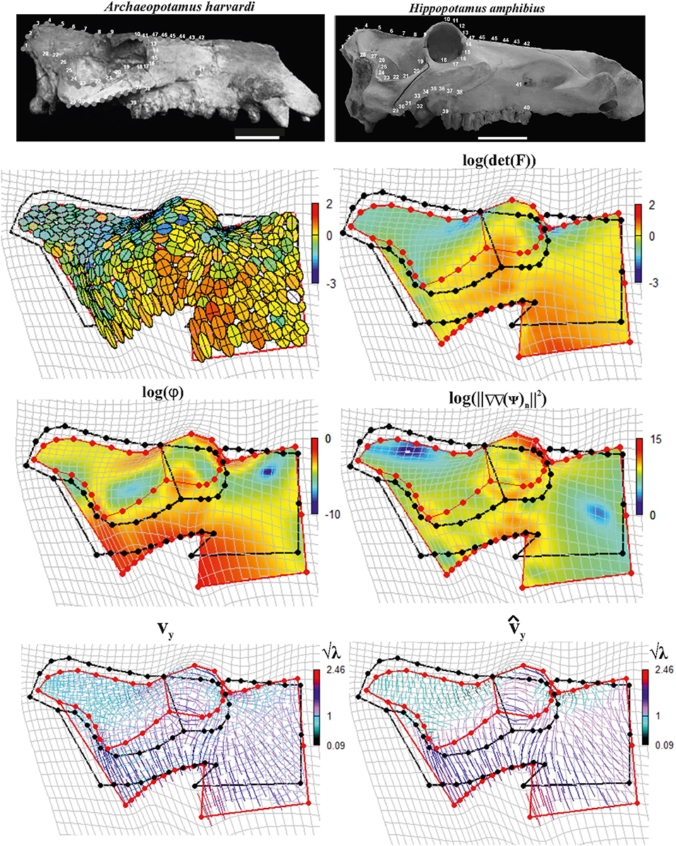
Figure 12. Local deformations observable between Archaeopotamus harvardi KNM-LT 4 (as source) and Hippopotamus amphibius MSNF 1135 (as target). We show both deformation ellipses obtained using F as well as main metrics derived using approaches explained in the text. In particular, we show log(det(F)), log(ϕ), and log(||∇∇(ψ)n ||2). vy and are also shown colored according to corresponding values in the interval ; values < 1 indicate compressive vy and , values > 1 indicate tensile actions. Source and target shapes were aligned via OPA. Scales equal 10 cm. KNM, Kenya National Museum; MSNFS, Museo di Storia Naturale di Firenze, sezione di Zoologia La Specola.
We digitized 15 landmarks and 32 semi-landmarks from photographs in lateral view on each specimen using the tpsDig2 v. 2.17 software (Rohlf, 2013). Semi-landmarks were used to capture the morphology of complex outlines where anatomical homology is difficult to recognize. See Figure 1 in Pandolfi et al. (2020) for landmarks definition. Semi-landmarks assume that curves or contours are homologous among specimens (Adams et al., 2004; Perez et al., 2006). First, a GPA implemented in the procSym() function from the R-package “Morpho” (Schlager, 2014) was used to rotate, translate, and scale landmark configurations to unit CS; here, we used the minimization of bending energy during the sliding of semi-landmarks as an alignment method. Second, OPA was used to align the two configurations. During OPA, the semi-landmarks previously used to align shapes with their consensus were treated as fixed landmarks, an approximation here considered not relevant for the purposes of the present article. The second row in Figure 12 shows the direction of SD and deformed ellipses (left side) colored according to log(det(F)), while on the right side, log(det(F)) has been continuously interpolated (using TPS) on the body domain of the target shape. The third row shows on the left side log(φ) and log(||ΔΔ(ψ)n||2) densities (right side), respectively. The fourth row shows SD on the left side and PSD on the right side. SD and PSD are colored according to and , respectively.
From all these panels, an interesting pattern emerges: the elevated orbit of H. amphibius has, on its upper borders, approximately horizontal PSD as also visible by oblique/horizontal ellipses in the second row (left) of Figure 12. This means that the “elevation” of the orbit and related structures takes place on the ventral side of the skull in lateral view; in fact, this is observable on the PSD panel where it appears evident that PSDs are oriented vertically with in particular in the jugal area. Closely outside the orbit, instead, we find oblique/vertical PSD with indicating that, there, the target bones (the frontal and parietal in particular) experience a local dorso-ventral contraction.
Without the help of PSD, one could still look at the usual deformation grid, but it does not furnish equally clear details and, more importantly, cannot quantify locally the amount and direction of local deformation.
3D Paleontological Case Study
The first 3D example considers the deformation occurring between the humeral morphology of two Talpoidea species: the extinct Mesoscalops montanensis (Barnosky, 1981) from the Early Miocene of North America and the extant Neurotrichus gibbsii Baird 1858 distributed in northwestern United States and southwestern British Columbia. These two species belong to a clade (Talpoidea) well-known for including several fossorial moles (Piras et al., 2012, 2015). Among these species, different degrees of fossoriality can be found from complex tunnel diggers to more ambulatorial species. Fossoriality degree is linked mainly to the adaptation shown by humeral morphology. While slender humeri are less adapted to borrowing activity, the humeral morphology of subterranean species experienced several shape changes in both distal and proximal regions with evident enlargements in medio-lateral direction. Proscalopidae, the clade to which Mesoscalops belongs, shows one of the most peculiar humeral morphologies among mammals, with unique shape and mechanical stress in the context of burrowing species (Barnosky, 1981, 1982; Piras et al., 2015). For our experiment here, we used CT scan data from Piras et al. (2015) for M. montanensis and for the non-complex tunnel digger N. gibbsii. As our procedure requires homologous triangulation, we used the TPS coefficients found when applying TPS to the 32 landmarks set used in Piras et al. (2015) belonging to M. montanensis (as source) and to N. gibbsii (as target) to deform M. montanensis mesh; this allows dealing with meshes constituted by homologous landmarks and triangulations. In this example, when aligning source and target via OPA, we did not scale shapes at unit size in order to show the effect of size and shape variation when evaluated on a local triangle's surfaces on the whole ℝ3.
Figure 13 shows data and results relative to this analysis. Triangle face colors correspond to log(det()), while (i.e., PSD plotted on the target) color is proportional to computed either on C or on , i.e., on tensors evaluated at the triangle's centroids on the whole ℝ3 (Figure 13, third row, right) or successively projected on the triangle's surfaces (Figure 13, third row, left). Corresponding distributions of these metrics are also illustrated. log(det()) presents all values < 0, thus indicating a considerably smaller size of target shape as exemplified by source shaded silhouette. and computed upon C or and F or respectively, give different information: in fact when using C and F, we obtain centripetal PSD dictated by size change with constantly < 0, while using and we observe PSDs that are formally tangent to the body surface but with that in some cases have values >1, thus indicating an expansion. We note here that it is not inherently better looking at or F. We highlight that, in most cases, this distinction is not considered and very often only deformation on meshes' surface is described and interpreted in functional, morphological, or biomechanical terms. This could lead to an incomplete or partial appreciation of the actual deformative phenomenon under study. This ineffectiveness could be partially mitigated by performing analyses in the shape-space. We used here the size-and shape-space with a purely didactic aim as it makes more evident the fact that PSDs of the whole body (thus not the body surface) when the target is considerably smaller than the source are very different from those on its surface.
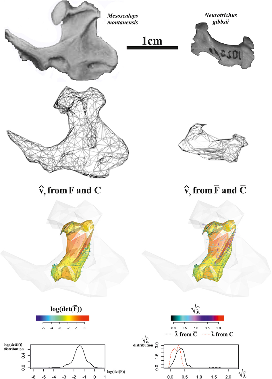
Figure 13. Local deformations observable between Mesoscalops montanensis UWBM 54708 (as source) and Neurotrichus gibbsii LACM 093944 (as target). 3D meshes are also shown. calculated upon F or are shown and colored according to the corresponding . Meshes' triangular faces are colored according to log(det()). Densities of relevant metrics are also illustrated. Source and target shapes were aligned via OPA without scaling. UWBM, University of Washington, Burke Memorial Washington State Museum, Seattle; LACM, Los Angeles County Museum.
Surfaces in 3D
The 3D surface example observes the occipital scale (exocranial surface) of two Homo erectus skulls from Java: Trinil 2 skull (belonging to the original Dubois collection from 1891's excavation) is of uncertain age, the estimate spanning from about 1 Ma and 0.5 Ma, and Ngandong 12 from Ngandong site (discovered in 1933 by von Koenigswald) about 50 km north from Trinil dated between 550 and 143 ka by Indriati et al. (2011) and recently re-placed between 110 and 120 ka by Rizal et al. (2020).
We digitized 133 landmarks distributed over the entire bone surface between the superior nuchal lines and the lambda on Ngandong 12 CT scans kindly provided by Dominique Grimaud-Hervé (GE medical systems/high speed RP; voxel size: 512 × 512 pixels; pixel size: 0.48; slice increment: 1 mm) and on Trinil 2 acquired with NextEngine laser scanner at the Department of Environmental Biology (Sapienza University of Rome). The configurations of points were digitized through the 3D software EVAN Toolbox v. 1.0 (www.evan-society.org). The same software was used for the 3D sliding procedure. In this way, 129 semi-landmarks were defined in relation to 4 fixed landmarks represented by the lambda, the inion and the two asterions (left and right). Spline relaxation (Bookstein, 1996, 1997) was carried out by sliding semi-landmarks on a plane tangent to the surface of each specimen (Gunz et al., 2005). This procedure involves the minimization of the bending energy with respect to the distribution of semi-landmarks on the surface of the three-dimensional object (not on a single curve) with reference to the position of the selected fixed landmarks and ensures the geometric homology (Gunz et al., 2005) of the points between the configurations. Configurations were then symmetrized w.r.t. sagittal plane.
The target was aligned to the source via OPA and both shapes were scaled at unit CS. For the sake of visualization, we decimated triangulation of meshes in order to better show deformation ellipsoids (see below). Figure 14 shows data collection and results relative to computation of F, and related metrics. Trinil 2 and Ngandong 12 are usually ascribed to the same species, i.e., H. erectus, albeit Trinil 2 is commonly considered a more primitive stage in H. erectus evolution, while Ngandong 12 constitutes, probably, a more derived form. Ngandong 12 shows a larger encephalization than Trinil 2 with a more elevated occipital scale relatively to the lambda. However, in both specimens, the opistocranion (the most distant point from the glabella) coincides with inion. A very marked difference is the morphology of occipital torus that is approximately straight in Trinil 2, while in Ngandong 12, it is a jutting structure laterally arching and with a noticeable thickness both medially and laterally. The orientation of varies considerably if they are computed upon F or . We depicted the ellipsoids circumscribed to computed from F: they clearly cross the body surface and are oriented in some regions nearly orthogonally to computed upon . This detail deserves particular attention as, looking at the surface only, one would underestimate the fact that the deformation acts primarily along a direction that, in some regions, is far from being tangent to the surface itself. In particular, the dorsal region of occipital scale, which includes the lambda, is more elevated dorso-ventrally in Ngandong 12 than in Trinil 2. This is related to the more pronounced dorso-ventral flattening of the latter w.r.t. the former that presents also a larger cranial capacity. Lack of cultural evidences, such as particular lithic industry, does not allow linking the larger encephalization of Ngandong 12 with an increased complexity of cultural behavior. Instead, the shape of occipital scales was probably more related to the development of neck muscles expansion and the antero-posterior deformation indicated by computed from F (and much less clearly by ) can be interpreted just as the structural bone response to nuchal muscle hyper-development. We suggest that the use of F instead of leads to a very different morphological reading of the actual local deformation process than looking at surfaces only. The OPA (or GPA) alignment, in fact, superimposes centroid's shapes and globally rotates them in such a way that the target could appear less deformed locally than it does actually. Local strain analysis, instead, being locally rotation-independent, allows visualizing and quantifying PSDs and their magnitudes independently from initial position of source and target.
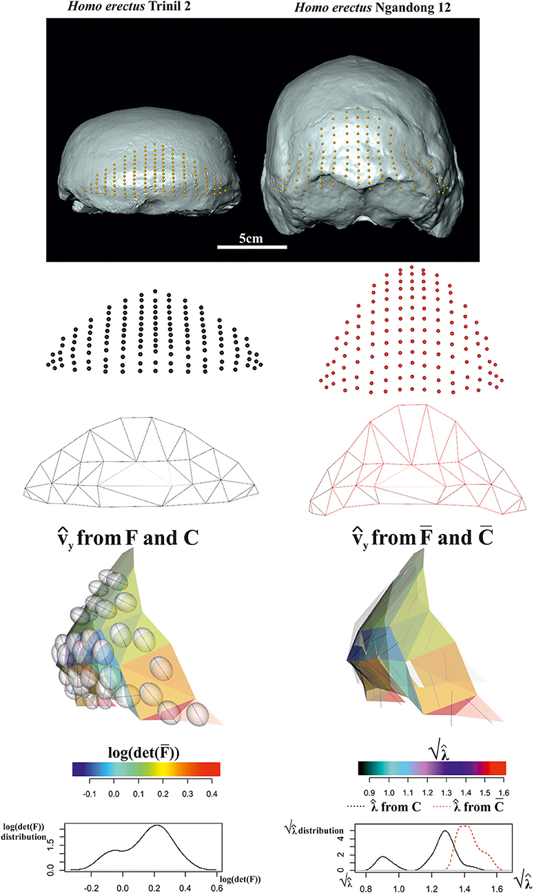
Figure 14. Local deformations observable between Homo erectus Trinil 2 (as source) and H. erectus Ngandong 12 (as target). 3D meshes are also shown. calculated upon F or are shown and colored according to the corresponding . Meshes' triangular faces are colored according to log(det()). Densities of relevant metrics are also illustrated. Source and target shapes were aligned via OPA. Trinil 2 is housed at the Nationaal Museum van Natuurlijke Historie, Leiden, The Netherlands; Ngandong 12 is housed at the Department of Physical Anthropology, Gadja Mada University College of Medicine, Yogyakarta, Indonesia.
Discussion and Conclusions
In this study, we presented several strategies in order to quantify and visualize local deformation in the context of geometric morphometrics, a kind of shape analysis that exploits the concept of homologous landmarks digitization. Starting from corresponding points found on both the source and target shapes, reasonably homologous triangulations can be assembled using constrained Delaunay triangulation (or similar strategies) on both two and three dimensions. Table 1 presents the main objects, together with their definitions, presented in the text. The use of direct calculation on triangles (or tetrahedra if available) or of the evaluation of ∇(ψ) at appropriate evaluation points leads to the identification of the deformation gradient tensor F that is the base to derive the necessary objects needed for the quantification of local deformation and for its visualization on source or target shape: C = FTF, v, and λ, i.e., the eigenvectors and eigenvalues of C; log(det(F)) has been used in the past (Márquez et al., 2012) to illustrate the infinitesimal area change around the evaluation points. However, this does not inform about the direction of deformation. SDs, e.g., v and vy, are proper objects for this purpose: they notify the (locally affine) directions of deformation dictated by C and F and can be further investigated by selecting PSDs, i.e., the primary direction of local shape change corresponding to those eigenvalues most distant from 1 (that indicates no deformation). We have shown that depicting SD could be very effective for interpreting the shape change and allows identifying particular regions characterized by deformations whose effects take place in different parts of the target shape as illustrated in the 2D example regarding orbit elevation in Archaeopotamus and Hippopotamus. In three dimensions we distinguished the two cases of “full volume” shapes, such as in Talpoidea example, and “shell-like” configurations such as in H. erectus occipital scale example. In these cases, we highlighted the importance of interpreting F or : in fact, looking at what happens to a triangle's surface cannot account for the deformation of the entire ambient space that also embraces the landmarks belonging to the surface itself. F, in fact, models deformation in every space direction and allows the appreciation of actual PSD representing the full shape change between source and target. Of course, both F and can be used to interpret the phenomenon. It is important, however, to be aware of what really means, i.e., a projection of the local actual deformation in three dimensions. While, in most GM applications related to paleontological and biological studies, the evaluation of local deformation in a quasi-continuous way is not very common, it could be of great help in inferring the deformational phenomenon when referred to bone's growth and development: for example, appreciating concomitantly ∇(ψ) and ∇∇(ψ) would permit the evaluation of the direction at specific locations of developmental process as well as its local variation possibly related to specific growth factors: in fact, as the growth is not an isotropic process (i.e., not homothetic), observing the eigendecomposition and spatial variation of the gradient tensor would inform about differential forces involved in the whole system. These forces could be related to muscle insertions such as in long bones of sauropod dinosaurs (Bonnan, 2007) or to mechanical pressures exerted in the complex reciprocal relationships existing between brain and its braincase abundantly investigated in paleoanthropology (Bruner, 2018). The range of use of the methods presented here is as wide as the range of shape analysis applications; their implementation is now available in R language using a set of specific ad hoc functions available in the online Supplementary Material together with scripts to reproduce each figure of the present paper. Each script is intended to work “stand alone” after loading the source file with ancillary functions and necessary R packages indicated therein. No workspace loading is necessary and landmark coordinates are furnished in individual scripts. More indications can be found in the “read me” file.
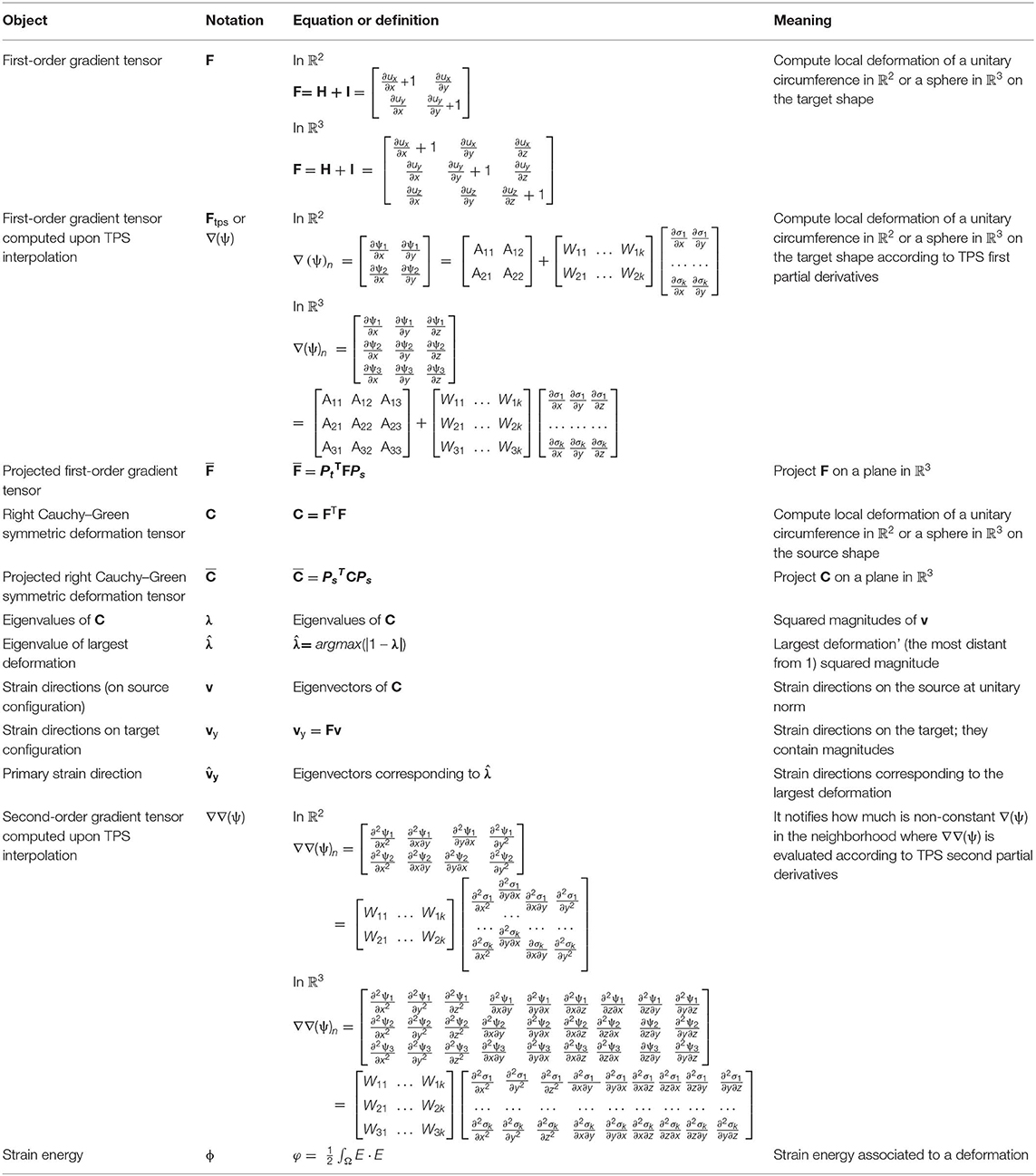
Table 1. Relevant objects used for visualization of local deformation.
Data Availability Statement
All the data used in this study can be generated by running the R scripts associated to the article.
Author Contributions
PP and VV conceived the paper. PP, PR, AM, and LP wrote the paper. AP, LP, and FD acquired experimental data. PP, VV, and SC implemented necessary R functions.
Conflict of Interest
The authors declare that the research was conducted in the absence of any commercial or financial relationships that could be construed as a potential conflict of interest.
Acknowledgments
We thank Luciano Teresi for useful advice during manuscript preparation. LP developed part of this paper within the research project Ecomorphology of fossil and extant Hippopotamids and Rhinocerotids granted by the University of Florence (Progetto Giovani Ricercatori Protagonisti initiative). We also thank two reviewers for useful suggestions during manuscript preparation.
Supplementary Material
The Supplementary Material for this article can be found online at: https://www.frontiersin.org/articles/10.3389/feart.2020.00066/full#supplementary-material
References
Adams, D. C., Rohlf, F. J., and Slice, D. E. (2004). Geometric morphometrics: ten years of progress following the ‘revolution'. It. J. Zool. 71, 5–16. doi: 10.1080/11250000409356545
Adams, D. C., Rohlf, F. J., and Slice, D. E. (2013). A field comes of age: geometric morphometrics in the 21st century. Hystrix, Ital. J. Mammal. 24, 7–14.
Angulo-Bedoya, M., Correa, S., and Benítez, H. A. (2019). Unveiling the cryptic morphology and ontogeny of the Colombian Caiman crocodilus: a geometric morphometric approach. Zoomorphology 138, 387–397. doi: 10.1007/s00435-019-00448-2
Barnosky, A. D. (1981). A skeleton of Mesoscalops (Mammalia, Insectivora) from the Miocene deep river formation, montana, and a review of the proscalopid moles: evolutionary, functional, and stratigraphic relationships. J. Vert. Pal. 1, 285–339. doi: 10.1080/02724634.1981.10011904
Barnosky, A. D. (1982). Locomotion in moles (Insectivora, Proscalopidae) from the middle Tertiary of North America. Science 216, 183–185. doi: 10.1126/science.216.4542.183
Boisserie, J. R. (2005). The phylogeny and taxonomy of Hippopotamidae (Mammalia: Artiodactyla): a review based on morphology and cladistic analysis. Zool. J. Linn. Soc. 143, 1–26. doi: 10.1111/j.1096-3642.2004.00138.x
Boisserie, J. R. (2007). “Family hippopotamidae,” in The Evolution of Artiodactyls, eds D. R. Prothero and S. E. Foss (Baltimore, MD: JHU Press), 106–119.
Boisserie, J. R., Fisher, R. E., Lihoreau, F., and Weston, E. M. (2011). Evolving between land and water: key questions on the emergence and history of the Hippopotamidae (Hippopotamoidea, Cetancodonta, Cetartiodactyla). Biol. Rev. 86, 601–625. doi: 10.1111/j.1469-185X.2010.00162.x
Bonnan, M. F. (2007). Linear and geometric morphometric analysis of long bone scaling patterns in Jurassic neosauropod dinosaurs: their functional and paleobiological implications. Anat. Rec. 290, 1089–1111. doi: 10.1002/ar.20578
Bookstein, F. L. (1989). Principal warps: thin-plate splines and the decomposition of deformations. IEEE Trans. Pattern Anal. Mach. Intell. 11, 567–585. doi: 10.1109/34.24792
Bookstein, F. L. (1991). Morphometric Tools for Landmark Data: Geometry and Biology. Cambridge: Cambridge University Press.
Bookstein, F. L. (1996). “Standard formula for the uniform shape component in landmark data,” in Advances in Morphometrics, eds L. F. Marcus, M. Corti, A. Loy, G. J. P. Naylor, and D. E. Slice (Boston, MA: NATO ASI Series; Series A; Life Sciences; Springer), 153–168.
Bookstein, F. L. (1997). Landmark methods for forms without landmarks: morphometrics of group differences in outline shape. Med. Im. An.1, 225–243. doi: 10.1016/s1361-8415(97)85012-8
Bruner, E. (2018). “The brain, the braincase, and the morphospace,” in Digital Endocasts, eds E. Bruner, N. Ogihara, and H. C. Tanabe (Tokio: Springer), 93–114.
Caloi, L., and Palombo, M. R. (1994). Le faune a grandi mammiferi del Pleistocene superiore dell'Italia centrale: biostratigrafia e paleoambiente. Boll. Serv. Geol. Ital. 111, 503–514.
Castiglione, S., Serio, C., Tamagnini, D., Melchionna, M., Mondanaro, A., Di Febbraro, M., et al. (2019). A new, fast method to search for morphological convergence with shape data. PLoS ONE 14:e0226949. doi: 10.1371/journal.pone.0226949
Ceritoglu, C., Tang, X., Chow, M., Hadjiabadi, D., Shah, D., Brown, T., et al. (2013). Computational analysis of LDDMM for brain mapping. Front. Neurosci. 7:151. doi: 10.3389/fnins.2013.00151
Charlier, B., Charon, N., and Trouvé, A. (2017). The fshape framework for the variability analysis of functional shapes. Found. Comput. Math. 17, 287–357. doi: 10.1007/s10208-015-9288-2
Colangelo, P., Ventura, D., Piras, P., Pagani Guazzugli Bonaiuti, J., and Ardizzone, G. (2019). Are developmental shifts the main driver of phenotypic evolution in Diplodus spp. (Perciformes: Sparidae)? BMC Evol. Biol. 19:106. doi: 10.1186/s12862-019-1424-1
Coryndon, S. C. (1977). The taxonomy and nomenclature of the Hippopotamidae (Mammalia, Artiodactyla) and a description of two new fossils species. Proc. Kon. Ned. Akad. Wetensch. B. 80, 61–88.
Dryden, I. L., and Mardia, K. V. (2016). Statistical Shape Analysis, With Applications in R, 2nd Edn. Chichester: John Wiley and Sons.
Durrleman, S., Pennec, X., Trouvé, A., Ayache, N., and Braga, J. (2012). Comparison of the endocranial ontogenies between chimpanzees and bonobos via temporal regression and spatiotemporal registration. J. Hum. Evol. 62, 74–88.
Evangelista, A., Gabriele, S., Nardinocchi, P., Piras, P., Puddu, P. E., Teresi, L., et al. (2015). “Continuum mechanics meets echocardiographic imaging: investigation on the principal strain lines in human left ventricle,” in Developments in Medical Image Processing and Computational Vision, eds J. Tavares and J. R. M. Natal (Cham: Springer), 41–54.
Gabriele, S., Teresi, L., Varano, V., Nardinocchi, P., Piras, P., Esposito, G., et al. (2016). “Mechanics-based analysis of the left atrium via echocardiographic imaging,” in Proceedings of the 5th Eccomas Thematic Conference on Computational Vision and Medical Image Processing, eds J. Tavares and J. R. M. Natal (Boca Raton, FL: VipIMAGE 2015, CRC press), 267–271.
Gower, J. C. (1975). Generalized procrustes analysis. Psychometrika 40, 33–51. doi: 10.1007/BF02291478
Gunz, P., Mitteroecker, P., and Bookstein, F. L. (2005). “Semilandmarks in three dimensions,” in Modern Morphometrics in Physical Anthropology, ed D. E. Slice (Boston, MA: Springer), 73–98.
Harrison, T. (1997). “The anatomy, paleobiology, and phylogenetic relationships of the Hippopotamidae (Mammalia, Artiodactyla) from the Manonga Valley, Tanzania,” in Neogene Paleontology of the Manonga Valley, Tanzania, ed T. Harrison (Boston, MA: Springer), 137–190.
Indriati, E., Swisher, C. C., Lepre, C., Quinn, R. L., Suriyanto, R. A., Hascaryo, A. T., et al. (2011). The age of the 20 meter Solo River terrace, Java, Indonesia and the survival of Homo erectus in Asia. PLoS ONE 6:e21562. doi: 10.1371/journal.pone.0021562
Kent, J. T., and Mardia, K. V. (1994). “The link between kriging and thin-plate splines,” in Probability, Statistics and Optimization: A Tribute to Peter Whittle, ed F. P. Kelly (New York, NY: Wiley), 325–39.
Kratz, A., Auer, C., Stommel, M., and Hotz, I. (2013) Visualization analysis of second-order tensors: moving beyond the symmetric positive-definite case. Comp. Graph. For. 32, 49–74. doi: 10.1111/j.1467-8659.2012.03231.x
Le, H.-L. (1988). Shape theory in flat and curved spaces and shape densities with uniform generators (Ph.D. dissertation). University Cambridge, Cambridge, United Kingdom.
Lewison, R., and Pluháček, J. (2017). Hippopotamus amphibius. IUCN Red List Threat. Species 2017:e.T10103A18567364. doi: 10.2305/IUCN.UK.2017-2.RLTS.T10103A18567364.en
Márquez, A., Moreno-González, A., Plaza, Á., and Suárez, J. P. (2014). There are simple and robust refinements (almost) as good as Delaunay. Math. Comp. Sim. 106, 84–94. doi: 10.1016/j.matcom.2012.06.001
Márquez, E. J., Cabeen, R., Woods, R. P., and Houle, D. (2012). The measurement of local variation in shape. Evol. Biol. 39, 419–439. doi: 10.1007/s11692-012-9159-6
Miller, M. I., Trouvé, A., and Younes, L. (2015). Hamiltonian systems and optimal control in computational anatomy: 100 years since D'Arcy Thompson. Annu. Rev. Biomed. Eng. 17, 447–509. doi: 10.1146/annurev-bioeng-071114-040601
Miller, M. I., Younes, L., and Trouvé, A. (2014). Diffeomorphometry and geodesic positioning systems for human anatomy. Technology 2, 36–43. doi: 10.1142/S2339547814500010
Oxnard, C., and O'Higgins, P. (2009). Biology clearly needs morphometrics. Does morphometrics need biology? Biol. Theory 4, 84–97. doi: 10.1162/biot.2009.4.1.84
Pandolfi, L., Martino, R., Rook, L., and Piras, P. (2020). Investigating ecological and phylogenetic constraints in Hippopotamidae skull shape. Riv. It. Paleont. Strat. 126, 37–49. doi: 10.13130/2039-4942/12730
Perez, S. I., Bernal, V., and Gonzalez, P. N. (2006). Differences between sliding semi-landmark methods in geometric morphometrics, with an application to human craniofacial and dental variation. J. Anat. 208, 769–784. doi: 10.1111/j.1469-7580.2006.00576.x
Piras, P., Buscalioni, A. D., Teresi, L., Raia, P., Sansalone, G., Kotsakis, T., et al. (2014). Morphological integration and functional modularity in the crocodilian skull. Int. Zool. 9, 498–516. doi: 10.1111/1749-4877.12062
Piras, P., Maiorino, L., Raia, P., Marcolini, F., Salvi, D., Vignoli, L., et al. (2010). Functional and phylogenetic constraints in Rhinocerotinae craniodental morphology. Evol. Ecol. Res. 12, 897–928.
Piras, P., Sansalone, G., Teresi, L., Kotsakis, T., Colangelo, P., and Loy, A. (2012). Testing convergent and parallel adaptations in talpids humeral mechanical performance by means of geometric morphometrics and finite element analysis. J. Morphol. 273, 696–711. doi: 10.1002/jmor.20015
Piras, P., Sansalone, G., Teresi, L., Moscato, M., Profico, A., Eng, R., et al. (2015). Digging adaptation in insectivorous subterranean eutherians. The enigma of Mesoscalops montanensis unveiled by geometric morphometrics and finite element analysis. J. Morphol. 276, 1157–1171. doi: 10.1002/jmor.20405
Piras, P., Torromeo, C., Evangelista, A., Esposito, G., Nardinocchi, P., Teresi, L., et al. (2019). Non-invasive prediction of genotype positive–phenotype negative in hypertrophic cardiomyopathy by 3D modern shape analysis. Exp. Physiol. 104, 1688–1700.
Piras, P., Torromeo, C., Evangelista, A., Gabriele, S., Esposito, G., Nardinocchi, P., et al. (2017). Homeostatic left heart integration and disintegration links atrio-ventricular covariation's dyshomeostasis in hypertrophic cardiomyopathy. Sci. Rep. 7, 1–12.
Rizal, Y., Westaway, K. E., Zaim, Y., van den Bergh, G. D., Bettis, E. A. III., Morwood, M. J., et al. (2020). Last appearance of Homo erectus at Ngandong, Java, 117,000–108,000 years ago. Nature 577, 381–385. doi: 10.1038/s41586-019-1863-2
Rohlf, F. J., and Bookstein, F. L. (2003). Computing the uniform component of shape variation. Syst. Biol. 52, 66–69. doi: 10.1080/10635150390132759
Rohlf, F. J., and Slice, D. (1990). Extensions of the Procrustes method for the optimal superimposition of landmarks. Syst. Biol. 39, 40–59. doi: 10.2307/2992207
Sansalone, G., Colangelo, P., Loy, A., Raia, P., Wroe, S., and Piras, P. (2019). Impact of transition to a subterranean lifestyle on morphological disparity and integration in talpid moles (Mammalia, Talpidae). BMC Evol. Biol. 19:179. doi: 10.1186/s12862-019-1506-0
Santos, B. F., Perrard, A., and Brady, S. G. (2019). Running in circles in phylomorphospace: host environment constrains morphological diversification in parasitic wasps. Proc. Royal Soc. B 286:20182352. doi: 10.1098/rspb.2018.2352
Schlager, S. (2014). Morpho: Calculations and Visualizations Related to Geometric Morphometrics. R-package version 2.0. 3–1.
Stayton, C. T. (2015). The definition, recognition, and interpretation of convergent evolution, and two new measures for quantifying and assessing the significance of convergence. Evolution 69, 2140–2153. doi: 10.1111/evo.12729
Trouvé, A. (1998). Diffeomorphisms groups and pattern matching in image analysis. Int. J. Comput. Vis. 28, 213–221.
Varano, V., Gabriele, S., Teresi, L., Dryden, I., Puddu, P. E., Torromeo, C., et al. (2017). The TPS direct transport: a new method for transporting deformations in the size-and-shape space. Int. J. Comp. Vis. 124, 384–408, doi: 10.1007/s11263-017-1031-9
Varano, V., Piras, P., Gabriele, S., Teresi, L., Nardinocchi, P., Dryden, I. L., et al. (2018). The decomposition of deformation: new metrics to enhance shape analysis in medical imaging. Med. Im. An. 46, 35–56. doi: 10.1016/j.media.2018.02.005
Varano, V., Piras, P., Gabriele, S., Teresi, L., Nardinocchi, P., Dryden, I. L., et al. (2019). Local and global energies for shape analysis in medical imaging. Int. J. Num. Meth. Biomed. Engin. 36:e3252. doi: 10.1002/cnm.3252
Weston, E. M., and Lister, A. (2009). Insular dwarfism in hippos and a model for brain size reduction in Homo floresiensis. Nature 459, 85–88. doi: 10.1038/nature07922
Keywords: local deformation, tensor visualization, strain directions, thin plate spline, first derivative, second derivative
Citation: Piras P, Profico A, Pandolfi L, Raia P, Di Vincenzo F, Mondanaro A, Castiglione S and Varano V (2020) Current Options for Visualization of Local Deformation in Modern Shape Analysis Applied to Paleobiological Case Studies. Front. Earth Sci. 8:66. doi: 10.3389/feart.2020.00066
Received: 15 November 2019; Accepted: 20 February 2020;
Published: 24 March 2020.
Edited by:
Paul Antony Selden, University of Kansas, United StatesReviewed by:
David A. T. Harper, Durham University, United KingdomManuel F. G. Weinkauf, Charles University, Czechia
Copyright © 2020 Piras, Profico, Pandolfi, Raia, Di Vincenzo, Mondanaro, Castiglione and Varano. This is an open-access article distributed under the terms of the Creative Commons Attribution License (CC BY). The use, distribution or reproduction in other forums is permitted, provided the original author(s) and the copyright owner(s) are credited and that the original publication in this journal is cited, in accordance with accepted academic practice. No use, distribution or reproduction is permitted which does not comply with these terms.
*Correspondence: Pasquale Raia, cGFzcXVhbGUucmFpYUB1bmluYS5pdA==
†These authors have contributed equally to this work