
94% of researchers rate our articles as excellent or good
Learn more about the work of our research integrity team to safeguard the quality of each article we publish.
Find out more
ORIGINAL RESEARCH article
Front. Earth Sci. , 11 December 2019
Sec. Cryospheric Sciences
Volume 7 - 2019 | https://doi.org/10.3389/feart.2019.00326
This article is part of the Research Topic Observational Assessments of Glacier Mass Changes at Regional and Global Level View all 12 articles
 Daniel Falaschi1,2*
 María Gabriela Lenzano1
 Ricardo Villalba1
 Tobias Bolch3
 Andrés Rivera4,5
 Andrés Lo Vecchio1,2
A full understanding of glacier changes in the Patagonian Andes over decadal to century time-scales is presently limited by a lack of detailed and appropriate long-term observations. Here, we present geodetic mass and area changes of three valley glaciers from Monte San Lorenzo derived from stereo aerial photos, the Shuttle Radar Topography Mission (SRTM) and satellite imagery (SPOT5 and Pleiades) spanning four periods from 1958 to 2018. Our results indicate that net mass balance was negative throughout the six decades, with a mean mass loss of −1.35 ± 0.08 m w.e. a–1 and a total glacier area loss of 14.2 ± 0.7 km2 (23 ± 1% or 0.40 ± 0.02% a–1). The period 1981–2000 had the most negative mass budget, with an area-averaged mass loss of 1.67 ± 0.11 m w.e. a–1 and a maximum loss of −2.23 ± 0.07 m w.e. a–1 at San Lorenzo Sur glacier. Over the periods of 2000–2012 and 2012–2018, the mass budget of these three glaciers remained virtually unchanged at −1.37 ± 0.06 and −1.36 ± 0.17 m w.e. a–1, respectively. To place these results into a broader geographical context, the mass balance of a further 15 glaciers from around the Monte San Lorenzo massif was determined from 2000 onwards. This wider analysis reveals a period of reduced mass loss of −0.13 ± 0.21 m w.e. a–1 from 2012 to 2018 after a period of enhanced mass loss of −0.31 ± 0.16 m w.e. a–1 between 2000 and 2012. We find that increasing air temperatures coupled with diminishing precipitation across the region explains the observed patterns and are the main drivers of the negative mass budget. Furthermore, increased calving and melting into recently formed proglacial lakes has further enhanced mass loss at some lake-terminating glaciers.
A sustained trend of rapid glacier retreat and depletion has been observed in most mountain and cold regions around the Globe (Zemp et al., 2019) including the Patagonian Andes (Davies and Glasser, 2012; Paul and Mölg, 2014; Masiokas et al., 2015; Falaschi et al., 2017; Dussaillant et al., 2019). The large, temperate ice masses of Patagonia are particularly sensitive to climate change as they are close to the melting point (Schwikowski et al., 2013), and are in fact currently among the greatest contributors to sea-level rise (Marzeion et al., 2012; Gardner et al., 2013; Foresta et al., 2018). In addition to glacier mass losses owed to climate change, the presence of glacial lakes at glacier terminus is known to boost glacier area reduction and glacier thinning through calving (Basnett et al., 2013; Brun et al., 2019). In the Patagonian Andes, proglacial lake expansion has been mostly observed in the large outlet glaciers flowing down the Patagonian Icefields (Harrison et al., 2006; Loriaux and Casassa, 2013), yet the influence of glacier-lake interactions in the shrinkage of smaller glaciers is poorly known.
Over the last five decades the investigation of glacier changes worldwide has been favored by the increased availability of systematically acquired satellite imagery and derived products such as digital elevation models (DEMs). Before the satellite era, glacier studies usually relied on aerial photographs (e.g., Corte and Espizúa, 1981; Espizúa, 1983; among others for the Andes). These, however, were most frequently not repeatedly acquired (see, e.g., Mölg et al., 2019), implied high operational costs, and were in principle hardly aimed at glaciological studies. Even more problematic, the acquisition geometry of air photographs resulted in the deformation of terrain features (e.g., glaciers), which is maximized in areas of mountain topography. This in turn made the use of specific hardware (a photo restitutor) and precise ground control points usually obtained during field surveys mandatory, resulting in a highly complex process. In some cases, glacier inventories were done without proper orthorectification of the aerial photographs (e.g., Bertone, 1960; Corte and Espizúa, 1981; Espizúa, 1983 in the Andes in particular), potentially introducing gross errors. In recent years, however, the advent of techniques such as Structure from Motion (SFM) has allowed for assessing glacier changes during the pre-satellite era without such demanding efforts (Mölg and Bolch, 2017; Vargo et al., 2017).
Whilst a number of recent studies have used declassified Corona and Hexagon imagery data to derive glacier changes in the 1960 and 1970s on several glacierised regions in the World (e.g., Bolch et al., 2008; Bhambri et al., 2011; Pieczonka and Bolch, 2015; Racoviteanu et al., 2015; Ragettli et al., 2016; Schmidt and Nüsser, 2017; Maurer et al., 2019; King et al., 2019), glaciological studies based on aerial photographs acquired in the mid 20th century are still scarce (e.g., Cox and March, 2004; Koblet et al., 2010; Pieczonka et al., 2011; Fieber et al., 2018; Farías-Barahona et al., 2019; Mölg et al., 2019).
In general terms, the understanding of glacier mass budget trends in southern Patagonia do not rely on long or numerous glaciological records. Quite the opposite, merely Martial Este (2001-ongoing; Strelin and Iturraspe, 2007; Buttstädt et al., 2009; see also WGMS, 2017) and Glaciar de los Tres (Popovnin et al., 1999, resumed in 2013 by the Instituto Argentino de Nivología y Glaciología of Argentina) have had glaciological mass balance programs recently. At a broader scale, glacier volume and mass changes been surveyed by means of the geodetic mass balance method (Rivera et al., 2007; Willis et al., 2012; Falaschi et al., 2017; Foresta et al., 2018; Braun et al., 2019; Dussaillant et al., 2019), which retrieves glacier elevation and volume changes by differencing a series of multi-temporal, often multi-sourced DEMs (Cogley, 2009). However, most of these mass balance assessments have utilized DEMs that represent the topography of glacier surface only from the year 2000 onwards (i.e., the Shuttle Radar Topography Mission, SRTM). Consequently, glacier mass changes during the earlier 20th century are hardly known. In very few cases, early 20th century DEMs have been produced by digitalization of contour maps (see Rignot et al., 2003), where uncertainties on height elevation are high.
In this study, we (1) produce a six decade (1958–2018) geodetic mass balance record for three valley glaciers in the Monte San Lorenzo massif (Río Oro, Río Lácteo, and San Lorenzo Sur), using a combination of multi-sourced DEMs (based on aerial photos, SRTM, SPOT 5, and Pleiades data) on a two-decadal to sub-decadal sale, providing this way the longest glacier mass balance record so far for the Patagonian Andes, (2) provide an updated 2000–2018 geodetic mass balance assessment for other 15 glaciers in the Monte San Lorenzo, (3) derive glacier area and length changes and (4) discuss the influence of climatic trends in the region and the formation and growth of proglacial lakes at glacier terminus that may help in giving an explanation to the observed glacier changes in the intervening years. Data presented in this paper will be made available in the WGMS and/or GLIMS database.
Monte San Lorenzo (47° 35′ S, 72° 18′ W, 3706 m a.s.l., Figure 1) is located in the southern Patagonian Andes, at the international border between Argentina (Santa Cruz Province) and Chile (Región de Aysén). On Argentinian territory, the massif lies within the San Lorenzo Conservation Area, and closely bounds with the Perito Moreno National Park. It is the second highest peak in Patagonia behind Monte San Valentín (3900 m a.s.l., Metzeltin Buscaini, 2005). Monte San Lorenzo forms, along with other lower mountain ranges, a heavily glaciated region in the eastern foreland of the Southern and Northern Patagonian Icefields (SPI and NPI, respectively). Wenzens (2002) showed that during the Last Glaciation in Patagonia, glaciers in the San Lorenzo area did not form a continuous ice cap encompassing also the SPI and NPI, and that glaciers in the eastern flank of Monte San Lorenzo drained eastwards independently from the icefields.
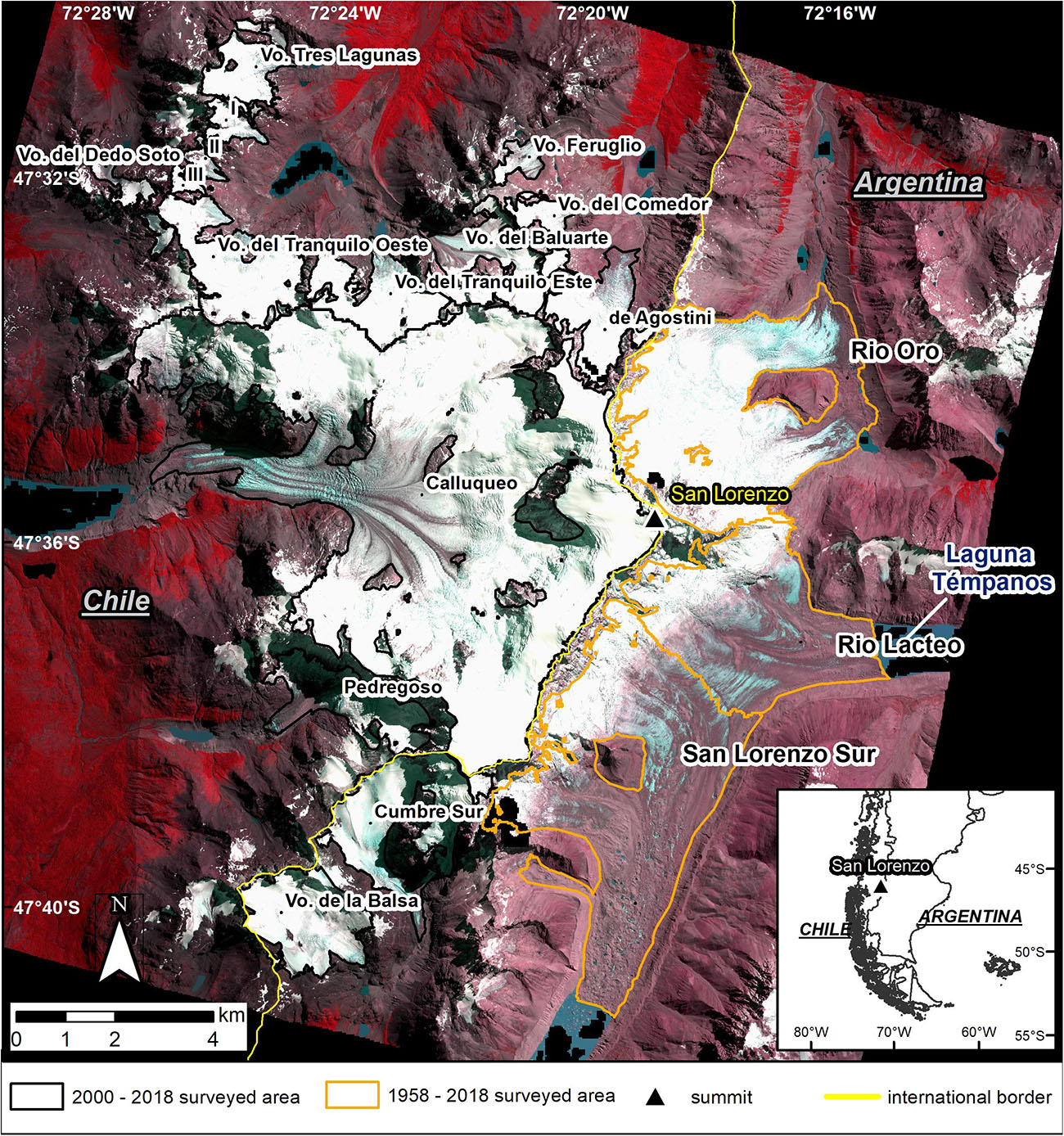
Figure 1. Overview of the Monte San Lorenzo area and the investigated glaciers. I, II and II stand for three unnamed glaciers in the Tres Lagunas basin. Background image is a Pleiades RGB 432 composition. Vo, Ventisquero (lower part of a glacier in Spanish).
From a glaciological perspective, Monte San Lorenzo was pivotal for establishing the chronology of glacier readvances since the Late-Glacial in southern Patagonia, since radiocarbon ages obtained at Río Lácteo glacier indicated that the onset of neoglaciations did not start until the Mid-Holocene (Mercer, 1968), much in agreement with the general scheme proposed by Aniya (2013). The work of Mercer (1968) was recently resumed by Morano-Büchner and Aravena (2013); Garibotti and Villalba (2017) and Sagredo et al. (2017), providing a detailed glacier fluctuation chronology of a number of Monte San Lorenzo glaciers based on lichenometry, surface exposure dating and historical photographic documents, from the Mid-Holocene through the Little Ace Age up to the year 1945. Falaschi et al. (2013) compiled the first glacier inventory of the Monte San Lorenzo and nearby peaks, accounting for ∼207 km2 ice in 2008, and estimated 1985–2008 glacier area reduction rates of ∼1% a–1, in agreement with the general trends observed elsewhere in Patagonia (Davies and Glasser, 2012; Paul and Mölg, 2014; Falaschi et al., 2017).
The abrupt, often intricate topography of Monte San Lorenzo results in a complex variety of cirque and valley glaciers with compound basins (Glasser and Jansson, 2008). The regenerated Río Lácteo and San Lorenzo Sur glaciers have a mostly debris-covered tongue that calve into proglacial lakes, whereas Río Oro is predominantly debris-free and has a land-terminating front (Falaschi et al., 2013). Accumulation Area Ratios (AAR) for these three glaciers are small (<0.5), which is indicative of glaciers in a disequilibrium state (Bakke and Nesje, 2011). The most reliable modern ELA determinations in the area stem from the nearby Río Tranquilo glacier at 1895 m a.s.l. (Sagredo et al., 2017).
Climate-wise, Monte San Lorenzo lies in a transitional maritime to continental area, within the strong West-East orographic precipitation gradient that characterizes the Patagonian Andes (Garreaud et al., 2013). Whilst the temperature variations are less pronounced across the main water divide (Wolff et al., 2013), the dissimilar environmental conditions result in diverse glacier thermal regimes and sensitivity to climate perturbations. Glaciers in the drier, eastern slope of the water divide (such as Río Oro, Río Lácteo and San Lorenzo Sur), may be polythermal and probably less sensitive to rising temperatures compared to the temperate glaciers on the wetter, western flank, where a decrease in the snow/rain ratio will have a greater impact on snow accumulation and thus on mass balance as well (Sagredo and Lowell, 2012).
In the historical aerial photography archive of the Instituto Geográfico Nacional of Argentina (IGN), there are few suitable photographs (no significant amounts of seasonal snow and cloud cover) for the years 1958 and 1981 (Table 1). These aerial photographs fully cover Río Oro, Río Lácteo and San Lorenzo Sur glaciers located in Argentinian territory (Figure 1). The 1958 and 1981 scenes were scanned from the negatives at 10 μm scanning resolution in a Vexcel UltraScan 5000 scanner.
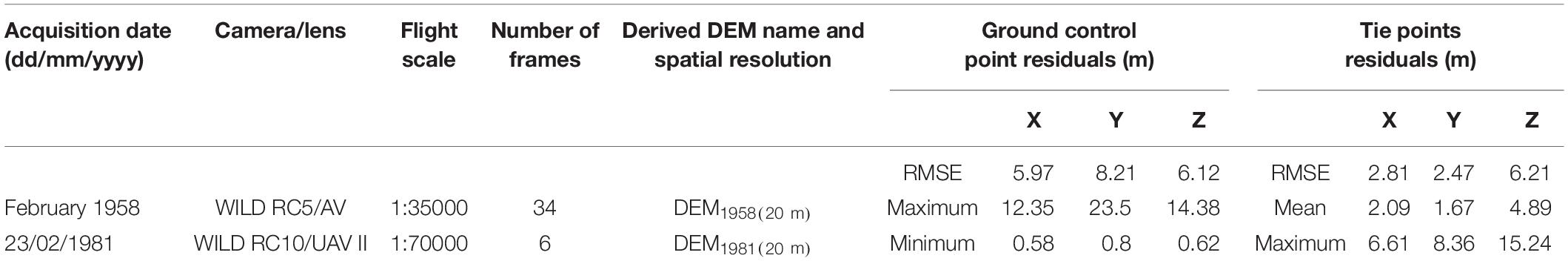
Table 1. Characteristics of the utilized aerial photos and derived DEMs.
The entire aerial photogrammetric processing, from the strip formation to DEM and orthophoto generation were carried out in the Photomod 4.1 software (Racurs, 2006). The basic workflow for DEM processing involves (1) block forming (2) aerial triangulation (3) block adjustment and (4) block processing. After arranging and orientating the images in strips during stage (1), block forming is used to perform interior orientation by flagging fiducial marks and relative orientation by measuring a total of 21 ground control points (Falaschi et al., 2017) on each frame. Additionally, tie points are placed within stereopairs according to the Von Gruber distribution (Kerner et al., 2016). Numerical adjustment of the model is accomplished in the block adjustment stage. A summary of ground control points and tie-point residuals after block adjustment are given in Table 1. Once the interior and external orientations are solved, any measured point will have xyz coordinates on the model.
Normally, final extraction of the photogrammetric DEM is carried out with automatic procedures, i.e., auto-correlation of homologous points on each stereopair in a photogrammetric software (Cox and March, 2004; Koblet et al., 2010). Instead of relying in automatisms, which will inevitably lead to outliers and data voids (Pieczonka et al., 2011), we materialized the DEMs by on-screen digitalization of breaklines (Lenzano, 2013) using LCD shutter stereoglasses. Breaklines represent natural terrain discontinuities such as mountain crests and valleys, slope changes, crevasses, lakes, or gullies. In general, the more complex the terrain, the denser placing of breaklines and breakline nodes will be. The area covered by the digitized breaklines covers the glaciers themselves but also part of the adjacent stable terrain, which serves for DEM coregistration and estimation of the uncertainty related to the glacier elevation changes (see section “Assessment of the Elevation Change Uncertainty”). Once the breaklines are finalized, they are converted to Triangular Irregular Networks (TINs) and ultimately DEMs are interpolated at 20 m resolution, considering the minor scale of the aerial photos (1:70.000, DEM1981 –see Table 1). Lastly, the original 1958 and 1981 aerial images are converted to orthofotos using the previously generated DEMs in the Photomod Mosaic module.
Glacier surface topography for February 11–22, 2000, March 8, 2012 and February 28, 2018 were retrieved from SRTM X-band, SPOT 5 and Pleiades DEMs, respectively. These data sets encompass the whole San Lorenzo massif and cover both the Argentinian and Chilean side (Figure 1). The SPOT DEM was generated from a 5 m resolution stereo-pair from the SPOT5 HRS sensor and was provided by the SPIRIT project (Korona et al., 2009), whereas the SRTM X-band tiles at 1 arcsec resolution were obtained from the Deutsches Zentrum für Luft und Raumfahrt (DLR) EOWEB Portal1. For detailed information on SRTM and SPOT 5 generation, availability, accuracy, spatial resolution and further technical details see Falaschi et al. (2017) and references therein, as the data and processing are equivalent.
To cover the most recent period, stereo Pleiades images (spatial resolution 0.5 m), acquired on 22 February 2018, was used to generate a DEM (hereafter DEM2018) using the NASA ASP stereo Pipeline (Shean et al., 2016). Pleiades data has been successfully applied for geodetic mass balance assessments in several regions, but have so far only been used on few selected sites in the Andes (Berthier et al., 2014; Ruiz et al., 2017). A comprehensive accuracy control test of the DEMPLE using the terrain-surveyed ground control points in Falaschi et al. (2017) is not viable, since unfortunately only four ground control points fall within its footprint. The mean difference between the ground control points and DEM2018 elevation values was 6.8 m (Table 1) which is in line with other Pleiades-derived DEMs where no ground control points were used, tested over a number of mountain ranges (Berthier et al., 2014).
Determinations of glacier mass change by means of DEM differencing require a good match of the horizontal and vertical coordinates between models. We used the DEM coregistration tool developed by Berthier et al. (2007) to remove potential elevation- and slope-related biases (Nuth and Kääb, 2011).
The total 1958–2018 study period was divided into four time intervals defined by the DEM acquisition dates: 1958–1981, 1981–2000, 2000–2012, and 2012–2018. During coregistration, each DEM pair was projected to UTM Zone 18S and resampled to the coarser DEM resolution (e.g., the photogrammetric DEMS are resampled to 30 m [SRTM], and SRTM and PLE are resampled to 40 m [SPOT 5]), and each slave (later) DEM is horizontally and vertically shifted with respect to the master (earlier) DEM.
The different data acquisition dates means that there might be changeable snow conditions among the investigated time intervals. The most accurate way to determine if there are indeed differences in DEM elevation de to different snow cover would be having in situ measurements, which are unfortunately unavailable. Yet, the acquisition dates of all imagery from which DEMs were extracted all stem from the end of the ablation period, and any differences between them should be minimal. We are certain that any snowfall in the months of February–March is rapidly removed and has no real influence in the DEM elevation values.
We term each DEM tx following the natural chronological order (DEM1958, DEM1981, DEM2000, and so on). For each of them, glacier elevation changes dh/dt are calculated by subtracting DEM1981–DEM1958, DEM2000–DEM1981, etc. In addition, we reassess the DEM2012–DEM2000 mass budget values of Falaschi et al. (2017), since the averaged 2000–2012 glacier size for their elevation change determinations (see, e.g., Carturan et al., 2013; Fischer et al., 2015) were not considered. Whilst Río Oro, Río Lácteo and San Lorenzo Sur glaciers are fully covered in the 1958 and 1981 aerial photographs, we have also calculated 2012–2018 dh/dt values for another 15 glaciers > 0.3 km2 that are in Chilean territory, and thus are not covered by the Argentinian IGN 1958 and 1981 flights. Coupled with the revised 2000–2012 analysis of Falaschi et al. (2017), this allowed for calculating improved 2000–2018 geodetic mass change values for these glaciers as well.
Because of incomplete coverage of the original frames in the case of aerial photos and low contrast areas where the optical stereo-correlation fails, DEM1981 (∼14%) and DEM2018 (6%) contain data voids on glacier area, which are transferred to the elevation change grids. The way in which data gaps in elevation change grids are handled may have considerable effects on geodetic mass balance estimations (see Berthier et al., 2018). Here we used a third-degree polynomial fit to elevation difference by elevation bin, a method that has proven to yield completely satisfactory results at the individual glacier scale (McNabb et al., 2019). SRTM X-band, SPOT 5, and DEM1958 covered the investigated glaciers in full.
The SRTM X-band elevation grids show severe artifacts on the surface of proglacial lakes, which considerably affect the elevation change values. We masked out the affected areas, replacing the original SRTM cells by calculating the mean minus 2σ elevation values and inserting them accordingly.
From the dh/dt glacier elevation grids, the total volume change Δv for a given glacier is calculated as:
where Δh is the average elevation change of the glacier and Ati the larger (initial) glacier area for a given study interval (e.g., t0 in t1-t0 assuming glacier retreat). Then, the area-averaged specific geodetic mass budget rate Δm in m w.e. a–1 can be calculated as:
being ρ the assumed average density of the glacier, Aa the glacier averaged area over a given (ti+1)-t1 period, and t the time interval in years. For all the calculations, we considered a mean density of 850 ± 60 kgm–3 (Huss, 2013), which adapts to a number of conditions (Sapiano et al., 1998; Fischer, 2011).
The estimation of elevation change for a given glacier has an associated uncertainty, which depends on the quality of the two DEMs utilized on each time interval. To calculate this random uncertainty, we apply the same procedure and equations described in detail in Falaschi et al. (2018), which in essence comes back to the approach of Gardelle et al. (2013). Also, Koblet et al. (2010) provide the means for calculating the systematic uncertainty which, because it can have positive or negative sign, is subtracted or added to the elevation change signal.
The method of Gardelle et al. (2013) evaluates the standard deviation of the elevation changes over stable, non-glacierized terrain across 50 m altitude bands covering the glacier elevation range, considering also the degree of spatial autocorrelation of the elevation differences (see Rolstad et al., 2009; Bolch et al., 2017). Since the amount of digitized stable terrain on DEM1958 and DEM1981 is to some degree restricted, we do not calculate the standard deviation of the elevation changes in buffer areas around glaciers (e.g., Fischer et al., 2015; Falaschi et al., 2017), but rather in the total digitized stable terrain. Neither do we consider a slope threshold to exclude steep areas (which are not representative of glacier surfaces) and sharp edges where the effect of different DEM cell size is increased and reflected as artifacts in the elevation difference grids (see Gardelle et al., 2013). We nevertheless remove pixels exceeding ± 50 m in the stable terrain parts of the elevation change grids (outliers).
Overall, the uncertainty in the volumetric balance for each glacier EΔvi (m3) equals the standard error EΔhi (m) of the elevation differences between DEMs over stable terrain per elevation band weighted by the glacier hypsometry:
where Ai is the area of each of the elevation bands in m2.
A further uncertainty factor is the glacier area error Ea introduced when mapping glacier ice. For this purpose, we consider an uncertainty of 5% according to Falaschi et al. (2017), which is perfectly acceptable and indeed more conservative than acknowledged glacier mapping uncertainties using similar imagery (see Paul et al., 2013). Ultimately, the overall uncertainty in the volume calculation EΔvtot (m3) is calculated as the square root of the sum of the squares of the different uncertainty sources:
where E2ρ is the ± 60 kg m–3 density assumption uncertainty (Huss, 2013).
We used the Landsat-derived glacier inventory produced by Falaschi et al. (2017) for the year 2000 (i.e., matching the acquisition date of SRTM) as the basis for the necessary 1958, 1981, 2012, and 2018 glacier outlines. Glacier polygons were manually corrected by visual interpretation of the 1958 and 1981 orthophotos, the SPOT 5 2012 panchromatic scene and a false color RGB 432 composition of the Pleiades 2018 scene, and set in UTM Zone 18S projection. In relation to seasonal snow, there is general consensus that using or finding a ground-truth or reference dataset that can be used to validate glacier outlines is non-trivial (see Paul et al., 2013). Seasonal snow conditions on the images that served for glacier mapping (Landsat TM, SPOT 5 and Pleiades for the years 2000, 2012, and 2108 respectively) were cross-checked with additional Landsat and Sentinel imagery, acquired the year before and after each one of the mapping images. Elevation change grids also help with the interpretation in challenging areas such as debris-covered ice, as there is usually good contrast between the thinning glacier ice and the stable terrain off-glacier.
Quite often, glacier length changes are determined by simply measuring glacier retreat along a single flow- or centerline (see Paul et al., 2009). The Rio Oro, Río Lácteo, and San Lorenzo Sur valley glaciers do not have sharp snouts, but rather wide fronts that recede irregularly, often leaving behind a contorted silhouette. In this regard, we determined glacier length changes following Koblet et al. (2010) as the average length, measured along 50 m separated stripes that are parallel to the main glacier flow, between glacier outlines for a given period. In turn, we calculated the uncertainty in glacier length estimations εΔl (m) for each time interval between the corresponding pair of scenes according to Hall et al. (2003), considering the diverse pixel size of the utilized images (ps, in m) and the coregistration error CE (m) between them:
As we shifted each image horizontally as per the coregistration results, there is good geolocation match among them and the CE term in equation (5) can be omitted.
Meteorological data are very scarce in Patagonia, a situation that is even more serious in the southern Andean sector (Villalba et al., 2003; Garreaud, 2009), where our study area is located. Daily temperature records at San Lorenzo Sur have been recorded by IANIGLA from March 2002 to July 2009 and from February 2014 to January 2019 using HOBO dataloggers. To establish the spatial representativeness of these temperature records, the monthly temperature anomalies in San Lorenzo Sur (145 months) were compared, using KNMI facilities2 with ERA5 modeled data over the southern region of South America and neighboring areas.
The San Lorenzo Sur temperature record shows a broad spatial correlation field with correlation coefficients greater than r > 0.8 all along the Andean Patagonia from approximately 45 to 53° S (Figure 2A). Two meteorological stations with homogeneous temperature records lie within this spatial field of high relationships: Balmaceda (45.912° S, 71.694° W, 517 m a.s.l.) (1963–2019) and Cochrane (47.243° S, 72.586° W, 204 m a.s.l.) (1970–2019), which we used to elaborate a long-term record of regional temperature deviations. We estimated the monthly temperature deviations in both records in relation to their monthly means for the common period 1975–2014 (40 years).
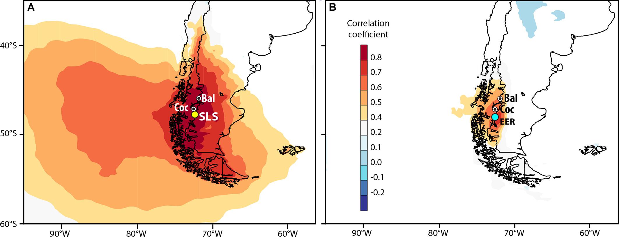
Figure 2. Location of meteorological stations and spatial correlation patterns between monthly anomalies of (A) temperature in San Lorenzo Sur (San Lorenzo Sur), (B) precipitation in Estancia Entre Ríos (EER), and the corresponding anomalies in ERA5.
No precipitation records are available around Monte San Lorenzo. The closest series is from Estancia Entre Ríos (EER- 48.255° S, 72.219° W, 480 m a.s.l.), located approximately 55 km to the south (Figure 2B). Unlike the spatial patterns of temperature, the precipitation correlation fields estimated with the ERA5 records are mostly spatially narrower, particularly on mountainous terrain (Figure 2B). However, the relationships are highly significant (r > 0.6) over the Andes from 45 to 49° S, including in this more spatially limited range the same meteorological stations used for the construction of the regional temperature record. Consequently, the regional precipitation record was based on Balmaceda (1954–2019) and Cochrane (1974–2019). Since the precipitation in Cochrane (total annual 710 mm) is substantially higher than in Balmaceda (total annual 541 mm), the monthly series were normalized and averaged to obtain the regional precipitation departures.
We compared mass balances variations of Río Oro, Río Lácteo, and San Lorenzo Sur glaciers with the seasonal and annual variations of regional temperature and precipitation. To determine the relationships between mass loss and regional climate variations, we averaged the meteorological records for each of the periods in which glacier mass balances were established and conducted comparative analyses with climate data individually for each glacier.
The investigated glaciers retreated and shrunk significantly between 1958 and 2018 (Figures 3, 4 and Table 2). Río Oro, Río Lácteo, and San Lorenzo Sur lost 22 ± 1, 27 ± 1, and 22 ± 1% of their original 1958 area, respectively. This led to an overall glacier area loss rate of 0.46 ± 0.02% a–1 among the three glaciers. In general, the area losses and retreat rates were relatively low before 1981. Whereas Río Oro shrunk at a maximum rate of 0.08 km2 a–1 during the 1981–2000 period, San Lorenzo Sur (0.13 km2 a–1) and Río Lácteo (0.11 km2 a–1) glaciers reached their maximum area loss rate between 2000 and 2012. During this later period, Río Oro and Río Lácteo had the greatest frontal retreat rates (37 and 78 m a–1, respectively). In absolute terms, San Lorenzo Sur had the greatest recession between 1958 and 2018, with total recoil of ∼2762 ± 88 m.
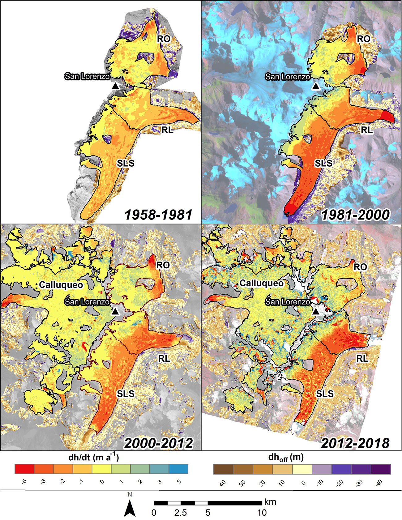
Figure 3. Time-interval glacier annual elevation changes for Rio Oro, Río Lácteo, and San Lorenzo Sur (1958–2018) and the entire San Lorenzo massif (2000–2018). Also shown are elevation changes on stable terrain.
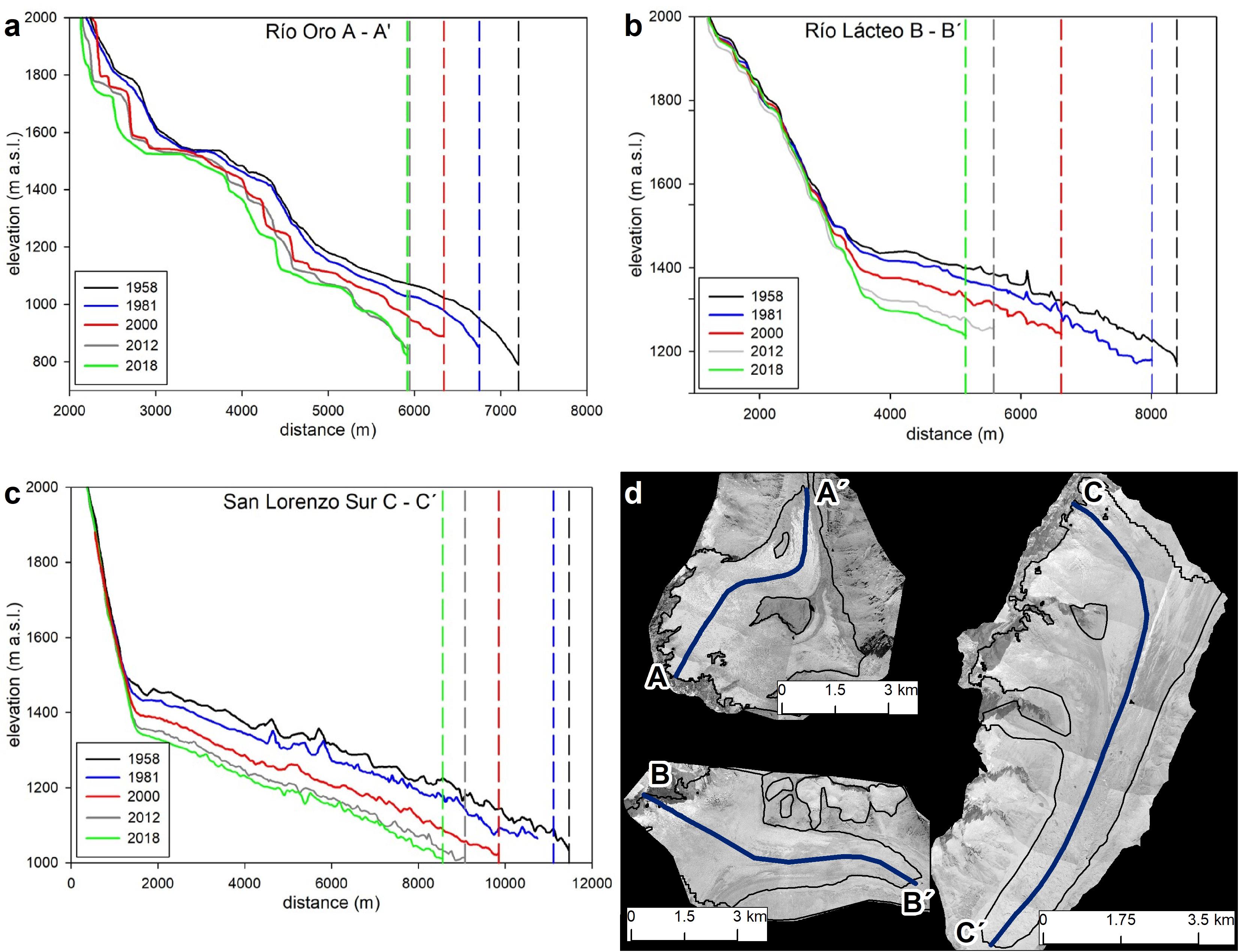
Figure 4. Glacier elevation changes below 2000 m a.s.l. along longitudinal profiles (d) of Río Oro (a), Río Lácteo (b) and San Lorenzo Sur (c). The dashed lines represent glacier frontal positions and in the case of Río Lácteo and San Lorenzo Sur, depict the expansion of proglacial lakes.
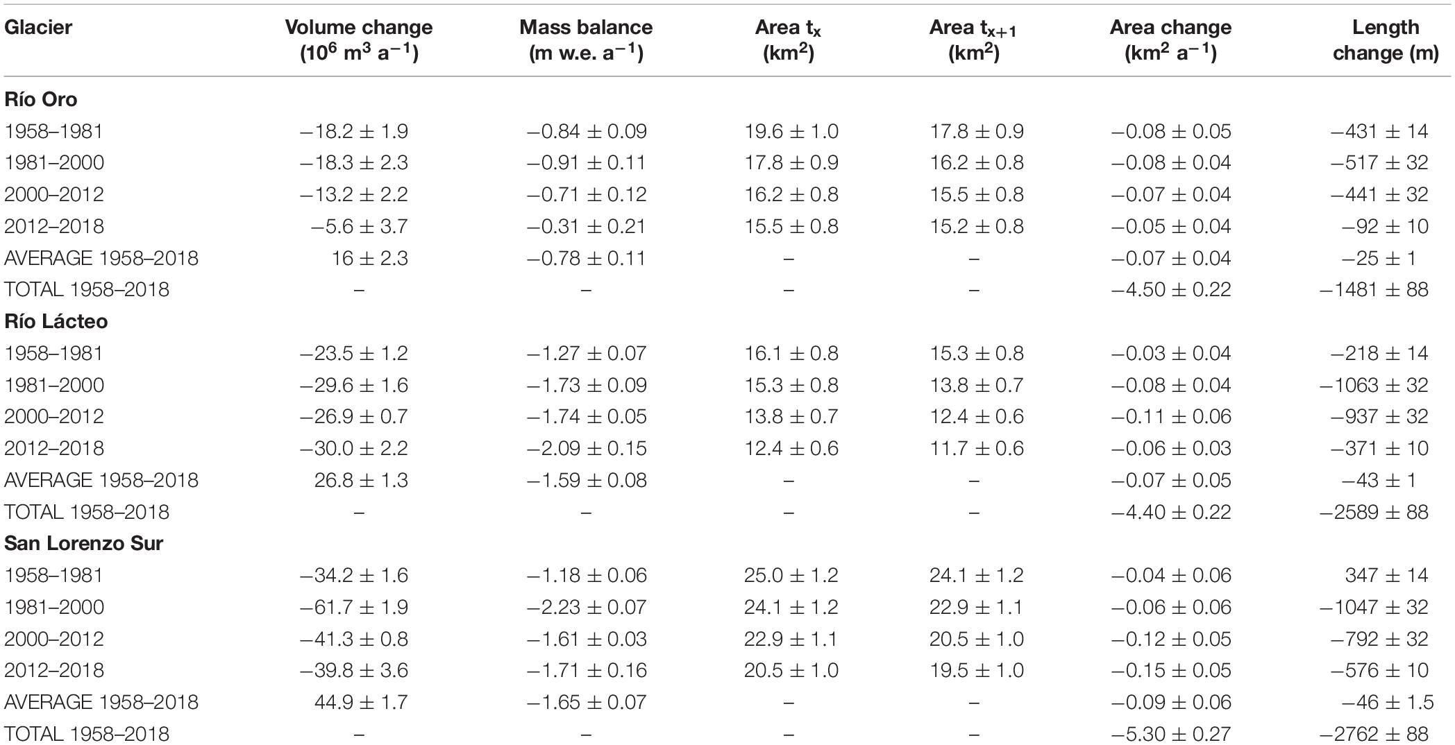
Table 2. Summary of derived glacier change parameters for given time intervals.
As a whole, the Monte San Lorenzo glaciers lost ∼3% area from 2000 to 2012 and further ∼4% area between 2012 and 2018. This is equivalent to a total of 9.54 and 0.53 km2 (about 0.4%) per year since the beginning of the 20th century. Beyond Río Oro, Río Lácteo and San Lorenzo Sur, Calluqueo was the glacier that shrunk the most (−1.16 km2) in absolute and Ventisquero del Comedor (−26%) in relative terms.
Our results show that all three glaciers have significantly thinned and lost mass between 1958 and 2018 (Figures 3–5 and Table 2). Glacier downwasting has led to negative cumulative mass balances of −47.0 ± 6.9 m w.e. [−0.78 ± 0.11 m w.e. a–1] (Río Oro), −95.5 ± 4.8 m w.e. [−1.59 ± 0.08 m w.e. a–1] (Río Lácteo) and −99.1 ± 4.0 m w.e. [−1.65 ± 0.07 m w.e. a–1] (San Lorenzo Sur), whereas the total volume loss was around 5257.5 ± 321.5 × 10⁶ m3 a–1 overall (among the three glaciers) over the 1958–2018 period. Despite the variation in the glacier mass balance during the different time intervals to a certain degree, we found no positive mass balance conditions on any glacier at any investigated time span.
The altitudinal distribution of elevation changes (Figure 5) shows that in general thinning decreases with elevation. Steeper gradients (and more negative absolute values) for all three valley glaciers are observed from the year 1981 onwards compared with the 1958–1981 period, which had a gentler gradient (Figure 5A). This resulted in the least negative overall mass budget (−1.09 ± 0.07 106 m3 a–1) for the initial survey period. For all periods, thinning occurred also at high elevations, indicating that equilibrium line altitudes (ELAs) were rising and accumulation areas were shrinking.
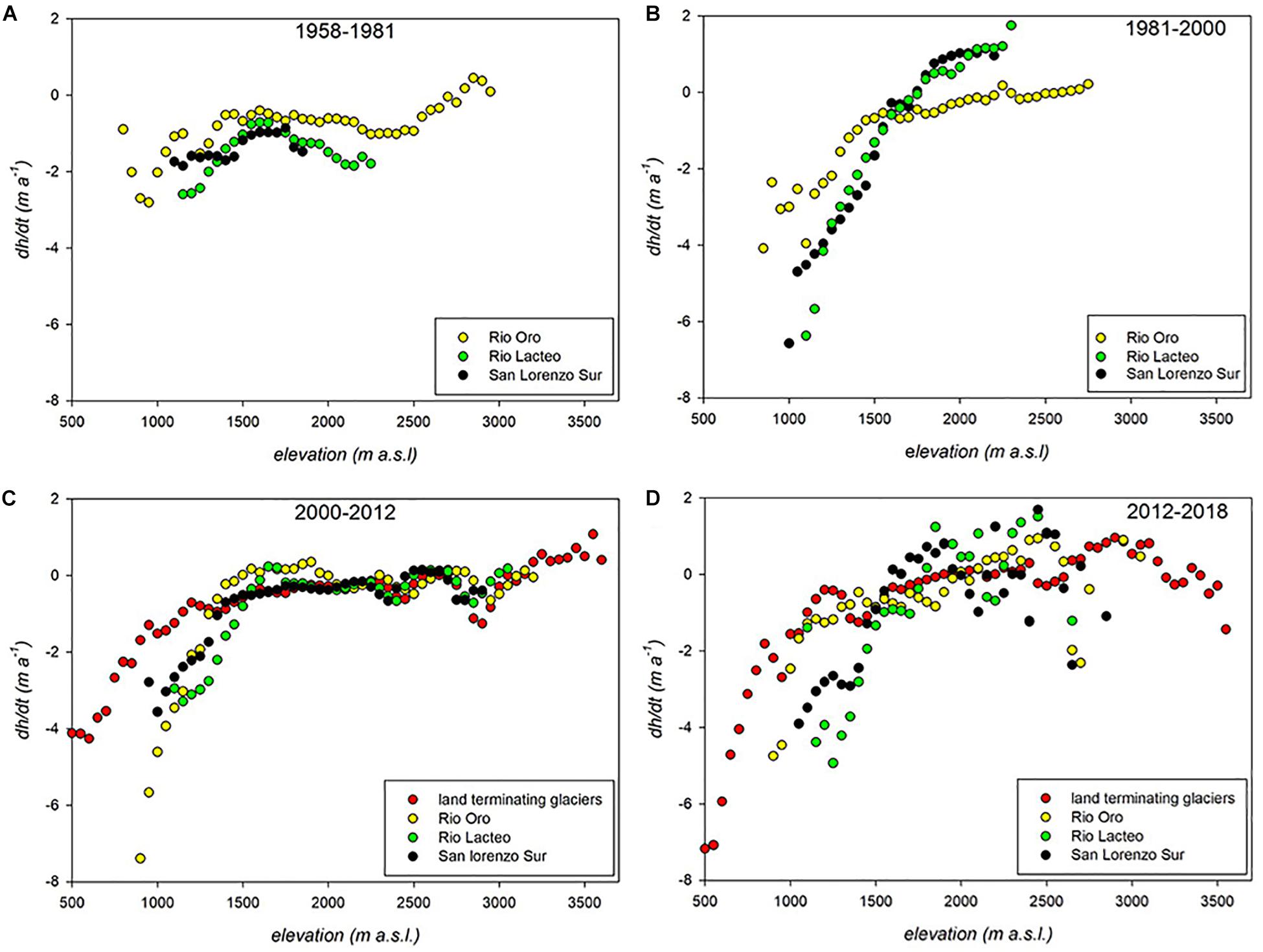
Figure 5. Scatter plot showing glacier elevation change rates as a function of elevation for individual time periods (A–D).
Within the 60-year study period, mass balance conditions were at their most negative during the 1981–2000 time interval (Table 2), with the total ice volume loss reaching a maximum of 109.7 ± 5.8 × 10⁶ m3 a–1. The mass losses for both Río Oro (−0.91 ± 0.11 m w.e. a–1) and San Lorenzo Sur (−2.23 ± 0.07 m w.e. a–1, i.e., the greatest mass loss for a given glacier) peaked during this period. Subsequently, mass loss rates at Río Oro and San Lorenzo Sur have somewhat diminished, resulting in an overall decreased annual volume loss rate of −81.3 ± 3.7 × 10⁶ m3 a–1 (2000–2012) and −75.4 ± 9.5 × 10⁶ m3 a–1 (2012–2018), which is similar to the volume loss rate before 1981 (−75.9 ± 4.8 × 10⁶ m3 a–1).
In comparison with the 2000–2012 time interval, the most recent (2012–2018) mass balance assessment has shown dissimilar mass budget amongst the three valley glaciers: San Lorenzo Sur has maintained analogous conditions, Río Lácteo experienced the greatest mass losses for the whole study period (−2.09 ± 0.15 m w.e. a–1), whilst Río Oro has thinned and lost mass at progressively diminishing rates to an absolute minimum of −0.31 ± 0.21 m w.e. a–1 (2012–2018) (Table 2).
We compared the 2012–2018 mass budget of 15 further glaciers (all land-terminating) in the greater San Lorenzo massif mass budgets against those of the 2000–2012 period. Four glaciers maintained similar values of mass balance, five glaciers had more negative mass balances, while six of them showed more positive values (Table 3). Overall, the mass budget has shifted to a less negative mass balance from −0.31 ± 0.18 to −0.13 ± 0.21 m w.e. a–1.
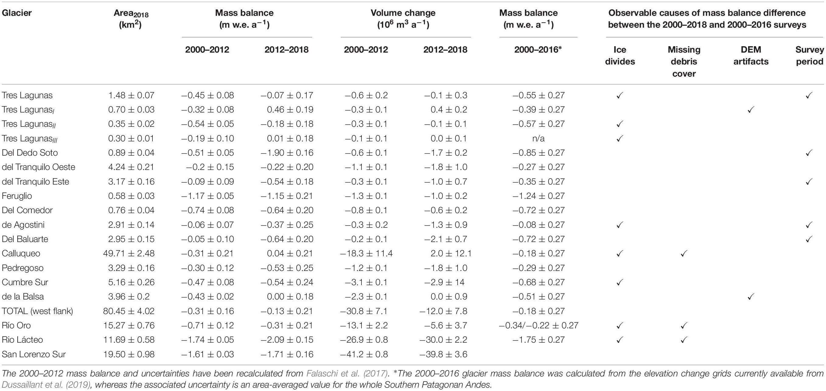
Table 3. Mass budget comparison of 15 land-terminating glaciers in the western side of the main ridge and the three valley glaciers in the east flank of Monte San Lorenzo.
At low elevations (∼1500 m), these 15 mountain glaciers were thinning and losing mass at generally smaller rates when compared to the three main valley glaciers (Figures 5B,C) for a given elevation band, as the lack of calving activity in those smaller, land terminating glaciers results in a minor ice wastage.
Comparison of the monthly deviations of the regional temperature record with those of San Lorenzo Sur shows a strong relation (r = 0.75, p < 0.01) over the 145-month common period (Figure 6A). A highly significant relationship (r = 0.64, p < 0.01) was also found between the monthly variations in the regional precipitation and EER records for the 204-month common period (Figure 6B). This suggests that the regional temperature (1963–2019) and precipitation (1954–2019) records are representative of the climatic variations in Cerro San Lorenzo, and therefore suitable for comparison with the mass balances in the surrounding glaciers.
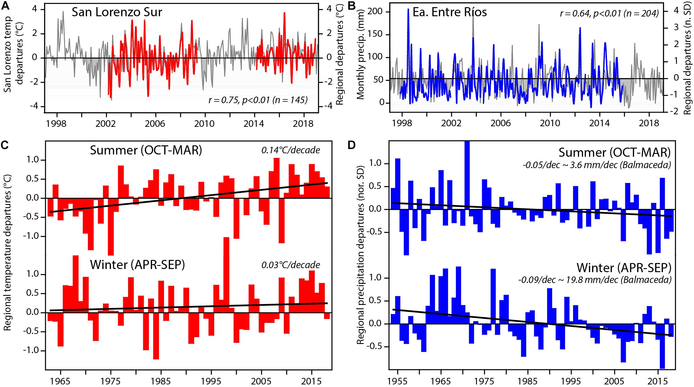
Figure 6. Monthly temperature (A) and precipitation (B) deviations for San Lorenzo Sur (red) and EER (blue) compared to the regional records based on Balmaceda and Cochrane meterorological stations. (C,D) Shows the seasonal (austral summer and winter) monthly temperature (1963–2018) and precipitation (1954–2018) regional departures, respectively. See main text for details.
Temporal variations in regional temperature and precipitation were analyzed seasonally for summer (October–March), winter (April–September), and yearly (April–March). Summer temperatures have increased by 0.8°C from the early 1960s to the present, at a rate of 0.14°C/decade (Figure 6C). In contrast, temperature increases during winter have been more moderate at a rate of 0.03°C/decade (Figure 6C). The summer temperature record shows a marked change from negative to positive deviations in the years 1976–1977 associated with the phase change in the Pacific Decadal Oscillation (see Villalba et al., 2003; Garreaud, 2018). In contrast to summer temperatures, the most important changes in precipitation have been recorded in winter precipitation (Figure 6D). Based on Balmaceda’s seasonal precipitation, reduction rates are 3.6 mm and 19.8 mm/decade for summer and winter, respectively (Figure 6D), representing an annual reduction of around 25 mm/decade approximately from 1954 to the present.
We observed a close relationship between the averaged Río Lácteo and San Lorenzo Sur mass balance and summer temperatures over the 1958–2018 period. The average mass loss per period was used since we noticed a similar mass balance for the Río Lácteo and San Lorenzo Sur glaciers (Table 2), whereas for Río Oro glacier we did not observe a clear relationship between the temporal mass balance evolution and the regional climatic variability.
The period with the least negative mass balance (1958–1981), showing a mean mass loss of −1.23 m w.e. a–1 (−1.27 and −1.18 m w.e. a–1 for Río Lácteo and San Lorenzo Sur), corresponds to negative summer temperature deviations of −0.30°C, relative to the 1963–2019 mean. In contrast, the most negative mass budget of −1.9 m w.e. a–1 (−2.09 and −1.71 m w.e. a–1 for Río Lácteo and San Lorenzo Sur) found for the 2012–2018 interval, was concurrent with a mean summer temperature departure period of + 0.48°C (Figure 7A). It is also worth noting that the reduction in the Río Lácteo-San Lorenzo Sur mass loss rate from −1.98 m w.e. a–1 to −1.68 m w.e. a–1 in 2000 was accompanied by a reduction in summer temperature anomalies between the 1981–2000 and 2000–2012 periods, from 0.16 to 0.09°C, respectively (Figure 7A).
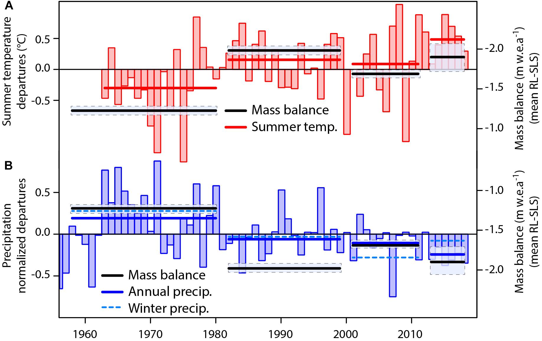
Figure 7. Time-interval variations in glacier mass balance and (A) summer (October–March) temperature and (B) annual/winter precipitation. In the upper (A) panel, the mass balance values on the right axis have been reversed for a better interpretation. Mass balance error bars are shown in the semitransparent boxes.
Similarly, the loss of mass of the Río Lácteo and San Lorenzo Sur glaciers coincided with a decrease in regional rainfall from at least the mid-1950s, when the precipitation record in Balmaceda started (Figure 7B). Total annual rainfalls in the Balmaceda meteorological station were 636, 547, 530, and 455 mm for the 1958–1980, 1981–1999, 2000–2011, and 2012–2018 intervals, respectively. The reduction of total annual precipitation in Balmaceda has been gradual and did not have a recovery period, totalizing a reduction of more than 180 mm between 1958–1980 and 2012–2018.
The overall decrease in winter precipitation (except for the 2012–2018 period) is only consistent with the 1981–2000 shift in mass budget toward more negative conditions (Figure 7B) from −1.23 m w.e. a–1 (1958–1981) to −1.98 m w.e. a–1 (1981−2000).
Correlation analyses between mass balance and climate variables (Table 4) show quite high r values, though they are statistically not significant owed to the small number of observations (just 4 mass balance observation intervals). Summer temperatures (October–March) and annual precipitation show the greatest r values (r = −0.865 and p = 0.135; r = 0.79 and p = 0.20, respectively.
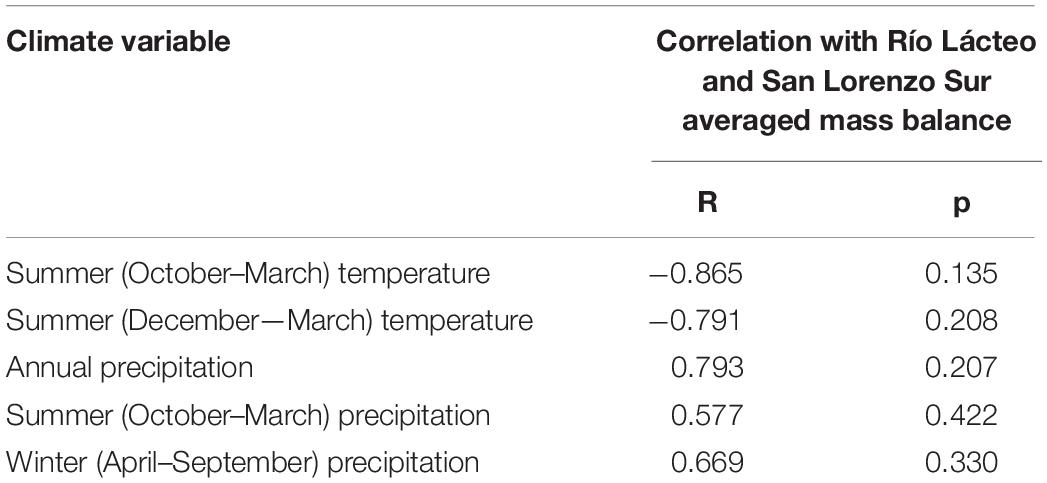
Table 4. Climate and mass balance correlation analyses.
We have seen that the area and mass losses of glaciers in the Monte San Lorenzo area from 1958 to 2018 are consistent with diminishing precipitations and increasing temperatures in the region (Masiokas et al., 2015). This trend of glacier wastage is in line with glacier changes in Southern Patagonia in general (e.g., Mernild et al., 2015; Dussaillant et al., 2018; Braun et al., 2019). The comparison of our mass budget assessment with that of Dussaillant et al. (2019) for the 2000–2016 period (Table 3) shows a relatively good correspondence. At the individual glacier scale, however, some differences arise as a result of (1) different survey time interval (2) local artifacts and data gaps in accumulation regions in the ASTER DEMs (see Dussaillant et al., 2018) or in our own DEMs and particularly (3) the rawness of the Randolph Glacier Inventory outlines used in Dussaillant et al. (2019), which often miss debris covered ice parts and have limitations on the definition of glacier divides, leading to rather different glacier limits. Whilst artifacts and varying ice divides may lead to either positive or negative biases in mass balance (e.g., Tres Lagunas, Cumbre Sur), omitting debris cover ice leads to less negative mass budgets, as debris concentrates in the lowermost parts of glaciers where thinning is usually at the highest. The mass balance of some glaciers (e.g., del dedo Soto, del Tranquilo Este) seems to have changed quite significantly from 2000–2012 to 2012–2018. Consequently, our geodetic mass balance assessment with intermediate points in time (2000-2012-2018) should in principle shed more light on shorter-term variations in comparison with the continuous (2000–2016) survey.
The described pattern of highly negative mass balance conditions at Río Lácteo and San Lorenzo Sur and milder rates at Río Oro and overall of the other 15 mountain glaciers described in Sections “Rio Oro, Río Lácteo, and San Lorenzo Sur 1958–2018 Mass Balance” and “2012–2018 Mass Balance in the Greater San Lorenzo Massif” is consistent throughout the full 1958–2018 period. We interpret these results in view of the different glaciological characteristics such as glacier morphometry, debris cover, ice-calving fronts and supra- and proglacial lakes in particular.
In a regional scale assessment, Falaschi et al. (2017) found significant correlation between mass balance and glacier size (negative) and orientation (positive), implying that on average, the largest, N-NE facing glaciers have the highest thinning rates. Also, we noted a negative correlation between mass balance and slope and no apparent relation between mass balance and median elevation (see also Le Bris and Paul, 2015). These relations emerge from the fact that the larger glaciers in the area (Río Lácteo and San Lorenzo Sur among them) are typically valley glaciers with flatter termini compared with the smaller and steeper mountain glaciers (the mean slope of the San Lorenzo Sur [∼7°] and Río Lácteo [∼8°] tongues, considerably lower than the Río Oro snout [∼18°]) and flow down into the valley floors, where air temperatures are higher and melt rates increase. On the other hand, and in the Southern Hemisphere, N-NE facing slopes receive the most solar radiation, whereas S-SE orientated slopes receive the least and are in the lee side of the prevailing Westerlies.
The aforementioned variable glacier geometry, that in turn affects glacier climatic response, may be further modified by the presence of debris cover and proglacial lakes. Debris cover can lead to more stable glacier tongues (e.g., Scherler et al., 2011; Basnett et al., 2013 and references therein). Whilst the debris cover of Río Lácteo and San Lorenzo Sur were extensive from early on (Figures 8f,k), the lowermost portion of the Río Oro tongue has progressively been covered over time (Figures 8a–e), resulting in decreasing thinning rates. The sheltering effect can be nevertheless removed if glacier tongues are associated with lake expansion (Basnett et al., 2013; King et al., 2019). Under such circumstances, enhanced downwasting of glacier tongues can be promoted by (a) glacier calving on proglacial lakes leading to glacier disintegration (b) supraglacial lakes and thermokarst ponds, as they represent low-albedo spots and (c) gentle slopes resulting in low flow rates at the glacier terminus causing glacier stagnation (Lüthje et al., 2006; Quincey et al., 2007; Bolch et al., 2008). San Lorenzo Sur and Río Lácteo calve indeed into steadily expanding proglacial lakes, and pro-and supraglacial lakes are common on their surface (see Figure 8), whereas neither Río Oro nor the 15 mountain glaciers have proglacial lakes adjoining glacier terminus (Figure 1).
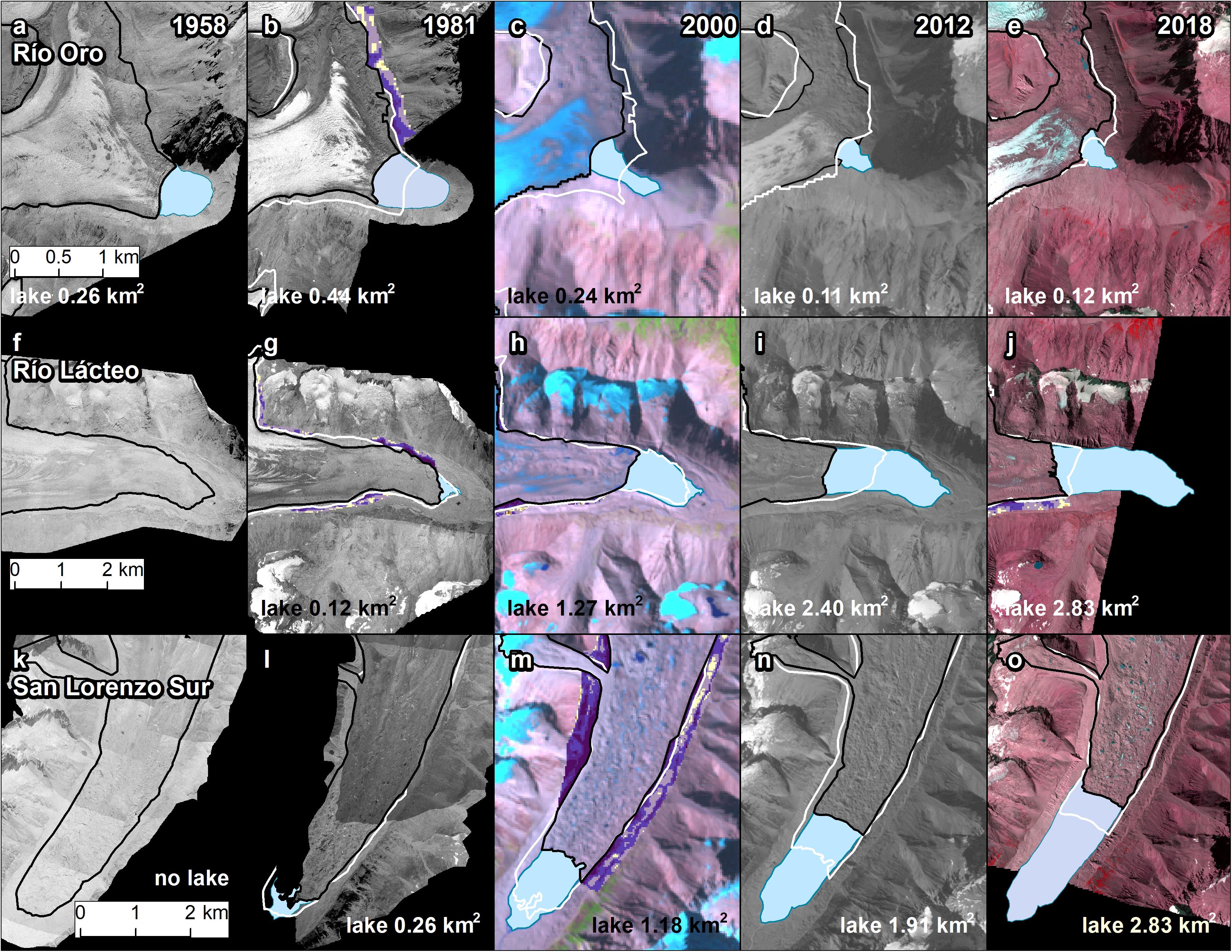
Figure 8. Glacier outline and proglacial lake changes in the Río Oro (a–e), Río Lácteo (f–j), and San Lorenzo Sur (k–o) glaciers. Black lines represent glacier outlines from the actual survey year on each panel and white lines correspond to the previous survey year. The bluish areas adjacent to glacier outlines show the degradation of lateral moraines in response to glacier downwasting (the color scheme is the same as in Figure 3).
The difference in mass budget, owed to the presence of freshwater calving fronts at Río Lácteo and San Lorenzo Sur and the land-terminating northern snout of Río Oro, was already noted by Falaschi et al. (2017). Using the same dataset from these authors, we conducted a t-test and found that in the glacierized area east of the NPI and SPI, the 2000–2012 thinning rate of lake terminating glaciers (−0.88 m a–1) was significantly higher (p < 10–8) than that of land terminating glaciers (−0.27 m a–1) at the 95% confidence level. At an even broader scale, also the outlet glaciers of the SPI and NPI have shrank alongside the increase in debris covered-ice and glacial lake area, whereas for the smaller, mostly debris-free glaciers, no relation was found between the proportion of debris-covered ice and annual rates of glacier retreat (Loriaux and Casassa, 2013; Glasser et al., 2016). Moreover, the negative 1981–2000 Río Lácteo and San Lorenzo Sur mass budget might be underestimated to some extent, as proglacial lake depth has not been accounted for due to the lack of bathymetry data (Bolch et al., 2011a).
To sum up, the 2000–2012 and 2012–2018 mass budgets of Río Lácteo and San Lorenzo Sur are much more negative when put into a wider regional context where land-terminating glaciers prevail (Table 2) whereas the mass budget of Río Oro fits well within the variability of the remaining glaciers in the Monte San Lorenzo (Table 3). We thus suggest that, whilst the overall negative mass budget in the Monte San Lorenzo area is congruent with the observed climatic trends of increasing summer temperatures and decreasing precipitation, the enhanced ablation owed to the presence of proglacial lakes is added or superimposed on the climatic signal, leading to much more negative mass balance values for Río Lácteo and San Lorenzo Sur. Research results in the Himalaya, where glacier-lake interactions are common, concluding that lake-terminating glaciers thin and retreat at a higher rate compared to neighboring land-terminating glaciers (Basnett et al., 2013; Thakuri et al., 2016; King et al., 2018, 2019).
We put forward that the variation in mass balance along the study period is linked to the timing of initiation and expansion of proglacial lakes (Figure 8). In general terms, it can be argued that higher expansion rates are consistent with more negative mass balances, whilst for low rates of expansion, the mass balance seems to be insensitive (Figure 9). Figure 9 also confirms that the San Lorenzo Sur and Río Lácteo mass balance is considerably more negative compared to other glaciers in the area and expansion of their respective proglacial lakes occurs at a much higher rate. A closer look at the San Lorenzo Sur and Río Lácteo lake area values in Figure 8 reveals nonetheless that the relation between thinning rates and lake expansion rates is not straightforward. Before 1981, formation of proglacial lakes was merely incipient (Figures 8b,g,l) and calving presumably limited, hence minor thinning rates were observed. The greatest thinning rates for San Lorenzo Sur occurred between 1981 and 2000, and comparatively minor rates persisted, though the proglacial lake expanded at increasing rates in the subsequent years (0.06–0.15 km a−1, see Figures 8n,o and Table 5). On the other hand, the negative mass budget of Río Lácteo peaked only in the most recent years, and yet the lake expansion rate has remained fairly constant (0.06–0.09 km a–1) since 1981. Such contrasting patterns of glacier thinning and lake area increase were also found in the Himalayas (Basnett et al., 2013; Thakuri et al., 2016). In some instances, however, lake growth can be limited due to steep glacier or headwall topography (Zhang et al., 2019). In the case of Río Lácteo and San Lorenzo Sur, proglacial lakes are mostly developing at the expense of relatively flat glacier tongues, and thus are free to expand further and may eventually coalesce in future years. The onset of calving, following proglacial lake formation, accelerating glacier retreat and thinning is not new for Patagonia, as it had been already acknowledged in the large calving glaciers in the Patagonian Icefields by Warren and Aniya (1999). Moreso, proglacial lakes in Southern Patagonia, have been expanding at increasingly higher rates since the 1980s (Wilson et al., 2018).
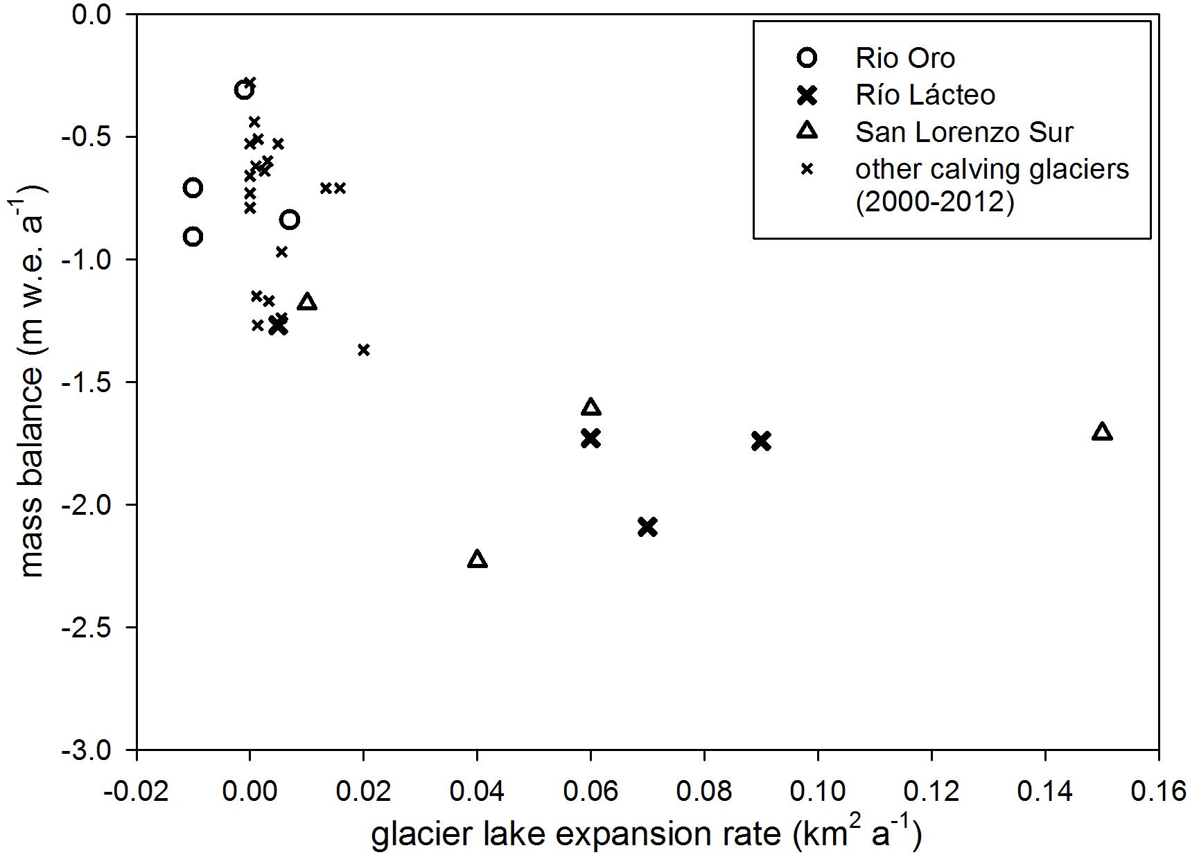
Figure 9. Scatter plot showing the relation between glacier mass balance and proglacial lake expansion rates.
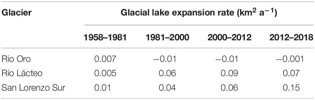
Table 5. Time-interval proglacial lake growth rates.
A proglacial lake has also developed at the southeastern tip of Río Oro glacier but contrary to the proglacial lakes at Río Lácteo (Figures 10a–c) and San Lorenzo Sur, shrunk in area over time although this proglacial lake is deeply confined by terminal moraines and no observable surface drainage system is evident (Figures 8a–d). We hypothesize that water from this small lake has found its way out to the northern terminus of Río Oro glacier via subglacial conduits, following the northward regional slope. The emptying of the lake has been apparently gradual (Table 5), and not sudden as in an ice-dammed lake outburst flood (Glazirin, 2010; Grinsted et al., 2017). This way, the proglacial lake has not expanded further and thinning rates have not increased. In addition to the increasingly larger area covered by debris, we suggest that after an initial period of relatively high thinning and mass loss at lower elevations (Figures 10d,e), Río Oro glacier is rapidly adjusting to present-day climate conditions and thinning rates are largely independent from glacier-lake interactions.
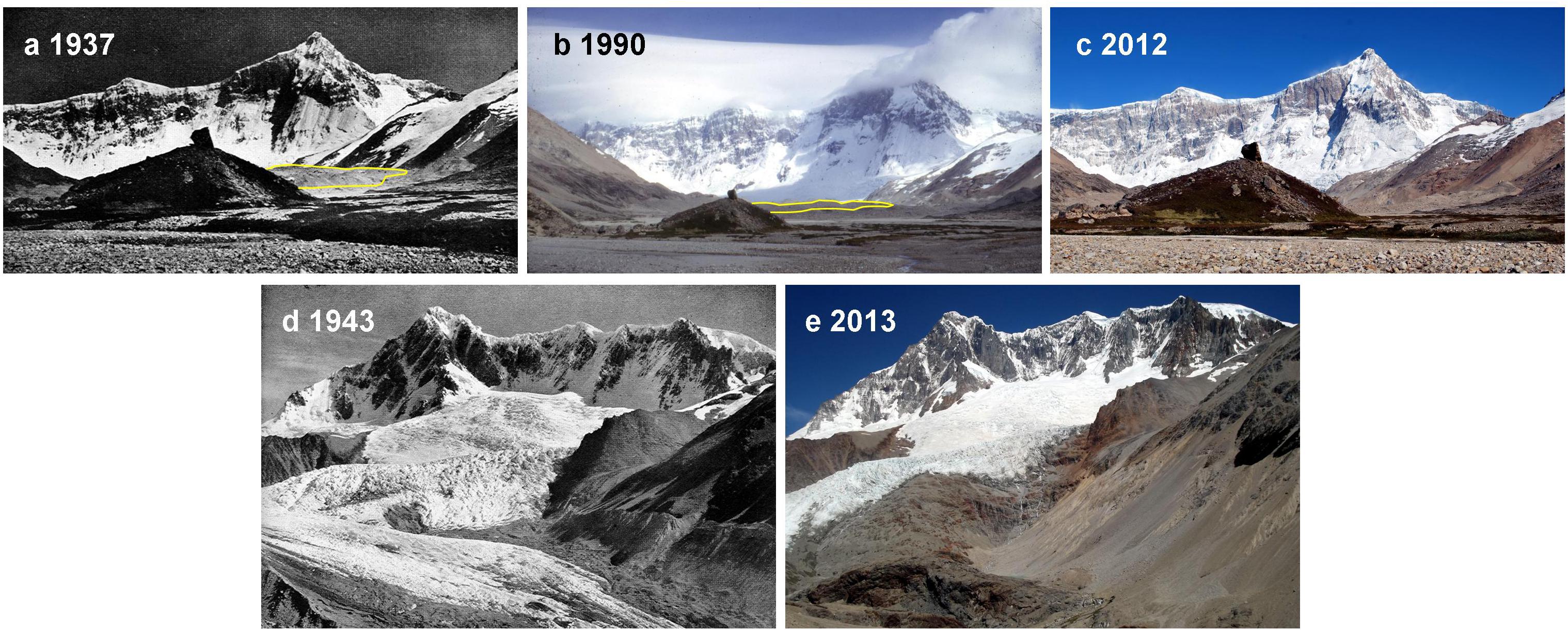
Figure 10. Paired photographs of the Río Lácteo (a–c, in yellow line) and Río Oro (d,e) glaciers. The 1937 and 1943 shots are taken from De Agostini (1945) and the 1990 photo is courtesy of John Mercer.
On a side note, the evolution of these proglacial lakes and glacier area and volume changes must be closely monitored, and the morphometry of its surrounding moraines and valleys evaluated, as potentially dangerous events such as moraine breaching and glacial lake outburst floods (GLOF) need to be identified (Bolch et al., 2011b; Aggarwal et al., 2017; Iribarren Anacona et al., 2015; Wilson et al., 2018; Allen et al., 2019). Slope failure and moraine instability may be induced by stress release in recently deglaciated areas (Cossart et al., 2008) and in effect, certain periods have been characterized by moraine debuttressing at the valley glaciers of Monte San Lorenzo (Figure 8, various panels and Figures 10d,e). Some minor infrastructure of the Perito Moreno National Park (trekkers trails and huts) lie on the outwash plain and fluvial terraces within very few kilometers of the proglacial lake of Río Lácteo (Laguna Témpanos). The area may be hence subjected to the sudden release of a flash flood in case that a large volume of morainic material shall abruptly enter the lake. As a matter of fact, known GLOFs have occurred recently in rapidly deglaciating, not too distant areas (Harrison et al., 2006; Dussaillant et al., 2010) and elsewhere in Patagonia (Worni et al., 2012).
One of the major limitations in glaciological research carried out so far in the Patagonian Andes (45–55° S, sensu Lliboutry, 1956) resides in the fact that the existing records normally initiate after the year 2000 and involve the great outlet glaciers that flow down the Patagonian Icefields but not the smaller, alpine-type glaciers at their margins (Falaschi et al., 2017). These large sea- and lake-terminating glaciers have an inherent cyclic behavior (Rivera et al., 2012), including periods of fast retreat coupled with impressive thinning rates (e.g., Dussaillant et al., 2018; Foresta et al., 2018), which far exceed the observed rates for smaller mountain glaciers nearby (Falaschi et al., 2017). Indeed, these authors found an overall mass loss of 0.46 ± 0.37 m w.e. a–1 for the glaciers located east of the NPI and SPI for the 2000–2012 period, including the Monte San Lorenzo area.
A number of researches concerning Patagonian glaciers whose study period is effectively enclosed in our 1958–2018 time span analysis have been nevertheless carried out at the fresh-water calving Chico (SPI) and Benito (NPI) glaciers. Glaciar Chico thinned at 1.7 ± 0.7 m a–1 on average during 1975–2001 (Rivera et al., 2005). In coincidence with our results from Río Lácteo and San Lorenzo Sur glaciers, the thinning rates determined for Benito glacier before the year 2000 (2.9 ± 0.4 m a–1) were higher than for the 2000–2013 period (1.9 ± 0.7 m a–1). Yet, the approximately quadrupled (7.7 ± 3.0 m a–1) thinning rates between 2013 and 2017 from Benito glacier (Ryan et al., 2018) are contrary to the somewhat diminished thinning values observed for 2012–2018 at Monte San Lorenzo. Post-2000 mass loss at Río Lácteo and San Lorenzo Sur is also comparable to the average losses at the Cordillera Darwin (69° S) in Chile −1.5 ± 0.6 m w.e. a–1; Melkonian et al., 2013) but considerably high in the context of small mountain glaciers outside the Patagonian Icefileds (−0.70 ± 0.32 m w.e. a–1 [NPI] and −0.54 ± 0.17 m w.e. a–1 [SPI]; Braun et al., 2019) and glaciers in Southern Patagonia as a whole (−0.86 ± 0.27 m w.e. a–1; Dussaillant et al., 2019). Regardless of the specific thinning rates, the takeaway message of these contributions in relation to the present study lies in that no periods of positive mass balance conditions have been identified between the year 1973 and 2017, in total agreement with our results from the valley glaciers of Monte San Lorenzo. Also, the mass budget of land-terminating, alpine-type glaciers in the Monte San Lorenzo (−0.31 ± 0.18 and −0.13 ± 0.21 m w.e. a–1) for the 2000–2018 period show analogous values to the early 2000s records available for the Monte Tronador in the northern Patagonian Andes (36–45° S) (−0.17 m w.e. a–1, Ruiz et al., 2017).
We have determined glacier elevation changes and derived a geodetic mass balance of three valley glaciers in the San Lorenzo massif in the Patagonian Andes by differencing DEMs from aerial images, SPOT5 and Pleiades satellite images and the SRTM-X band. This six-decade assessment here represents, to our knowledge, the longest mass balance record in the Southern Andes in general and in Patagonia in particular.
For the entire 1958–2018 study period, we found sustained, negative mass balance conditions at the three investigated valley glaciers. This trend is confirmed by the investigation of 15 more glaciers at the San Lorenzo massif during the more recent 2000–2018 period. Thinning and mass loss maxima among the three valley glaciers occurred during the 1981–2000 period (−1.67 ± 0.11 m w.e. a–1), with a peak of −2.23 ± 0.07 m w.e. a–1 at San Lorenzo Sur. The observed climatic patterns of temperature increase and precipitation decrease over the study period are well-related to the negative mass balance conditions of glaciers in the area. Therefore, the Rio Oro, Río Lácteo, and San Lorenzo Sur glaciers can serve as reference glaciers for future glaciological research and glacier modeling. Most probably, however, feedback mechanisms between proglacial lakes, calving processes and the lowering of the glacier surface found at the Río Lácteo and San Lorenzo Sur tongues, give explanation to the relatively high mass loss rates found at these two glaciers when compared to the land-terminating Río Oro, or the other, smaller mountain glaciers in the Monte San Lorenzo. As a consequence, and whilst the mass budget of the Río Lácteo and San Lorenzo Sur glaciers in recent years (2012–2018) has remained strongly negative, the wider (massif-scale) signal shows a much lower thinning signal, which seems to be closely linked to the climate trends and largely independent from calving or dynamic phenomena. The negative mass balance trend of the last few years nevertheless points out to continuing glacier shrinkage in the Monte San Lorenzo area in particular but also at a broader, regional scale elsewhere in the Patagonian Andes.
The datasets generated for this study are available on request to the corresponding author.
DF designed the study and wrote the manuscript. ML, RV, TB, and AR contributed to the study design and manuscript writing. DF, ML, RV, and AL analyzed the data. All authors contributed to the final version of the manuscript.
This research was funded by the Agencia Nacional de Promoción Científica y Técnica (Grants PICT 2007-0379 and PICT 2016-1282). RV was partially supported by the Foundation BNP-Paribas through THEMES project. AR acknowledges FONDECYT 1171832 and CECs.
The authors declare that the research was conducted in the absence of any commercial or financial relationships that could be construed as a potential conflict of interest.
The Pléiades stereo-pair used in this study was provided by the Pléiades Glacier Observatory (PGO) initiative of the French Space Agency (CNES). Pléiades data© CNES 2018, Distribution Airbus D&S. Special thanks go to Dr. Etienne Berthier for kindly facilitating the inclusion of this research under the PGO program and generating the Pleaides orthorectified products used in this study. The authors would also like to thank Sergio Cimbaro (IGN), Martín Matula (AEROMAPA), and Luis Lenzano and Pierre Pitte (IANIGLA) for handling and scanning the photographic negatives, and the Ohio State University at Columbus, United States, for making available the John Mercer personal archive. Finally, the authors thank AH (associate editor) and two reviewers for their support and valuable comments that helped to improve the final manuscript.
Aggarwal, S. C., Rai, P. K., and Thakur, A. E. (2017). Inventory and recently increasing GLOF susceptibility of glacial lakes in Sikkim, Eastern Himalaya. Geomorphology 295, 39–54. doi: 10.1016/j.geomorph.2017.06.014
Allen, S. K., Zhang, G., Wang, W., Yao, T., and Bolch, T. (2019). Potentially dangerous glacial lakes across the Tibetan Plateau revealed using a large-scale automated assessment approach. Sci. Bull. 64, 435–445. doi: 10.1016/j.scib.2019.03.011
Aniya, M. (2013). Holocene glaciations of Hielo Patagónico (Patagonia Icefield), South America: a brief review. Geochem. J. 47, 97–105. doi: 10.2343/geochemj.1.0171
Bakke, J., and Nesje, A. (2011). “Equilibrium-line-altitude”, in Encyclopedia of Snow, Ice and Glaciers, eds V. Singh, V. P. Singh, and U. Haritashya, (Dordrecht: Springer), 268–277.
Basnett, S., Kulkarni, A. V., and Bolch, T. (2013). The influence of debris cover and glacial lakes on the recession of glaciers in Sikkim Himalaya, India. J. Glaciol. 59, 1035–1046. doi: 10.3189/2013JoG12J184
Berthier, E., Arnaud, Y., Kumar, R., Ahmad, S., Wagnon, P., and Chevallier, P. (2007). Remote sensing estimates of glacier mass balances in the Himachal Pradesh (Western Himalaya, India). Remote Sens. Environ. 108, 327–338. doi: 10.1016/j.rse.2006.11.017
Berthier, E., Larsen, C., Durkin, W. J., Willis, M. J., and Pritchard, M. E. (2018). Brief communication: unabated wastage of the Juneau and Stikine Icefields (Southeast Alaska) in the Early 21st Century. Cryosphere 12, 1523–1530. doi: 10.5194/tc-12-1523-2018
Berthier, E., Vincent, C., Magnússon, E., Gunnlaugsson, Á.Þ., Pitte, P., Le Meur, E., et al. (2014). Glacier topography and elevation changes derived from Pléiades sub-meter stereo images. Cryosphere 8, 2275–2291. doi: 10.5194/tc-8-2275-2014
Bertone, M. (1960). Inventario de los glaciares existentes en la vertiente Argentina entre los paralelos 47° 30’ y 51° S. Buenos Aires: Instituto Nacional del Hielo Continental Patagónico.
Bhambri, R., Bolch, T., Chaujar, R. K., and Kulshreshtha, S. C. (2011). Glacier changes in the Garhwal Himalaya, India, from 1968 to 2006 based on remote sensing. J. Glaciol. 57, 543–556. doi: 10.3189/002214311796905604
Bolch, T., Buchroithner, M. F., Peters, J., Baessler, M., and Bajracharya, S. (2008). Identification of glacier motion and potentially dangerous glacial lakes in the Mt. Everest Region/Nepal using spaceborne imagery. Nat. Hazards Earth Syst. Sci. 8, 1329–1340. doi: 10.5194/nhess-8-1329-2008
Bolch, T., Pieczonka, T., and Benn, D. I. (2011a). Multi-Decadal mass loss of glaciers in the everest area (Nepal Himalaya) derived from stereo imagery. Cryosphere 5, 349–358. doi: 10.5194/tc-5-349-2011
Bolch, T., Peters, J., Yegorov, A., Pradhan, B., Buchroithner, M., and Blagoveshchensky, V. (2011b). Identification of potentially dangerous Glacial Lakes in the Northern Tien Shan. Nat. Hazards 59, 1691–1714. doi: 10.1007/s11069-011-9860-2
Bolch, T., Pieczonka, T., Mukherjee, K., and Shea, J. (2017). Brief communication: glaciers in the Hunza Catchment (Karakoram) have been nearly in balance since the 1970s. Cryosphere 11, 531–539. doi: 10.5194/tc-11-531-2017
Braun, M. H., Malz, P., Sommer, C., Farías-Barahona, D., Sauter, T., Casassa, G., et al. (2019). Constraining glacier elevation and mass changes in South America. Nat. Clim. Change 9, 130–136. doi: 10.1038/s41558-018-0375-7
Brun, F., Wagnon, P., Berthier, E., Jomelli, V., Maharjan, S. B., Shrestha, F., et al. (2019). Heterogeneous influence of glacier morphology on the mass balance variability in high mountain Asia. J. Geophys. Res. Earth Surf. 124, 1331–1345. doi: 10.1029/2018JF004838
Buttstädt, M., Möller, M., Iturraspe, R., and Schneider, C. (2009). Mass balance evolution of martial este glacier, Tierra Del Fuego (Argentina) for the period 1960–2099. Adv. Geosci. 22, 117–124. doi: 10.5194/adgeo-22-117-2009
Carturan, L., Filippi, R., Seppi, R., Gabrielli, P., Notarnicola, C., Bertoldi, L., et al. (2013). Area and volume loss of the glaciers in the ortles-cevedale group (Eastern Italian Alps): controls and imbalance of the remaining glaciers. Cryosphere 7, 1339–1359. doi: 10.5194/tc-7-1339-2013
Cogley, J. G. (2009). Geodetic and direct mass-balance measurements: comparison and joint analysis. Ann. Glaciol. 50, 96–100. doi: 10.3189/172756409787769744
Corte, A. E., and Espizúa, L. (1981). Inventario de Glaciares del la Cuenca del río Mendoza. Mendoza: IANIGLA-CONICET.
Cossart, E., Braucher, R., Fort, M., Bourlés, D. L., and Carcaillet, J. (2008). Slope instability in relation to glacial debuttressing in alpine areas (Upper Durance catchment, southeastern France): evidence from field data and 10Be cosmic ray exposure ages. Geomorphology 95, 3–26. doi: 10.1016/j.geomorph.2006.12.022
Cox, L. H., and March, R. S. (2004). Comparison of geodetic and glaciological mass-balance techniques, Gulkana Glacier, Alaska, U.S.A. J. Glaciol. 50, 363–370. doi: 10.3189/172756504781829855
Davies, B. J., and Glasser, N. F. (2012). Accelerating shrinkage of patagonian glaciers from the little ice age (~AD 1870) to 2011. J. Glaciol. 58, 1063–1084. doi: 10.3189/2012JoG12J026
De Agostini, A. M. (1945). Andes Patagónicos: Viajes de exploración a la cordillera patagónica austral. Buenos Aires: Talleres Gráficos de Guillermo Kraft.
Dussaillant, A., Benito, G., Buytaert, W., Carling, P., Meier, C., and Espinoza, F. (2010). Repeated glacial-lake outburst floods in Patagonia: an increasing hazard? Nat. Hazards 54, 469–481. doi: 10.1007/s11069-009-9479-8
Dussaillant, I., Berthier, E., and Brun, F. (2018). Geodetic mass balance of the Northern Patagonian Icefield from 2000 to 2012 using two independent methods. Front. Earth Sci. 6:8. doi: 10.3389/feart.2018.00008
Dussaillant, I., Berthier, E., Brun, F., Masiokas, M., Hugonnet, R., Favier, V., et al. (2019). Two decades of glacier mass loss along the Andes. Nat. Geosci. 12, 802–808. doi: 10.1038/s41561-019-0432-5
Espizúa, L. (1983). “Glacier and moraine inventory on the eastern slopes of Cordón del Plata and Cordón del Portillo, Central Andes, Argentina,” in Tills and Related Deposits, eds E. B. Evenson, J. Rabassa, and Schlüchter, (Avereest: Balkema), 381–395.
Falaschi, D., Bolch, T., Lenzano, M. G., Tadono, T., Lo Vecchio, A., and Lenzano, L. (2018). New evidence of glacier surges in the central andes of Argentina and Chile. Prog. Phys. Geogr. Earth Environ. 42, 792–825. doi: 10.1177/0309133318803014
Falaschi, D., Bolch, T., Rastner, P., Lenzano, M. G., Lenzano, L., Lo Vecchio, A., et al. (2017). Mass changes of Alpine Glaciers at the Eastern Margin of the Northern and Southern Patagonian Icefields between 2000 and 2012. J. Glaciol. 63, 258–272. doi: 10.1017/jog.2016.136
Falaschi, D., Bravo, C., Masiokas, M., Villalba, R., and Rivera, A. (2013). First Glacier inventory and recent changes in glacier area in the monte San Lorenzo Region (47°S), Southern Patagonian Andes, South America. Arct. Antarct. Alp. Res. 45, 19–28. doi: 10.1657/1938-4246-45.1.19
Farías-Barahona, D., Vivero, S., Casassa, G., Schaefer, M., Burger, F., Seehaus, T., et al. (2019). Geodetic mass balances and area changes of Echaurren Norte Glacier (Central Andes, Chile) between 1955 and 2015. Remote Sens. 11:260. doi: 10.3390/rs11030260
Fieber, K. D., Mills, J. P., Miller, P. E., Clarke, L., Ireland, L., and Fox, A. J. (2018). Rigorous 3D change determination in Antarctic Peninsula Glaciers from stereo WorldView-2 and Archival Aerial Imagery. Remote Sens. Environ. 205, 18–31. doi: 10.1016/j.rse.2017.10.042
Fischer, A. (2011). Comparison of direct and geodetic mass balances on a multi-annual time scale. Cryosphere 5, 107–124. doi: 10.5194/tc-5-107-2011
Fischer, M., Huss, M., and Hoelzle, M. (2015). Surface elevation and mass changes of all swiss glaciers 1980–2010. Cryosphere 9, 525–540. doi: 10.5194/tc-9-525-2015
Foresta, L., Gourmelen, N., Weissgerber, F., Nienow, P., Williams, J. J., Shepherd, A., et al. (2018). Heterogeneous and rapid ice loss over the patagonian ice fields revealed by Cryosat-2 Swath Radar altimetry. Remote Sens. Environ. 211, 441–455. doi: 10.1016/j.rse.2018.03.041
Gardelle, J., Berthier, E., Arnaud, Y., and Kääb, A. (2013). Region-Wide Glacier mass balances over the Pamir-Karakoram-Himalaya during 1999-2011. Cryosphere 7, 1263–1286. doi: 10.5194/tc-7-1263-2013
Gardner, A. S., Moholdt, G., Cogley, J. G., Wouters, B., Arendt, A. A., Wahr, J., et al. (2013). A reconciled estimate of glacier contributions to sea level rise: 2003 to 2009. Science 340, 852–857. doi: 10.1126/science.1234532
Garibotti, I. A., and Villalba, R. (2017). Colonization of mid- and late-holocene moraines by lichens and trees in the magellanic sub-antarctic province. Pol. Biol. 40, 1739–1753. doi: 10.1007/s00300-017-2096-1
Garreaud, R., López, P., Minvielle, M., and Rojas, M. (2013). Large scale control on the Patagonia climate. J. Clim. 26, 215–230. doi: 10.1175/JCLI-D-12-001.1
Garreaud, R. D. (2009). The andes climate and weather. Adv. Geosci. 22, 3–11. doi: 10.5194/adgeo-22-3-2009
Garreaud, R. D. (2018). Record-breaking climate anomalies lead to severe drought and environmental disruption in Western Patagonia in 2016. Clim. Res. 74, 217–229. doi: 10.3354/cr01505
Glasser, N. F., Holt, T. O., Evans, Z. D., Davies, B. J., Pelto, M., and Harrison, S. (2016). Recent spatial and temporal variations in debris cover on Patagonian glaciers. Geomorphology 273, 202–216. doi: 10.1016/j.geomorph.2016.07.036
Glasser, N. F., and Jansson, K. N. (2008). The Glacial Map of southern South America. J. Maps 4, 175–196. doi: 10.4113/jom.2008.102
Glazirin, G. (2010). A century of investigations on outbursts of the ice-dammed lake Merzbacher (central Tien Shan). Aust. J. Earth Sci. 103, 171–179.
Grinsted, A., Hvidberg, C. S., Campos, N., and Dahl-Jensen, D. (2017). Periodic outburst floods from an Ice-Dammed Lake in East Greenland. Sci. Rep. 7:9966. doi: 10.1038/s41598-017-07960-9
Hall, D. K., Bayr, K. J., Schöner, W., Bindschadler, R. A., and Chien, J. Y. L. (2003). Consideration of the errors inherent in mapping historical glacier positions in Austria from the ground and space (1893–2001). Remote Sens. Environ. 86, 566–577. doi: 10.1016/S0034-4257(03)00134-2
Harrison, S., Glasser, N., Winchester, V., Haresign, E., Warren, C., and Jansson, K. (2006). A glacial lake outburst flood associated with recent mountain glacier retreat, patagonian andes. Holocene 16, 611–620. doi: 10.1191/0959683606hl957rr
Huss, M. (2013). Density assumptions for converting geodetic glacier volume change to mass change. Cryosphere 7, 877–887. doi: 10.5194/tc-7-877-2013
Iribarren Anacona, P., Mackintosh, A., and Norton, K. P. (2015). Hazardous processes and events from glacier and permafrost areas: lessons from the Chilean and Argentinean Andes. Earth Surf. Process. Landf. 40, 2–21. doi: 10.1002/esp.3524
Kerner, S., Kaufman, I., and Raizman, Y. (2016). “Role of Tie-Points distribution in aerial photography,” in Proccedings of the ISPRS International Archives of the Photogrammetry, Remote Sensing and Spatial Information Sciences XL-3/W4, Lausanne, 41–44. doi: 10.5194/isprsarchives-XL-3-W4-41-2016
King, O., Bhattacharya, A., Bhambri, R., and Bolch, T. (2019). Glacial lakes exacerbate Himalayan glacier mass loss. Sci. Rep. 9:18145. doi: 10.1038/s41598-019-53733-x
King, O., Dehecq, A., Quincey, D., and Carrivick, J. (2018). Contrasting geometric and dynamic evolution of lake and land-terminating Glaciers in the Central Himalaya. Glob. Planet. Change 167, 46–60. doi: 10.1016/j.gloplacha.2018.05.006
Koblet, T., Gärtner-Roer, I., Zemp, M., Jansson, P., Thee, P., Haeberli, W., et al. (2010). Reanalysis of multi-temporal aerial images of storglaciären, Sweden (1959-99) Part 1: determination of length, area, and volume changes. Cryosphere 4, 333–343. doi: 10.5194/tc-4-333-2010
Korona, J., Berthier, E., Bernard, M., Rémy, F., and Thouvenot, E. (2009). SPIRIT. SPOT 5 stereoscopic survey of Polar Ice: reference images and Topographies during the Fourth International Polar Year (2007–2009). ISPRS J. Photogramm. Remote Sens. 64, 204–212. doi: 10.1016/j.isprsjprs.2008.10.005
Le Bris, R., and Paul, F. (2015). Glacier-specific elevation changes in parts of western Alaska. Ann. Glaciol. 56, 184–192. doi: 10.3189/2015AoG70A227
Lenzano, M. G. (2013). Assessment of using ASTER-Derived DTM for glaciological applications in the Central Andes, Mt. Aconcagua, Argentina. Photogramm. Fernerkundung Geoinformation 3, 197–208. doi: 10.1127/1432-8364/2013/0170
Lliboutry, L. (1956). Nieves y glaciares de Chile, fundamentos de glaciología. [Snow and glaciers of Chile, foundations of glaciology]. Santiago de Chile: Universidad de Chile.
Loriaux, T., and Casassa, G. (2013). Evolution of Glacial Lakes from the Northern Patagonia Icefield and Terrestrial Water Storage in a Sea-Level Rise Context. Glob. Planet. Change 102, 33–40. doi: 10.1016/j.gloplacha.2012.12.012
Lüthje, M., Pedersen, L. T., Reeh, N., and Greuell, W. (2006). Modelling the evolution of Supraglacial Lakes on the West Greenland Ice-Sheet Margin. J. Glaciol. 52, 608–618. doi: 10.3189/172756506781828386
Marzeion, B., Jarosch, A. H., and Hofer, M. (2012). Past and future sea-level change from the surface mass balance of glaciers. Cryosphere 6, 1295–1322. doi: 10.5194/tc-6-1295-2012
Masiokas, M. H., Delgado, S., Pitte, P., Berthier, E., Villalba, R., Skvarca, P., et al. (2015). Inventory and recent changes of small glaciers on the Northeast Margin of the Southern Patagonia Icefield, Argentina. J. Glaciol. 61, 511–523. doi: 10.3189/2015JoG14J094
Maurer, J. M., Schaefer, J. M., Rupper, S., and Corley, A. (2019). Acceleration of Ice Loss across the Himalayas over the Past 40 Years. Sci. Adv. 5:eaav7266. doi: 10.1126/sciadv.aav7266
McNabb, R., Nuth, C., Kääb, A., and Girod, L. (2019). Sensitivity of glacier volume change estimation to DEM void interpolation. Cryosphere 13, 895–910. doi: 10.5194/tc-13-895-2019
Melkonian, A. K., Willis, M. J., Pritchard, M. E., Rivera, A., Bown, F., and Bernstein, S. A. (2013). Satellite-derived volume loss rates and glacier speeds for the cordillera darwin icefield, Chile. Cryosphere 7, 823–839. doi: 10.5194/tc-7-823-2013
Mercer, J. H. (1968). Variations of some Patagonian glaciers since the Late-Glacial. Am. J. Sci. 266, 91–109. doi: 10.2475/ajs.266.2.91
Mernild, S. H., Beckerman, A. P., Yde, J. C., Hanna, E., Malmros, J. K., Wilson, R., et al. (2015). Mass loss and imbalance of glaciers along the andes cordillera to the Sub-Antarctic Islands. Glob. Planet. Change 133, 109–119. doi: 10.1016/j.gloplacha.2015.08.009
Mölg, N., and Bolch, T. (2017). Structure-from-Motion using historical aerial images to analyse changes in glacier surface elevation. Remote Sens. 9:1021. doi: 10.3390/rs9101021
Mölg, N., Bolch, T., Walter, A., and Vieli, A. (2019). Unravelling the evolution of zmuttgletscher and its debris cover since the end of the little ice age. Cryosphere 13, 1889–1909. doi: 10.5194/tc-13-1889-2019
Morano-Büchner, C., and Aravena, J. C. (2013). Lichenometric analysis using genus Rhizocarpon, section Rhizocarpon (Lecanorales: Rhizocarpaceae) at Mount San Lorenzo, southern Chile. Rev. Chil. Hist. Nat. 86, 465–473. doi: 10.4067/s0716-078x2013000400008
Nuth, C., and Kääb, A. (2011). Co-Registration and bias corrections of satellite elevation data sets for quantifying glacier thickness change. Cryosphere 5, 271–290. doi: 10.5194/tc-5-271-2011
Paul, F., Barrand, N. E., Baumann, S., Berthier, E., Bolch, T., Casey, K., et al. (2013). On the accuracy of glacier outlines derived from remote-sensing data. Ann. Glaciol. 54, 171–182. doi: 10.3189/2013AoG63A296
Paul, F., Barry, R. G., Cogley, J. G., Frey, H., Haeberli, W., Ohmura, A., et al. (2009). Recommendations for the compilation of glacier inventory data from digital sources. Ann. Glaciol. 50, 119–126. doi: 10.3189/172756410790595778
Paul, F., and Mölg, N. (2014). Hasty retreat of glaciers in northern patagonia from 1985 to 2011. J. Glaciol. 60, 1033–1043. doi: 10.3189/2014JoG14J104
Pieczonka, T., and Bolch, T. (2015). Region-Wide glacier mass budgets and area changes for the central tien shan between ~1975 and 1999 using Hexagon KH-9 imagery. Glob. Planet. Change 128, 1–13. doi: 10.1016/j.gloplacha.2014.11.014
Pieczonka, T., Bolch, T., and Buchroithner, M. (2011). Generation and evaluation of multitemporal digital terrain models of the Mt. Everest area from different optical sensors. ISPRS J. Photogramm. Remote Sens. 66, 927–940. doi: 10.1016/j.isprsjprs.2011.07.003
Popovnin, V., Tatyana, V., Danilova, A., and Petrakov, D. A. (1999). Pioneer mass balance estimate for a patagonian glacier: glaciar De Los Tres, Argentina. Glob. Planet. Change 22, 255–267. doi: 10.1016/S0921-8181(99)00042-9
Quincey, D. J., Richardson, S. D., Luckman, A., Lucas, R. M., Reynolds, J. M., Hambrey, M. J., et al. (2007). Early recognition of glacial lake hazards in the himalaya using remote sensing datasets. Glob. Planet. Change 56, 137–152. doi: 10.1016/j.gloplacha.2006.07.013
Racoviteanu, A. E., Yves, A., Williams, M. W., and Manley, W. F. (2015). Spatial patterns in glacier characteristics and area changes from 1962 to 2006 in the Kanchenjunga–Sikkim area, eastern Himalaya. Cryosphere 9, 505–523. doi: 10.5194/tc-9-505-2015
Ragettli, S., Bolch, T., and Pellicciotti, F. (2016). Heterogeneous glacier thinning patterns over the last 40 years in LangtangHimal, Nepal. Cryosphere 10, 2075–2097. doi: 10.5194/tc-10-2075-2016
Rignot, E., Rivera, A., and Casassa, G. (2003). Contribution of the Patagonia Icefields of South America to Sea Level Rise. Science 302, 434–437. doi: 10.1126/science.1087393
Rivera, A., Benham, T., Casassa, G., Bamber, J., and Dowdeswell, J. A. (2007). Ice Elevation and Areal Changes of Glaciers from the Northern Patagonia Icefield, Chile. Glob. Planet. Change 59, 126–137. doi: 10.1016/j.gloplacha.2006.11.037
Rivera, A., Casassa, G., Bamber, J., and Kääb, A. (2005). Ice-Elevation changes of glaciar chico, southern patagonia, using ASTER DEMs, aerial photographs and GPS data. J. Glaciol. 51, 105–112. doi: 10.3189/172756505781829557
Rivera, A., Corripio, J., Bravo, C., and Cisternas, S. (2012). Glaciar jorge montt (chilean patagonia) dynamics derived from photos obtained by fixed cameras and satellite image feature tracking. Ann. Glaciol. 53, 147–155. doi: 10.3189/2012AoG60A152
Rolstad, C., Haug, T., and Denby, B. (2009). Spatially integrated geodetic glacier mass balance and its uncertainty based on geostatistical analysis: application to the western Svartisen ice cap, Norway. J. Glaciol. 55, 666–680. doi: 10.3189/002214309789470950
Ruiz, L., Berthier, E., Viale, M., Pitte, P., and Masiokas, M. (2017). Recent geodetic mass balance of monte tronador glaciers, North Patagonian Andes. Cryosphere 11, 619–634. doi: 10.5194/tc-11-619-2017
Ryan, J. C., Sessions, M., Wilson, R., Wündrich, O., and Hubbard, A. (2018). Rapid surface lowering of benito glacier, Northern Patagonian Icefield. Front. Earth Sci. 6:47. doi: 10.3389/feart.2018.00047
Sagredo, E. A., and Lowell, T. V. (2012). Climatology of Andean glaciers: a framework to understand glacier response to climate change. Glob. Planet. Change 8, 101–109. doi: 10.1016/j.gloplacha.2012.02.010
Sagredo, E. A., Lowell, T. V., Kelly, M. A., Rupper, S., Aravena, J. C., Ward, D. J., et al. (2017). Equilibrium line altitudes along the Andes during the Last millennium: paleoclimatic implications. Holocene 27, 1019–1033. doi: 10.1177/0959683616678458
Sapiano, J. J., Harrison, W. D., and Echelmeyer, K. A. (1998). Elevation, volume and terminus changes of nine glaciers in North America. J. Glaciol. 44, 119–135. doi: 10.3189/S0022143000002410
Scherler, D., Bookhagen, B., and Strecker, M. R. (2011). Spatially variable response of himalayan glaciers to climate change affected by debris cover. Nat. Geosci. 4, 156–159. doi: 10.1038/ngeo1068
Schmidt, S., and Nüsser, M. (2017). Changes of high altitude glaciers in the Trans-Himalaya of Ladakh over the Past Five Decades (1969–2016). Geosciences 7:27. doi: 10.3390/geosciences7020027
Schwikowski, M., Schläppi, M., Santibañez, P., Rivera, A., and Casassa, G. (2013). Net accumulation rates derived from ice core stable isotope records of Pío XI Glacier, Southern Patagonia Icefield. Cryosphere 7, 1635–1644. doi: 10.5194/tc-7-1635-2013
Shean, D. E., Alexandrov, O., Moratto, Z. M., Smith, B. E., Joughin, I. R., Porter, C., et al. (2016). An automated, open-source pipeline for mass production of digital elevation models (DEMs) from very-high-resolution commercial stereo satellite imagery. ISPRS J. Photogramm. Remote Sens. 116, 101–117. doi: 10.1016/j.isprsjprs.2016.03.012
Strelin, J. A., and Iturraspe, R. (2007). Recent evolution and mass balance of Cordón Martial glaciers. Cordillera Fueguina Oriental. Glob. Planet. Change 59, 17–26. doi: 10.1016/j.gloplacha.2006.11.019
Thakuri, S., Salerno, F., Bolch, T., Guyennon, N., and Tartari, G. (2016). Factors controlling the accelerated expansion of Imja Lake, Mount Everest region, Nepal. Ann. Glaciol. 57, 245–257. doi: 10.3189/2016AoG71A063
Vargo, L., Amderson, B., Horgan, H., Mackintosh, A., Lorrey, A., and Thornton, M. (2017). Using structure from motion photogrammetry to measure past glacier changes from historic aerial photographs. J. Glaciol. 63, 1105–1118. doi: 10.1017/jog.2017.79
Villalba, R., Lara, A., Boninsegna, J. A., Masiokas, M., Delgado, S., Aravena, J. C., et al. (2003). Large-scale temperature changes across the southern Andes: 20th-century variations in the context of the past 400 years. Clim. Change 59, 177–232. doi: 10.1007/978-94-015-1252-7_10
Warren, C., and Aniya, M. (1999). The calving glaciers of southern South America. Glob. Planet. Change 22, 59–77. doi: 10.1016/S0921-8181(99)00026-0
Wenzens, G. (2002). The influence of tectonically derived relief and climate on the extent of the last glaciation east of the Patagonian ice fields (Argentina, Chile). Tectonophysics 345, 329–344. doi: 10.1016/S0040-1951(01)00219-0
WGMS (2017). “Global glacier change bulletin no. 2 (2014-2015),” in ICSU(WDS)/IUGG(IACS)/UNEP/UNESCO/WMO, eds M. Zemp, S. U. Nussbaumer, I. Gärtner-Roer, J. Huber, H. Machguth, F. Paul, et al. (Zürich: World Glacier Monitoring Service). doi: 10.5904/wgms-fog-2017-06
Willis, M. J., Melkonian, A. K., Pritchard, M. E., and Rivera, A. (2012). Ice loss from the Southern Patagonian Ice Field, South America, between 2000 and 2012. Geophys. Res. Lett. 39:L17501. doi: 10.1029/2012GL053136
Wilson, R., Glasser, N. F., Reynolds, J. M., Harrison, S., Iribarren Anacona, P., Schaefer, M., et al. (2018). Glacial lakes of the Central and Patagonian Andes. Glob. Planet. Change 162, 275–291. doi: 10.1016/j.gloplacha.2018.01.004
Wolff, I. W., Glasser, N., and Hubbard, A. (2013). The reconstruction and climatic implication of an independent palaeo ice cap within the Andean rain shadow east of the former Patagonian ice sheet, Santa Cruz Province, Argentina. Geomorphology 185, 1–15. doi: 10.1016/j.geomorph.2012.10.018
Worni, R., Stoffel, M., Huggel, C., Volz, C., Casteller, A., and Luckman, B. (2012). Analysis and dynamic modeling of a moraine failure and glacier lake outburst flood at Ventisquero Negro, Patagonian Andes (Argentina). J. Hydrol. 444–445, 134–145. doi: 10.1016/j.jhydrol.2012.04.013
Zemp, M., Huss, M., Thibert, E., Eckert, N., McNabb, R., Huber, J., et al. (2019). Global glacier mass changes and their contributions to sea-level rise from 1961 to 2016. Nature 568, 382–386. doi: 10.1038/s41586-019-1071-0
Keywords: geodetic mass balance, glacier retreat, glacial lake, Monte San Lorenzo, Patagonian Andes
Citation: Falaschi D, Lenzano MG, Villalba R, Bolch T, Rivera A and Lo Vecchio A (2019) Six Decades (1958–2018) of Geodetic Glacier Mass Balance in Monte San Lorenzo, Patagonian Andes. Front. Earth Sci. 7:326. doi: 10.3389/feart.2019.00326
Received: 01 August 2019; Accepted: 27 November 2019;
Published: 11 December 2019.
Edited by:
Alun Hubbard, Arctic University of Norway, NorwayReviewed by:
David Loibl, Humboldt University of Berlin, GermanyCopyright © 2019 Falaschi, Lenzano, Villalba, Bolch, Rivera and Lo Vecchio. This is an open-access article distributed under the terms of the Creative Commons Attribution License (CC BY). The use, distribution or reproduction in other forums is permitted, provided the original author(s) and the copyright owner(s) are credited and that the original publication in this journal is cited, in accordance with accepted academic practice. No use, distribution or reproduction is permitted which does not comply with these terms.
*Correspondence: Daniel Falaschi, ZGZhbGFzY2hpQG1lbmRvemEtY29uaWNldC5nb3YuYXI=
Disclaimer: All claims expressed in this article are solely those of the authors and do not necessarily represent those of their affiliated organizations, or those of the publisher, the editors and the reviewers. Any product that may be evaluated in this article or claim that may be made by its manufacturer is not guaranteed or endorsed by the publisher.
Research integrity at Frontiers
Learn more about the work of our research integrity team to safeguard the quality of each article we publish.