 Janet Cristine Richardson
 David Mark Hodgson
 Paul Kay2
 Benjamin J. Aston
- 1Stratigraphy Group, School of Earth and Environment, University of Leeds, Leeds, United Kingdom
- 2School of Geography, University of Leeds, Leeds, United Kingdom
- 3Yorkshire Water, Clean Water and Catchment Strategy, Bradford, United Kingdom
Satellite imagery and climate change projections improve our ability to map and forecast sediment sources and transport pathways at high resolution, which is vital for catchment management. Detailed assessment of temporal and spatial changes in erosion risk are key to forecasting pollutant dispersal, which affects water treatment costs and ecology. Outputs from scenario modeling of the River Derwent catchment, Yorkshire, indicate clear spatial and temporal trends in erosion risk. These trends are not picked up by using traditional methods, which rely on static land use maps. Using satellite-derived maps show that lower resolution traditional land-use maps relatively underestimate erosion risk in terms of location of source areas and seasonal variation in erosion risk. Seasonal variation in agricultural practices can be assessed by incorporating bare land variation into models, which show that erosion risk is relatively overestimated if all agricultural land is assumed to have the same character. Producing seasonal land use maps also allows the assessment of temporal variation in rainfall, which in combination with climate change projections allows for adaptable management plans. The bias in gradient in modeling, which assumes that high gradients result in greater sediment erosion risk, show that traditional models underestimate the contribution of erosion risk in lowland areas. This is compounded by the absence of artificial drainages in topographic rasters, which increases connectivity in lowland areas. By producing end member scenarios, model outputs help to inform where catchment management should be targeted, and whether seasonal interventions should be implemented. This information is vital to communicate with landowners when they implement catchment management practices, such as sediment traps and earth bunds. Adaption of erosion risk modeling practices is urgently needed in order to quantify the impact of artificial interference in which human activity disrupts ‘natural’ sediment source-to sink configurations, such as integrating new pathways and stores due to land use change and management. Furthermore, integrating higher resolution catchment modeling and improved seasonal forecasts of pollutant flux to oceans will permit more effective interventions. This paper highlights single output erosion risk maps are not effective to inform catchment management.
Introduction
One of the major uncertainties facing several global industries is forecasting the distribution and impact of particulates and pollutants in the water supply system (Owens et al., 2005; Syvitski et al., 2005; Collins et al., 2011; Syvitski and Kettner, 2011; Zalasiewicz et al., 2016; Hodgson et al., 2018). A holistic approach is needed to improve the forecast of particulate source areas and their entrainment, transport, and deposition over different temporal and spatial scales (Dietrich and Dunne, 1978; Slaymaker, 1982; Köthe, 2003; Bracken et al., 2015). Recent advances in high resolution satellite imagery, digital elevation models (DEM) and open-source GIS software have made it possible to constrain the flux (source areas and pathways) of particulates (e.g., Mertes, 2002; Coulthard et al., 2012), thus reducing the need for extensive fieldwork. The erosion, transport and deposition (source, storage and sinks) of fine-grained sediment (and associated particulates) is complicated, and can change temporally and spatially due to variations in hillslope processes and the supply of sediment (e.g., Bryan, 2000; Walling et al., 2000; Huang et al., 2002), hydrology (e.g., Mossa, 1996) and human intervention (e.g., Walling and Fang, 2003). Typically, sediment transport is not a single event, with particles moving through the catchment as a sediment cascade (Fryirs, 2013). Long-term sediment transport patterns are complicated by changing boundary conditions, such as tectonics and climate (e.g., Tucker, 2004). However, humans are the main geomorphic agent globally (Wilkinson and McElroy, 2007) due to artificial drainage and land use changes impacting sediment supply (Lane, 2003; Orr and Carling, 2006; Walling, 2006; Milledge et al., 2012). For example, Farnsworth and Milliman (2003) estimated that between 80–90% of fluvial sediment delivered to oceans is directly or indirectly the result of human activity.
Fine grained particles are a natural part of a river’s sediment budget and desktop based modeling offers a rapid and repeatable way to assess source-to-sink relationships under changing conditions. Too much fine grained sediment in the river channel system have been shown to cause multiple impacts, such as increased flood risk (due to deposition in the channel reducing capacity), decreased ecological quality and associated impacts on water quality (Holmes, 1988; Dampney et al., 2002; Covich et al., 2004; Greig et al., 2005; Owens et al., 2005; Bilotta and Brazier, 2008; Collins et al., 2011; Reaney et al., 2011; Rickson, 2014). Furthermore, due to the adsorptive properties of fine grained sediment, it is a multiple stressor in terms of water quality (Rickson, 2014) because of the increased potential of adsorption of nutrients (e.g., phosphorous; Collins et al., 2005; Ballantine et al., 2009), pesticides, medicines (e.g., Kronvang et al., 2003; Zhou et al., 2011) and heavy metals. Too much sediment in the channel causes increased water extraction costs (e.g., Holmes, 1988), changes in channel morphology (Owens et al., 2005), undermines river restoration efforts (Reaney et al., 2011), forces dredging of waterways/reservoirs for flood defense, and causes loss of recreational areas (Owens et al., 2005; Kondolf et al., 2014). Soil erosion also reduces soil productivity by removing top-soil (Vrieling et al., 2008), and was identified as a key priority for the protection of soil by the European Union, who estimated soil loss costs to be €7 billion/year within Europe (Panagos et al., 2014). Nonetheless, too little fine grained sediment in the channel can lead to erosion and ‘hungry water,’ which is often associated with impoundment (e.g., Heckmann et al., 2017). A balance between the natural regime suspended sediment load, and when this becomes too much, is needed in sediment management as the impacts are complicated and multidimensional (Collins et al., 2011). Understanding where to place interventions to reduce sediment loads within river networks has multiple benefits to catchment users, with control of the source areas seen as the preferred approach before different areas of the catchment can join up (Heathwaite et al., 2005; Lane et al., 2006; Wilkinson et al., 2009; Rickson, 2014). Catchment management refers to any intervention that is put in place within a river catchment, and ranges from ‘natural flood management’ such as earth bunds and woody debris dams, through land management practices employed by farmers, to hard engineering such as embankments.
Fine-grained sediment is often referred to as a diffuse pollutant, which cannot be attributed to a single identifiable source (‘non-point source’ pollution; Munafo et al., 2005). Understanding the sources of fine grained sediment is vital for land management due to the reasons above. In recent years, there has been an increasing dominance of mathematical models using a risk based approach to assess erosion risk (e.g., Van Sickle and Paulsen, 2008). In a risk-based model, sources of risk, such as the source areas of fine grained sediment, are distributed across a catchment (Reaney et al., 2011). The main assumption for risk-based modeling is that the amount of erosion in a piece of land can be traced to the properties of the landscape including how it is managed. In this sense, erosion risk relates to the likelihood of erosion occurring at a specific location, in relation to diffuse pollution (Heathwaite, 2003; Heathwaite et al., 2003a, b; Jordan and Smith, 2005; Munafo et al., 2005).
A range of approaches, equations and models exist to assess erosion risk and to identify critical source areas within a catchment, including the revised universal soil loss equation (RUSLE; e.g., Boggs et al., 2001; Lu et al., 2004; Gitas et al., 2009), the index of connectivity (Cavalli et al., 2013), and Sensitive Catchment Integrated Modeling and Analysis Platform (SCIMAP; Lane et al., 2006, 2009; Reaney et al., 2011; Milledge et al., 2012). Many erosion risk models, which can be used in GIS software, require at a minimum data on land use, rainfall and slope (DEM), but can be used in the absence of spatially distributed in-river data. A risk-based model associates erosion risk with the availability of soil to erode (e.g., resistance, land-use etc.) and the ability to transport this to the channel network (gradient, connectivity etc.).
Studies investigating erosion risk rarely account for seasonal variation in sediment production. This is because the land-use cover data used, such as land cover maps from the Centre of Ecology and Hydrology (CEH) or the European Union’s ‘coordination of information on the environment’ program land use maps (CORINE) produce a yearly averaged erosion risk output map (e.g., Reaney et al., 2011; Horton et al., 2015). Reaney et al. (2011) highlight that the CEH land use map from 2000 used in their study of the River Eden, Cumbria is probably misinterpreted as it is synoptic and dated. Erosion risk outputs, therefore, relate to yearly averages, and land use maps do not capture the seasonal presence of bare land (Reaney et al., 2011; Horton et al., 2015). This is especially apparent in catchments from temperate climates, where agricultural practices are characterized by marked variation in crop densities and types between seasons.
Erosion risk, and the associated impact on suspended sediment loads, varies due to changes in erosive forces, such as changes in precipitation and land use (Mossa, 1996; Bryan, 2000; Walling et al., 2000; Huang et al., 2002; Walling and Fang, 2003). The changes in erosive forces are also exacerbated by land-use management and may be compounded by future climate change. For example, the impact of agricultural land on sediment supply is highest when the soil is left bare and during management activities (e.g., Le Bissonnais et al., 2002; Heathwaite et al., 2005; Cerdan et al., 2010). The increasing availability of data, including rainfall variation, satellite imagery and open source GIS software, has allowed some seasonal assessments of erosion risk to be carried out in Europe (e.g., Crete, Panagos et al., 2014; Greece, Gitas et al., 2009) and South America (e.g., Brazil, Vrieling et al., 2008) in a timely manner without extensive fieldwork. However, the temporal variation in erosion risk vulnerability (related to erosive forces and soil erosion) is often not incorporated into erosion risk modeling, which is a key component of diffuse pollution catchment management, especially in light of climate change and the longevity of catchment interventions. Furthermore, the human influence on the drainage network, through construction of artificial pathways, is rarely included in models. These additional pathways can increase rates of transport in areas of lowland, increasing connectivity to the river channels (e.g., through tramlines) (Heathwaite et al., 2005) and increasing erosion risk. This challenges the dogma that erosion risk is highest in steeper areas of a catchment due to the water flowing faster downslope and reducing infiltration rates (e.g., Liu and Singh, 2004).
We aim to assess end member erosion risk model outputs, based on different scenarios, in a single catchment, the River Derwent in northern United Kingdom, which has both upland and lowland areas. The catchment is in a temperate climate that sees marked seasonal land use changes, and therefore represents a suitable case study catchment to assess erosion risk modeling. We address the following objectives: (i) to compare seasonal variation in erosion risk using high resolution satellite imagery and traditional static land use maps (e.g., CEH or CORINE); (ii) to assess the use of erosion risk models in catchments dominated by agriculture and artificial drainage; (iii) to assess how source areas may change under climate change projections; (iv) to assess the causes of erosion risk within the River Derwent catchment; and (v) to discuss concepts of source-to-sink in terms of a modern catchment dominated by agriculture.
Materials and Methods
Study Area
The River Derwent, Yorkshire, United Kingdom, is a tributary of the River Ouse drainage system. The Derwent catchment (2,057 km2), comprises the River Rye, River Hertford, River Derwent and The Beck (Figure 1A). The catchment has extensive upland areas in the north, and around the chalk escarpment in the north east. However, much of the catchment comprises lowland areas (51% < 57 m; Figure 1B). The lowland catchment is dominated by agriculture due to the fertile soil. Rainfall varies slightly across the catchment, from 1,100 mmyr–1 at the source in the North York Moors to 600 mmyr–1 in the lowland area of Barmby Barrage (Figure 1A). The bedrock substrate of the Derwent catchment predominantly comprises mudstones, siltstones and sandstones (e.g., Ancholme Group, Corallion Group; Mercia Mudstone Group, Ravenscar Group and Sherwood Sandstone Group), and limestones (Great Oolite Group) and chalk (Chalk Group) (Figure 1C). The superficial geology (Figure 1D) is dominated by glaciolacustrine, glacigenic, glaciofluvial and fluvial deposits, and a lake-fill near Pickering. The River Derwent has a recognized fine grained sediment problem (Royal Haskoning, 2010; Natural England, 2015). Thirteen waterbodies within the catchment have failed to reach an ecological good standard under the Water Framework Directive (River Basin Management Plan Cycle 2) with sediment as a primary reason, whilst water treatment costs at Elvington Treatment Works are escalating, and ∼11,000 tons of sediment per year is removed during water treatment (Sustainable Futures, 2018).
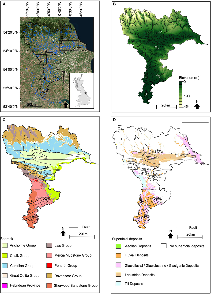
Figure 1. Locations and geological setting of the River Derwent Catchment; (A) Location of catchment. Including the sub-catchment locations for assessing macroinvertebrate data. Locations are shown; Pi, Pickering; M, Malton; Po, Pocklington; E, Elvington; B, Bubwith; and W, Wressel; (B) elevation variation within the catchment, locations shown; (C) bedrock geology and (D) superficial geology. Locations shown for B–D; Pi, Pickering; M, Malton; Po, Pocklington; E, Elvington; and B, Bubwith.
Erosion Risk Modeling
Erosion risk was modeled using the open-source plugin SCIMAP developed by the University of Durham (Lane et al., 2006, 2009; Reaney et al., 2011; Milledge et al., 2012) in ‘System for Automated Geoscientific Analyses’ (SAGA) GIS (Conrad et al., 2015). We modify the input data to SCIMAP in order to assess seasonality (in terms of rainfall and land use) and the impact of human influence on the catchment. Seasonality was tested in the year 2016 by assessing erosion risk for 1 month of the hydrological year; winter – February 2016; spring – April 2016; summer – July 2016; and autumn – November 2016. The months chosen were dictated by satellite imagery quality in relation to cloud coverage and are deemed representative of each season. SCIMAP requires the following datasets as inputs: DEM, precipitation data and land-use data. The DEM was downloaded from the Ordnance Survey (OS), in British National Grid co-ordinates and has a grid size of 5 m, and a vertical root mean square error of 1.5 m in urban areas and 2.5 m in rural, mountainous and moorland areas. The DEM was clipped to the study area, but no other processing was carried out, such as infilling the data gaps, as the SCIMAP plugin has this option. Rainfall data for the selected months were downloaded from the Met Office via the Centre for Environmental Data Analysis. The data grids, used in the UK Climate Projections 2009 (UKCP09) have a spatial resolution of 5 km. The monthly averages (total, mm) and long term averages (mm) data sets were downloaded, resampled to 5 m, and clipped to the study catchment.
SCIMAP produces a relative assessment of erosion risk across the catchment (a comparison of the riskiness of one location in a catchment compared to another location in a catchment), and does not produce absolute values (e.g., erosion in terms of tons ha–1); this is because the primary aim of erosion risk modeling is to identify the sources areas of sediment for management purposes. SCIMAP models erosion risk related to soil erosion, and associated in-channel risk, the methodology of this is explained below.
SCIMAP calculates erosion risk based on the energy available for erosion (hydrological risk) and the resistance to erosion (related to the potential for soil erosion), which is used to weight the hydrological risk (Reaney et al., 2011). The risk generation parameter in SCIMAP is a combination of these two parameters:
Where Pig is the risk generation parameter, Pih is the energy available to erode the material, and Pie is the risk of that material being eroded.
The energy available to erode the material (Pih) is represented as a stream power index related to the upstream contributing area, which determines the depth of water and soil erosion potential, and the local slope (Reaney et al., 2011), which is stored in the topographic data:
Where Ωi is the stream power index, Ai is the upstream contributing area and βi is the local slope.
The risk of the material being eroded (Pie) is a function of the land-cover, in which each land-cover category is assigned an erosion risk value. SCIMAP uses the following values: Agricultural land – 1; grasslands – 0.03 peat bogs – 0.05; Woodland – 0.05, Heathland – 0.05; urban/sub-urban – 0. The land use map is reclassified to these values in order to run the model. This part of the risk framework assumes that the erodibility of the material, as conditioned by the land cover, is the most important (rather than integrating soil or geological data) (Reaney et al., 2011).
Once the risk generation parameter has been assigned, SCIMAP assesses the likelihood of the eroded material reaching the channel network looking at the hydrological connection of the landscape as defined by the topographic wetness index:
Where k is the topographic wetness index, β represents the local slope and α represents the rainfall weighted upslope contributing area. The local slope data are determined by the topographic data, whilst the rainfall data are input in a raster format.
SCIMAP modifies the topographic wetness index, resulting in the network index (Reaney et al., 2011) as Walling et al. (2002) found only very small amounts of the total sediment mobilized are likely to reach the river channel. Therefore, less continuous hydrological flow pathways will result in more on-slope deposition. Therefore, the network index is based on the lowest value of topographic wetness index along a given flow path from the point of interest (source areas) to the drainage network (Lane et al., 2004). The network index combines topographic information (e.g., DEM) with rainfall data. Points with higher values of network index are more likely to be connected to the drainage net for a longer period of time. Only when there is a clear pathway for the sediment to enter the river network is risk considered. If there is erosion in part of the catchment that is not hydrologically connected to the river network, there will be no impact from the sediment production (Reaney et al., 2011).
SCIMAP finally routes and accumulates the risk through the channel network, and it is assumed the risk at a point is the sum of all location risk upstream of that point; this risk loading (the sum of the upstream risk) results in the in-channel risk concentration. The final stage of the SCIMAP framework does not take into account the loss of risk due to deposition or chemical transformations (Reaney et al., 2011). SCIMAP’s approach has been validated in a range of studies (e.g., Lane et al., 2006, 2009; Reaney et al., 2011) and is currently the main erosion risk tool used by stakeholders in the United Kingdom, such as the Environment Agency.
The erosion risk data presented here, which are related to the risk generation parameter and hydrological connectivity, range from 0 to 100%, and are shown where there is >50% erosion risk (e.g., the landscape unit has >50% likeliness to be contributing to diffuse pollution in the catchment). In order to compare the different model scenario outputs, the relative in-channel concentration (the risk loading) data were classified as: high risk >1.5 standard deviation; medium risk 0.83 – 1.5 standard deviation, low risk 0.17 – 0.83 standard deviation; and very low risk <0.17 standard deviation. Table 1 presents the datasets used within the erosion risk modeling undertaken in this paper.
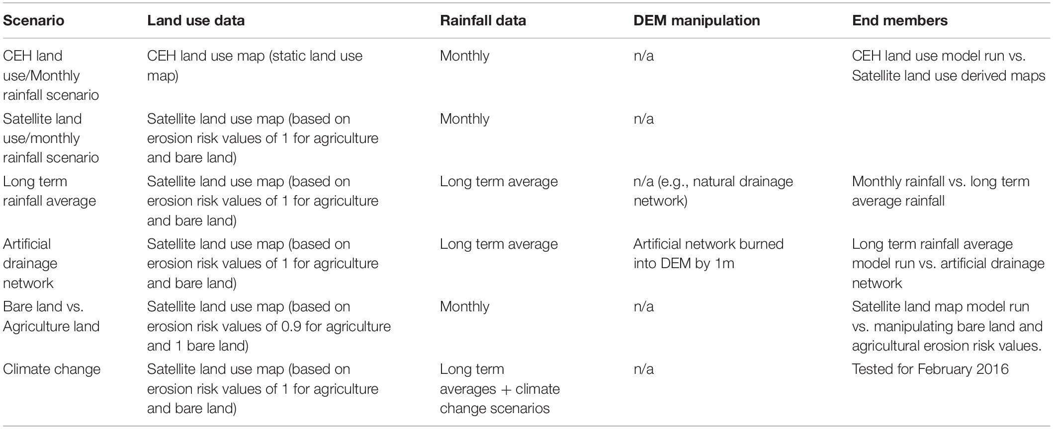
Table 1. Modeling scenarios and data used.
Land Use Data
Commonly, freely available datasets, such as the CORINE land use map or CEH (2015) land use maps, are used in erosion risk mapping. Although these are based on satellite imagery they do not show seasonal variation. Therefore, Sentinel 2 data, freely available from the European Space Agency (spatial resolution of 10 m) were downloaded (bands 2, 3, 4, and 8) and processed in SAGA GIS using image processing tools. Object-based image segmentation creates shapefile segments depending on the colors of the underlying image (e.g., similar greens will form a polygon). Once the image has segments, 50 segments for each land use type are ‘trained’ by assigning a land use classification. For this project, the following land-use classes were used, based on the CEH land use map: urban/sub-urban; peat bog; pastures; forest; agriculture; moors/heathland; and bare land. As this land use map was employed for erosion risk, the differentiation of different habitats, for example broadleaved forest versus conifer forest, was not required. Supervised classification for shapes is based on the information provided in training cells combined with the color combination of the underlying image. This tool produces a classified land use map for the whole catchment to which the SCIMAP landscape erosion values can be assigned.
Artificial Drainage
SCIMAP, like all GIS software, extracts the drainage network using the upstream contributing area. However, artificial drains/pathways are small features that are not picked up using the normal DEM and extracting processes. Due to the agricultural history of the Derwent Catchment, artificial drains (trellised drainage around field boundaries, Radcliffe et al., 2015) are common. Artificial drains, especially during high intensity rainfall events, can provide additional pathways for sediment to enter the drainage network, and therefore need to be incorporated into the modeling. Artificial drainage lines were downloaded as shapefiles from OS maps. These drainage lines were ‘burned’ into the DEM by 1 m using the ‘burn stream network into DEM’ tool in SAGA GIS (Conrad et al., 2015); this tool allows the DEM to be artificially deepened in these locations to ensure a flow path is created when the DEM is used in hydrological processing. The depth of the artificial drains is unknown, as they have not been surveyed, and higher resolution topographic information is not available; the 1 m depth is considered a conservative estimate in the absence of depth information.
Climate Change Data
Climate change data were downloaded from the Met Office, via the United Kingdom Climate projects website. The United Kingdom Climate Projections 2009 (UKCP09) cumulative distribution function (CDF) plots were used to change the long term average rainfall raster files downloaded from Centre for Environmental Data Analysis (CEDA), under different climate change forecasts. The month of February was chosen as a test, as climate predictions show wetter winters, until higher resolution UKCP18 data are released (which will be able to look at high intensity rainfall events in more detail). CDF plots for high, medium and low scenarios were looked at with the percent change in rainfall in the following quartiles recorded: Q10, Q50 and Q90; this provides a range of different climate scenarios that can be used to assess future sediment risk changes. Climate change scenarios were run for the years 2020–2049. CDF plots are split into 25 km2 squares. Therefore, the long term rainfall raster for February was clipped into the squares. Once a square of the raster was clipped, the percent change in rainfall due to a scenario (e.g., high emissions, Q10) was applied to the raster using the raster calculator. For example, if there was a 5.5% increase in rainfall, the raster calculator was used to increase the raster cell values by 5.5% (e.g., cell/100 ∗ 105.5). The new climate change rasters were then used in erosion risk mapping.
Model Runs and Assumptions
Erosion risk scenarios were run using the following assumptions and data (Table 1): (1) CEH land use maps (2015 version); (2) ‘seasonal’ satellite land use; (3) natural drainage; (4) artificial drainage; (5) current rainfall; (6) long term average rainfall; (7) land use risk between bare land and agriculture; and (8) projected climate change (for the month of February only). Running the model with different scenarios produces end members of erosion risk. This allows a range of outputs to be created to help understand the variation of erosion risk within the catchment.
Modifying the DEM by ‘burning’ the artificial drainage assumes: (1) that the field drains are hydrologically connected to the drainage network and will have flowing water during high flow conditions; (2) that the drains are not dredged by land owners; and (3) that the drains are roughly 1 m in depth (a value used in the absence of field data to verify drain depth). In previous studies of the Derwent catchment, field drains in the River Rye catchment were shown to be an important pathway for the transfer of sediment to the main river network (Sear, 1992). However, Newson (2006) concluded that the level of connectivity needs further investigation. Therefore, using the artificial network forms one end member of model runs. In order to understand variation between different scenario outputs, a DEM of difference was produced, which calculates the difference between two rasters by using the ‘minus’ tool in ArcGIS.
Morphometry
Morphometry is the quantification of catchments via indices such as river network analysis and stream profile analysis (Horton, 1932; Miller, 1953; Schumm, 1956; Chorley, 1957; Strahler, 1964). Morphometry can provide information on the history of a catchment, and current system dynamics, such as stream power. The normalized steepness index (KSN) quantifies the stream gradient, and is expected to be relatively consistent along a river course. Variation in the index is typically due to variation in tectonics or climate or lithology (Hack, 1973). The normalized steepness index was calculated using the topotoolbox plugin for Matlab (Schwanghart and Kuhn, 2010; Schwanghart and Scherler, 2014) and the equation is detailed below:
Where, KSN is the normalized steepness index, S is slope and θ is channel concavity.
Slope was extracted from the DEM using the slope toolbox in GIS. The slope tool calculates the maximum rate of change in value from that original cell to neighboring cells.
Sediment Sensitive Species
Understanding the impact of temporal variation in sediment concentration requires repeated sampling across the entire catchment, with samples taken across the entire range of hydrological flow conditions (Reaney et al., 2011). However, routine water quality sampling is rarely undertaken in catchments. In previous studies assessing erosion risk within catchments, results have been displayed in terms of impacts on salmonids (Reaney et al., 2011) and pearl mussels (Horton et al., 2015). Macroinvertebrates are reliable indicators of environmental conditions (Extence et al., 2013), and have been used to assess water quality in a range of locations (Armitage et al., 1983). One indicator is the Proportion of Sediment Sensitive Invertebrates (PSI; see Extence et al., 2013, for calculation), which looks at the invertebrate communities present to assess the influence of sediment (silt) on the channel bed. Briefly, the different species taxa present are assigned to one of four fine sediment-sensitivity ratings, due to their habitat preference (after extensive literature reviews and assessment of anatomical, physiological and behavioral traits of the species). The overall value is abundance weighted, showing the sensitivity of the whole population sample. PSI varies based on the species present, therefore it can be used to interpret the presence or absence of silt. PSI ranges from 0 (entirely silted bed) to 100 (unsilted bed) (Extence et al., 2013). Macroinvertebrate assemblages are routinely monitored under the Water Framework Directive (WFD) in the United Kingdom, within the Derwent catchment six sub-catchments (Figure 1A) were used to assess how helpful PSI is when trying to understand seasonal erosion risk using SCIMAP model outputs. Sediment sensitive invertebrate data were provided by the Environment Agency, who have processed the species present during the Spring and Autumn of 2016 through the PSI method (Extence et al., 2013) and provided a score between 0 and 100 for each site. These datasets combine the data collected during the routine WFD monitoring to produce an average value for the season for each site within the study areas. Within the six sub-catchments, a maximum of 22 sites and minimum of 1 site have fed into the PSI analysis (the spatial coverage of sites is related to WFD pressures in each sub-catchment).
Results
Catchment Morphometry
Figure 2A shows the slope of the River Derwent Catchment. Overall, the catchment has low slopes (<2°). Higher angled slopes can be found in the upland areas and North East areas of the catchment around Pocklington (>8°), and the upland headwater regions in the north of the catchment, north of Pickering (>25°). Normalized steepness index values (Figure 2B) are >18 in the upland areas, reflecting the higher slope values. The highest values (>50) can be found along the River Derwent and River Rye, upstream of their confluences. The middle reaches of the River Derwent are characterized by low slopes (<2°) and KSN values below 13, which are dominated by agricultural land use (Figures 2A,B).
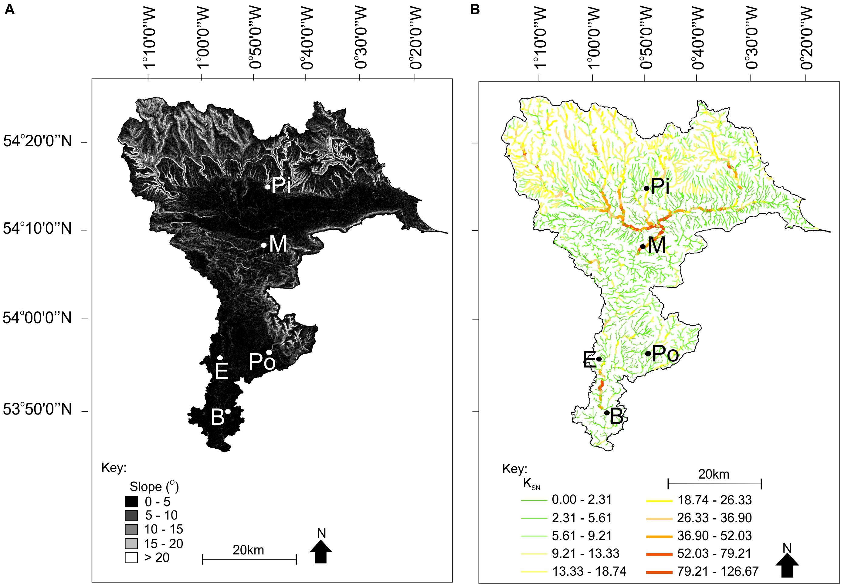
Figure 2. (A) Slope and (B) normalized steepness index of the River Derwent Catchment. Locations shown; Pi, Pickering; M, Malton; Po, Pocklington; E, Elvington; and B, Bubwith.
Erosion Risk Modeling: Scenario Outputs
Seasonal Variation
Erosion risk mapping scenarios for each season (Figures 3–6) show: (A) CEH land use map; (B) Satellite-derived land use map; (C) the DEM of difference between the two land use maps; (D) long term rainfall average; (E) monthly rainfall totals; (F) the DEM of difference between the two rainfall scenarios; and (G) the artificial drainage network.
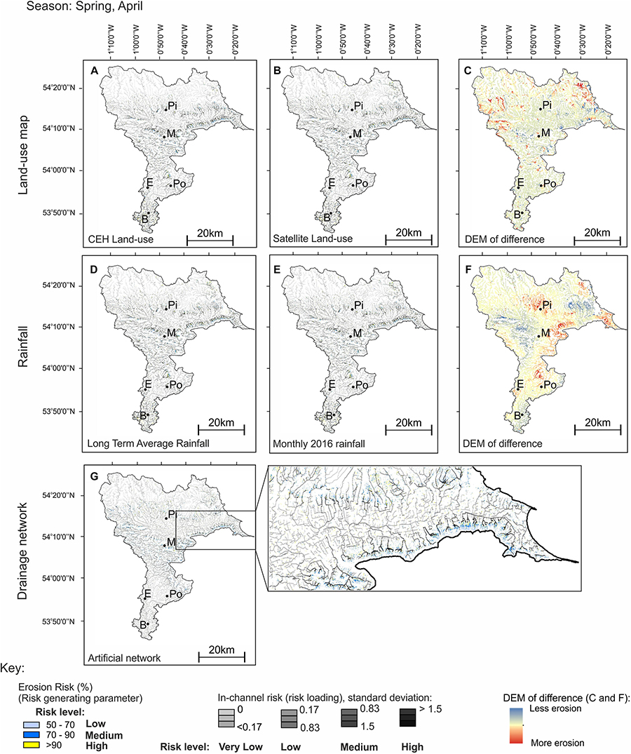
Figure 3. Model scenario outputs for April, (A) CEH land use map; (B) Satellite derived land use map; (C) the DEM of difference between the two land use maps; (D) Long term rainfall average; (E) monthly rainfall totals; (F) the DEM of difference between the two rainfall scenarios; and (G) the artificial drainage network. Locations are shown on each map; Pi, Pickering; M, Malton; Po, Pocklington; E, Elvington; B, Bubwith.
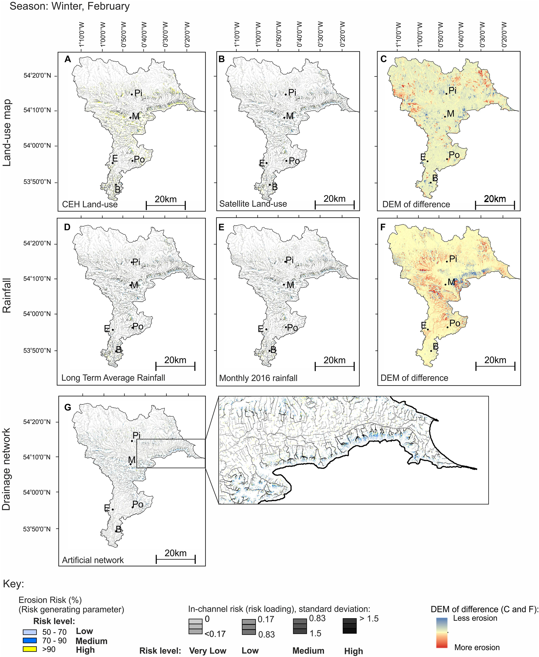
Figure 4. Model scenario outputs for February, (A) CEH land use map; (B) satellite-derived land use map; (C) the DEM of difference between the two land use maps; (D) long-term rainfall average; (E) monthly rainfall totals; (F) the DEM of difference between the two rainfall scenarios; and (G) the artificial drainage network. Locations are shown on each map; Pi, Pickering; M, Malton; Po, Pocklington; E, Elvington; B, Bubwith.
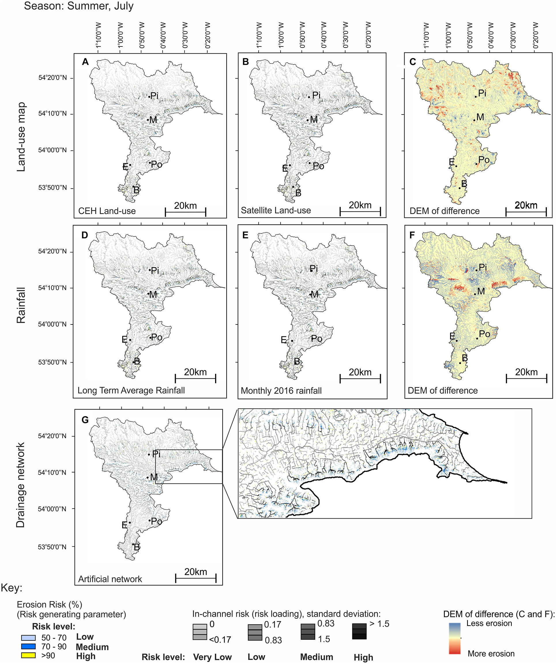
Figure 5. Model scenario outputs for July, (A) CEH land use map; (B) satellite-derived land use map; (C) the DEM of difference between the two land use maps; (D) long term rainfall average; (E) monthly rainfall totals; (F) the DEM of difference between the two rainfall scenarios; and (G) the artificial drainage network. Locations are shown on each map; Pi, Pickering; M, Malton; Po, Pocklington; E, Elvington; B, Bubwith.
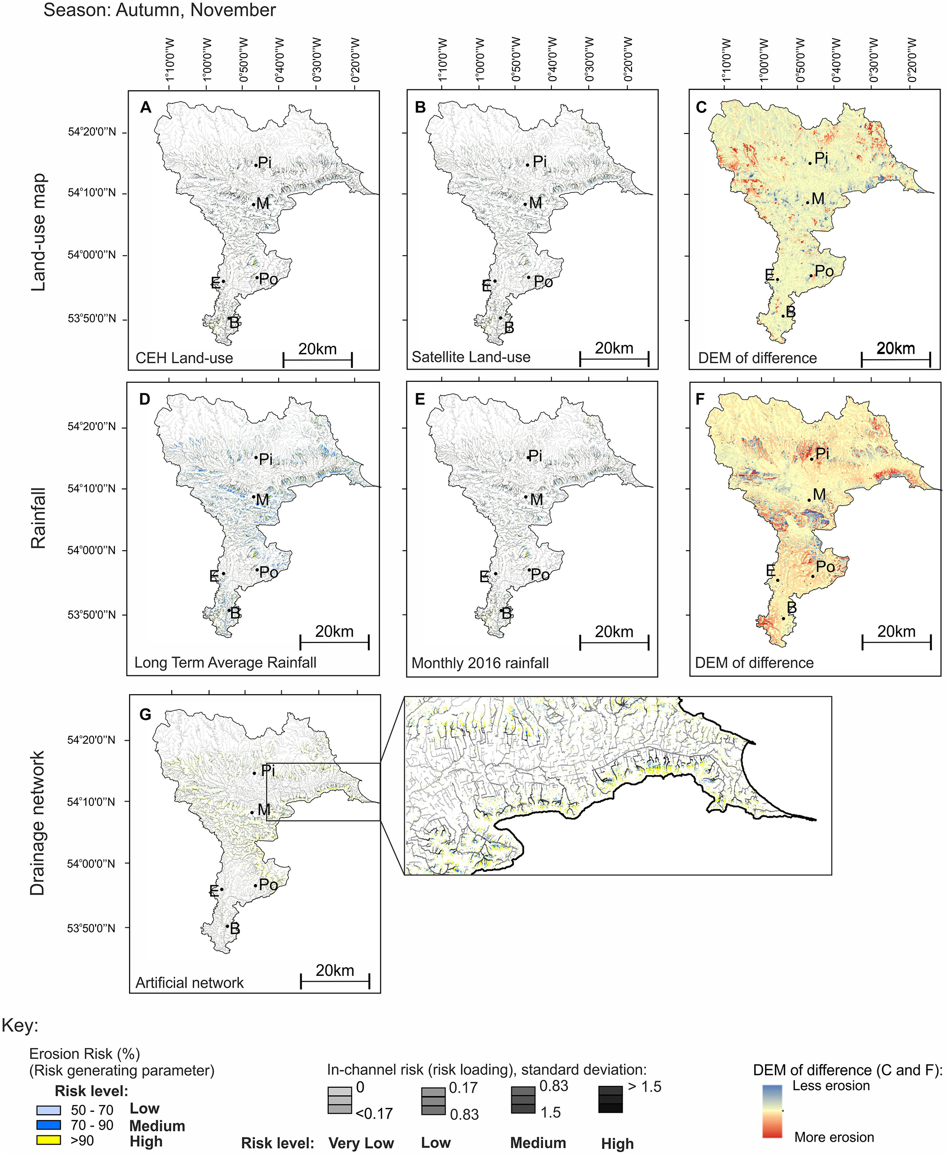
Figure 6. Model scenario outputs for November, (A) CEH land use map; (B) satellite-derived land use map; (C) the DEM of difference between the two land use maps; (D) long-term rainfall average; (E) monthly rainfall totals; (F) the DEM of difference between the two rainfall scenarios; and (G) the artificial drainage network. Locations are shown on each map; Pi, Pickering; M, Malton; Po, Pocklington; E, Elvington; B, Bubwith.
Overall, source areas of sediment are dominated by the agricultural lowland areas. The upland areas that comprise moorland and peatland had a relatively low risk of erosion through all of the modeling scenarios. Table 2 highlights the percentage of catchment coverage for each risk category between the scenarios tested, and offers a way to semi-quantify the modeling output as SCIMAP produces a relative assessment of erosion risk.
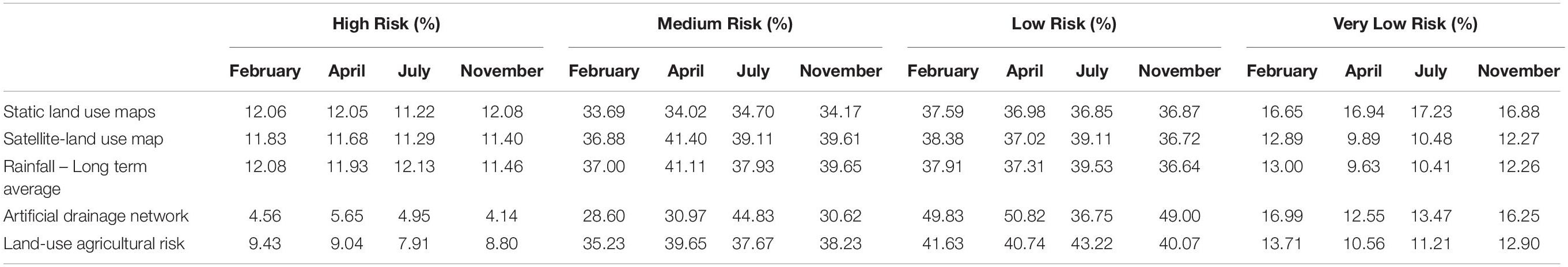
Table 2. Variation in categories of erosion risk (%) in different scenarios modeled (see Table 1 for end member comparisons and data used).
There are clear spatial trends in the yearly 2016 rainfall data (Figure 7). Maximum rainfall in February 2016 centered on the escarpment areas to the north east of the catchment and toward the mouth of the catchment. During July, rainfall rates are highest in the east of the catchment. However, in the upland area of the catchment there is not an associated increase in risk due to the land use cover (primarily peat/moorland). In November and April 2016, rainfall rates were lowest in the upland areas of the catchment and highest across the lowland areas. Overall, when using monthly rainfall values, April had more areas of high and medium risk within the catchment (52% coverage of the catchment area, Table 2), and February had more areas of low and very low risk (55% coverage of the catchment area, Table 2). When using the long term average rainfall data, April had more high and medium risk areas (53% coverage of the catchment area, Table 2), and February had more areas of low and very low risk (50% coverage of the catchment area, Table 2). In April, there is higher risk of erosion in the upland areas of the catchment, which is not seen during the other months modeled. Overall, when using the long term rainfall values, the DEM of difference highlights that the 2016 monthly values underestimate erosion risk, with the largest difference in February (Table 2).
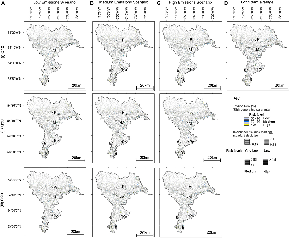
Figure 7. Seasonal variation in (A) erosion risk; (B) rainfall data and (C) bare land for 2016, for (i) winter; (ii) Spring; (iii) Summer; and (iv) Autumn. Location are shown on each map; Pi, Pickering; M, Malton; Po, Pocklington; E, Elvington; and B, Bubwith.
When modeling the difference in land use maps, the main critical source areas (high risk areas) have limited variation between the CEH- and satellite-derived land use maps (Figures 3–6), and are reasonably consistent seasonally, in which the lowland areas show greater levels of risk. When using both the CEH- and satellite-derived land use maps, erosion risk was highest in April. However, the satellite-derived land use maps had a greater coverage of high and medium risk areas (53% coverage of the catchment area, Table 2) compared to the CEH maps (46% coverage of the catchment area, Table 2). There is slightly less risk in the area around Pocklington in November compared to the other months modeled (Figure 6). Within each month modeled there are subtle differences between the CEH- and satellite-derived land use maps (when using the monthly rainfall values); as shown by the DEMs of difference (Figures 3C–6C). Typically, the CEH land use maps relatively underestimate the coverage of medium erosion risk across the catchment (by up to 6%, Table 2) and relatively overestimate areas of very low risk (by up to 7%, Table 2) when compared to the satellite-derived land use maps.
Erosion Modeling in Agriculture Dominated Catchments
Integrating the artificial drainage network only has an influence in the agricultural intensive areas, and no changes are seen in the upland areas of the catchment in erosion risk (Figures 3G–6G). By increasing the number of pathways there are more medium risk areas in the lowland regions of the Derwent catchment in July (45% coverage of the catchment area, Table 2). Overall, incorporating the artificial drainage increases the relative coverage of low risk areas in the lowland areas, across 3 of the 4 seasons modeled compared to the other scenarios modeled (Table 2).
Bare land changes seasonally within the Derwent Catchment due to cropping practices. The maximum bare land recorded is 18% (363 km2) of the catchment in February, reducing to 15% in April and February (314 km2) with the lowest coverage of bare land being 10% recorded in July (216 km2). When comparing agricultural land and bare land by manipulating the erosion risk values assigned to the land uses in SCIMAP there is a clear difference in erosion risk between each scenario (Figure 8). By integrating differences in erosion risk between bare land and agricultural land with crops visible on the satellite imagery, traditional erosion risk mapping that use the same value for all agricultural land regardless of cropping stage relatively overestimate high and medium risk areas by up to 5%, with the greatest variation in the month of July, with the highest risk in April in the River Derwent catchment.
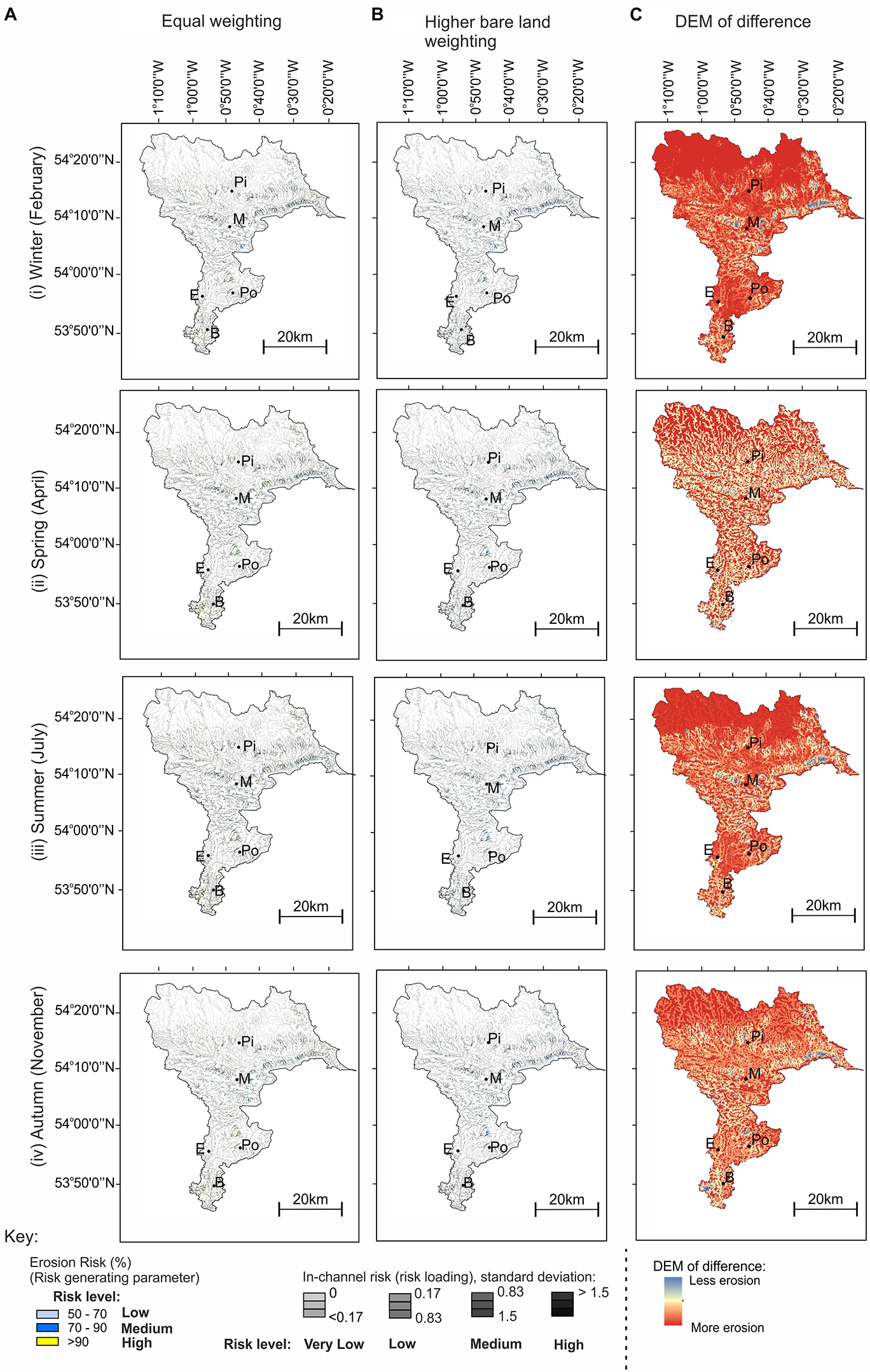
Figure 8. Model scenario showing change in erosion risk across the seasons: (i) Winter; (ii) Spring; (iii) summer; (iv) Autumn, when (A) agricultural land and bare land have the same erosion risk assigned; (B) when erosion risk in bare land is higher and (C) the DEM of difference. Locations are shown on each map; Pi, Pickering; M, Malton; Po, Pocklington; E, Elvington; B, Bubwith.
Future Climate Change
Figure 9 shows the impact of climate change under different climate projections (Low, Medium, and High); the source areas of sediment do not change regardless of the climate change scenario used. Under different climate change scenarios, source areas continue to be dominated by the lowland agricultural areas in the River Derwent catchment (assuming land use does not change).
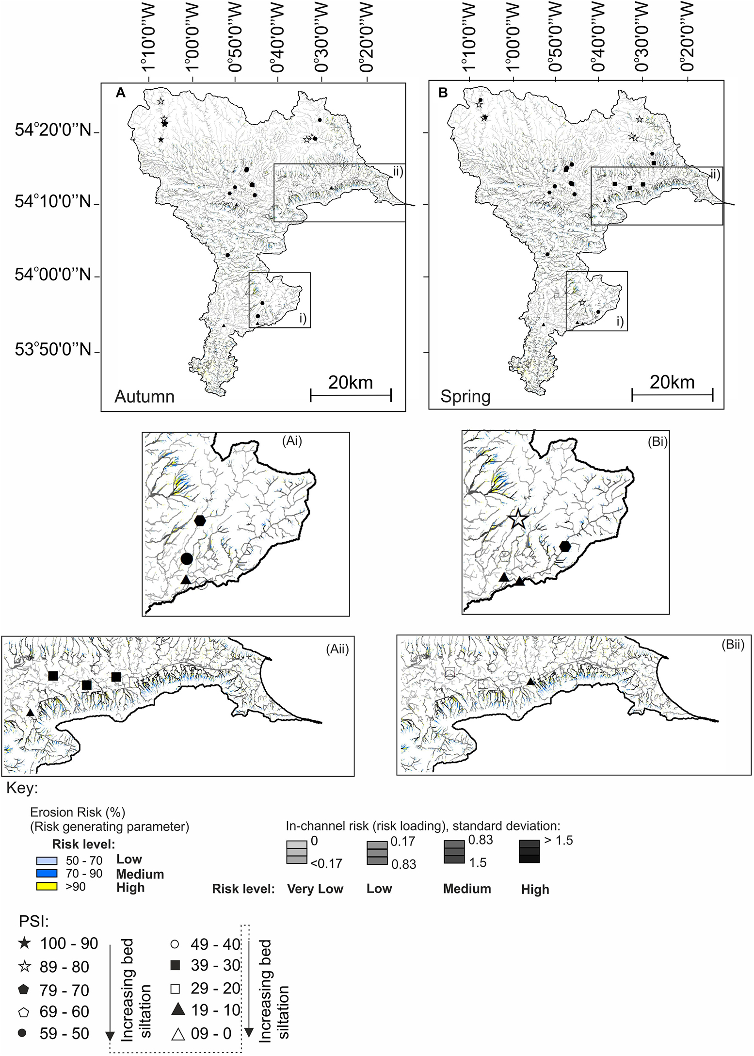
Figure 9. Model scenario outputs for climate change scenarios in February, depicting (A) Low, (B) medium and (C) high emission scenarios, for the following quartiles: (i) Q10; (ii) Q50 and (iii) Q90 using UCKCP09 data (D) the long term average. Locations are shown on each map; Pi, Pickering; M, Malton; Po, Pocklington; E, Elvington; B, Bubwith.
Sediment Sensitive Species
Figure 10 shows the portion of sediment sensitive species (%) within the Derwent catchment. Values vary seasonally within the catchment. The upper reaches of the catchment show high values of PSI (70+) within both spring (Figure 10A) and autumn (Figure 10B) indicating the bed is not affected by silt. However, PSI decreases downstream in the lowland area (0–50), which indicates there is increased silt deposition. Spring has more PSI values below 30 within the lowland areas of the catchment, which suggests higher levels of silt deposition (Figure 10A).
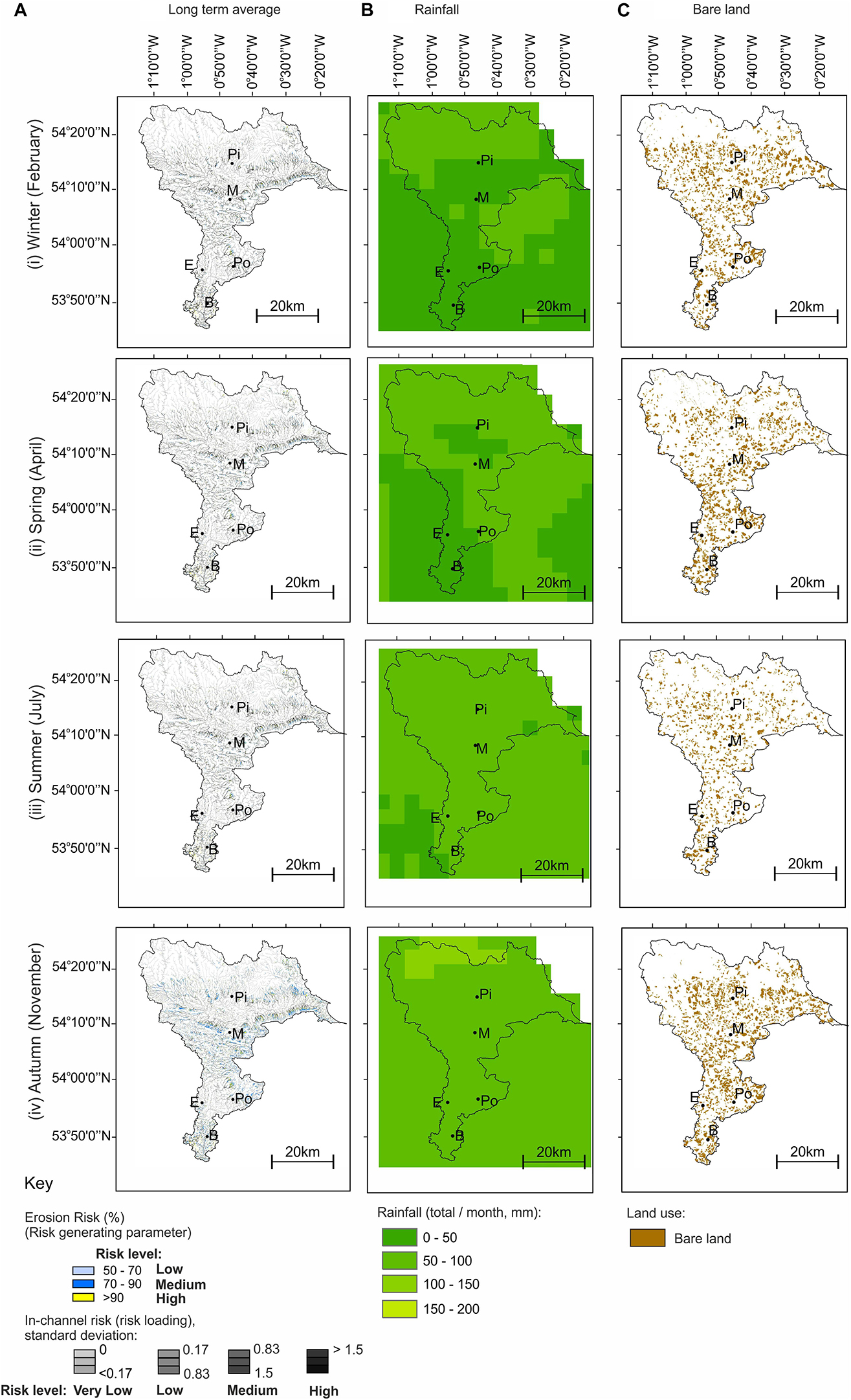
Figure 10. Variation in sediment sensitive species in (A) autumn and (B) spring across the year, the base maps show the erosion risk when using the long term average rainfall scenario (Table 2). Inserts show higher resolution study areas from (A,B). Locations are shown on each map; Pi, Pickering; M, Malton; Po, Pocklington; E, Elvington; B, Bubwith.
Discussion
Seasonal Variation
The purpose of this work is to show the importance of seasonal data when assessing erosion risk. The output modeling of SCIMAP requires validation in future work; results presented here therefore represent a relative assessment of different erosion models. Figures 3A-C–6A-C illustrate the importance of using seasonal land use maps, as the yearly averaged CEH maps relatively estimate 6% less erosion risk (Table 2 and Figures 3C–6C), although many of the critical source areas (high and medium risk) stay the same. Management may be targeted in the wrong areas and misuse limited resources due to the difference between yearly and seasonal estimations. Management based on the CEH land-use maps may not be in the most effective places or may prioritize the wrong areas. The variation is due to the data resolution (CEH is 1 km compared to 10 m for the satellite data). If smaller pockets of different land use can be identified using high resolution imagery, then more realistic land use maps can be produced that will improve modeling outputs. The variation in land use maps is exacerbated by the dominance of agriculture in the Derwent catchment, which is discussed in Section “Erosion Risk in Agricultural Dominated Catchments.” Land use types that can be modeled to reflect variations in plant coverage could also include areas of tree plantation, or areas affected by moorland fires. However, areas with relatively continuous cover, such as grasslands or peatlands, may not benefit from high risk modeling as there is limited seasonal variation. Nonetheless, by using high resolution satellite images the temporal and spatial variation in risk can be assessed more robustly as more detailed rainfall information can be used.
The spatial variation in rainfall across the catchment is compared to the seasonal bare land cover and erosion risk output (Figure 7). SCIMAP depicts relative risk within the catchment, and although the source areas are consistent, the volumes of sediment eroded and transported are expected to change due to variation in rainfall quantity and intensity. In 2016, November was the wettest month and had the largest percentage of bare land (18%), which would result in more sediment production. However, in November source areas around Pocklington have slightly less risk than the other months. This is possibly due to the spatial coverage of rainfall, resulting in a different configuration of connectivity between the source cells (land units), as defined by the network index. In alternative rainfall scenarios, different parts of the catchment may become activated, allowing seasonal variation in different flow pathways. April 2016 was also expected to produce high volumes of sediment due to the rainfall amounts and the second highest percentage of bare land. Figures 3D-F–6D-F show the variation in modeling when using the monthly and long term average rainfall values. Overall, the monthly 2016 rainfall values relatively underestimate erosion risk compared to the long term average rainfall, which is especially evident in February.
The modeling we present has compared the use of long term rainfall rates and monthly values, and seasonal land use maps, resulting in a range of scenarios. Erosion risk is an interlinked process, and risk based models relate this to land use and rainfall. Land use variation, especially in agricultural settings, is important to integrate. The percentage and location of bare land change seasonally; this could affect the pattern of source area cells and change connectivity. Seasonal variation in the intensity and location of rainfall will affect soil erosion, connectivity, and transport processes within the fluvial network. Producing a yearly average risk does not adequately show the complexity in risk that is experienced across the year. A scenario-based approach for erosion risk, using open access satellite imagery and rainfall data, allows multiple datasets and outcomes to be interrogated, and by integrating in seasonal variation help sediment management to become more strategic and resistant to future climate change. Catchments with clear variations in seasonal land coverage are particularly susceptible to poor management decisions using yearly average datasets. However, when mapping seasonality, caution must be taken to integrate both the monthly and long term averages of rainfall for each month. Management decisions based on an extreme monthly average (either high – a flood-prone year, or low – a drought year), could be flawed by placing management in areas that are not source areas each year. This would result in waste of resources, and could also negatively affect relationships with landowners who have set aside land.
Erosion Risk in Agricultural Dominated Catchments
Figures 3G–6G show the influence of using the artificial drainage network within the catchment. The sub-catchments dominated by agriculture and a higher coverage of field drains, such as the large lowland areas of the catchment, have increased area coverage of medium risk when incorporating the artificial network. Artificial networks should be incorporated in sub-catchments where there is a high coverage of field drains. Further investigation is required to assess if and when all drains are hydrologically connected, and these results represent one end member (fully connected 1 m deep field drains). Within erosion risk modeling, there is often an emphasis on gradient; high gradient areas cause greater risk and there is a greater coupling between source areas and the river channels (Hooke, 2003). However, within low gradient agricultural areas, sediment transport and overland flow has been recorded in tramlines that have increased connectivity within the catchment regardless of the low gradients. Recorded values of runoff have increased during a storm event from 0.4 to 8.4 mm due to creation of tramlines, resulting in increased sediment loads from 21 kg ha–1 to 400 kg ha–1 (Silgram et al., 2006).
By integrating the artificial drainage, the modeling is forced to recognize the additional pathways, and therefore represents the agricultural areas better. This work integrated artificial channels that were trellised around field boundaries. However, under-field drains also represent a key pathway (Radcliffe et al., 2015; Smith et al., 2015) that is often unmapped, whilst other water management practices such as irrigation can also increase erosion rates (Koluvek et al., 1993; García-Ruiz, 2010; Sojka, 2018).
The greatest seasonal variation in agricultural land is related to cropping cycles. Using satellite imagery not only increases the resolution of the data to 10 m, but seasonal maps are especially important in agriculturally dominated catchments where fields may be left bare seasonally (due to crop seeding or field rotation etc.), which increases erosion risk (Le Bissonnais et al., 2002). When assessing the erosion risk values assigned for SCIMAP, agricultural land is assumed to have the highest risk (of 1) regardless of the stage of cropping. However, the erosion risk associated with agricultural land can vary spatially and temporally due to multiple factors, such as the direction of contouring, crop types, crop growth stage, and management practices such as crop rotation (Heathwaite et al., 2005). When the crops are visible on satellite imagery, the erosion risk would be less than for bare land. By integrating land use maps developed from satellite imagery, bare land can be mapped and adequately included. Figure 8 shows the difference assigning bare land the highest erosion risk (1) and agricultural land, when the crop is visible (0.9), which more realistically represents erosion risk than assuming all agricultural land has the highest risk. By modeling the change in erosion risk due to the stage of agriculture development, satellite imagery can produce a more detailed assessment of erosion risk within a given year. In an agricultural setting, this is important as farmers may have to give up part of their land for sediment management, and by assessing when there is greatest risk, temporary measures could be implemented so that the land could be used for farming the rest of the year.
How Will Climate Change Affect Source Areas?
The source areas with the highest erosion risk (critical source areas) within the catchment do not change with different climate scenarios (Figure 9). This indicates that even with a maximum increase in rainfall using the high emission scenario, the areas of erosion risk will not change and there will be no new areas of sediment production. However, SCIMAP does not show erosion volumes, and the fact the source areas are the same does not indicate the amount of sediment produced will stay the same as erosion volumes are likely to increase due to higher quantities of rain providing more energy for geomorphic work (Burt et al., 2016). We used long term average rainfall data. However, geomorphic work is often carried out during high rainfall events, which have been shown to mobilize large volumes of sediment and cause increased risk (e.g., Mohamadi and Kavian, 2015; Marzen et al., 2017). Climate change scenarios suggest that high magnitude rainfall events are likely to become more frequent (e.g., Sarhadi and Soulis, 2017), and therefore mapping storm tracks and intensities could enable land managers to understand both the average and extreme events that contribute to the production and transport of sediment within a catchment. Incorporating climate change data into erosion risk studies is an essential future step to assess the longevity of management that can be proposed as well as future proofing the reduction in diffuse pollution.
Comparison of Data Output With Ecological Data
PSI, based on observed macroinvertebrate species data, has been shown to have a statistical relationship with sediment deposition (e.g., Glendell et al., 2014). Comparing PSI and erosion risk shows that the PSI is a good indicator of where sediment is deposited within the channel network (Figure 10). When assessing deposition from a geomorphological perspective, the PSI values can be used to infer geomorphological processes related to stream power variation which affect deposition, erosion and transportation within the network, which can be shown by KSN and surrounding slope values. When PSI values do not correspond to surrounding high levels of erosion risk in the Derwent as produced by SCIMAP, it shows that the channel in that location is efficient enough to transport sediment due to higher stream power. In some areas of low PSI scores (Figure 10Ai), the surrounding risk area is low. This indicates that sediment is sourced from upstream and that the river in the reach is not able to transport the sediment, either due to low stream power or the volume of sediment within the channel. Therefore, it is important to look upstream of the PSI location, as intervention in the immediate reach will not solve the local issues.
The upland areas of the catchment generally have low erosion risk and corresponding high PSI values (Figure 10). In these locations, the river is able to transport any suspended sediment that enters the drainage network. In agricultural areas, PSI decreases downstream indicating the buildup of sediment within the channel network (Figures 10Aii,Bii). In these locations, KSN and slope is low, indicating low rates of stream power. Some seasonal variation was shown in the PSI values in the agricultural areas, indicating that in spring the drainage network is not able to transport the sediment within the channel network. When looking at the long-term average rainfall rates, the highest erosion risk occurred within spring. However, the increase in discharge is balanced by the increase in erosion risk and therefore the overall channel capacity is reduced.
Incorporating further evidence, such as ecological data, is important in order to ground truth the erosion risk maps where detailed hydrological or hydraulic modeling cannot be carried out. Macroinvertebrate data can also focus where management should be placed. When incorporating these data it can be shown that the source areas for low PSI values are much further upstream and it would be more efficient to target those areas than the immediate surrounding area.
Causes of Erosion Risk
The Derwent catchment has a long history of natural and anthropogenic modification. In recent years, the channel has been straightened and deepened in several locations. The catchment is agriculturally intensive, and the seasonal variation in bare land and crops does impact the erosion risk within the catchment, as shown by using seasonal satellite imagery. The network of artificial field drains also increases connectivity by producing a complicated network of pathways.
The KSN shows that the main trunk of the River Derwent has a generally high capacity to transport sediment. However, fine grained sediment (clays, silts and fine grained sand) is stored in the system because of the volumes of sediment in the river, the lack of natural areas for the sediment to be deposited, the levees that keep flood waters contained, and the singular flow regime related to channel modification. This has caused high volumes of sediment to be processed at Elvington Treatment Works and has affected the designated sites in the lower Derwent.
The intensive agriculture, erodible soils due to geological history (Figure 1D) and management history has exacerbated the erosion regime within the River Derwent catchment. However, there is a lack of information on the catchment with regards to bank erosion that would be able to close the sediment budget. Due to the superficial deposits (Figure 1D), especially around Pickering, bank erosion is expected to be high. Bank erosion represents a key source of sediment within drainage networks, which is often exacerbated by animals entering the river course via the banks (poaching). A bank erosion study on the Rivers Swale, Ure and Ouse (the Derwent is a tributary of the River Ouse), Yorkshire, found average bank erosion between March 1996 and May 1997 to range from 77 to 440 mm (Lawler et al., 1999). Currently, there are no sediment budgets for the River Ouse that quantify the amount of sediment sourced from bank erosion relative to land use. Due to the erodible nature of the bedrock and superficial geology, bank erosion could represent a key sediment source in the Derwent catchment that needs to be monitored and integrated into further modeling.
Future Work and Wider Implications
Sediment concentrations naturally vary both spatially and temporally within river channels (e.g., Chakrapani, 2005). However, in the Derwent catchment as well as many other catchments modeled, there is no long term assessment of sediment concentrations. This is needed to assess how much of the present sediment problem is due to human modification in land use and channel management, or if a large portion is due to the erodible nature of the substrate that causes a ‘high’ natural base level. In order to inform policy and management of a catchment, the modern background sediment delivery needs to be understood, as well as historic rates which will give a more holistic approach to sediment management (Collins et al., 2011). Further, new climate change projections need to be integrated into modeling to forecast the future change in order to future proof any management or policies that are put in place. Additional data are needed to verify the model outputs, including identification of source areas in the field.
This paper has started to integrate seasonal variation in land-use and rainfall information into SCIMAP (Reaney et al., 2011) by varying the input data (land use maps and rainfall data). However, more in-depth seasonal modeling to look at different environmental scenarios needs to be undertaken using satellite imagery. Antecedent conditions such as the impact of a prolonged drought which could affect land-use (e.g., percent of bare land) or a high intensity localized storm event, which could increase hydrological connectivity, will impact and change diffuse pollution risk across the catchment. However, SCIMAP does not have a function to vary antecedent conditions for each model run. Because SCIMAP produces an erosion risk map for the length of data entered (e.g., monthly in this case), in order to understand the impact of a drought, preferably a daily time series (which will be affected by the satellite imagery temporal resolution related to the orbit of the satellites) would be needed to compare the output of a drought year to a ‘normal’ or wet year.
Future modeling should include bedrock/superficial geology and soil information (e.g., using RUSLE) in order to understand how much of the erosion is due to the erodible nature of the underlying geology. Land-use maps are a good proxy; incorporating additional information will give a greater confidence to erosion risk maps. Future modeling efforts should also incorporate high resolution information at field level, such as crop types and crop practices. Finally, in order to close the sediment budget the location and rate of bank erosion is vital to understand, as bank management as well as management of the landscape may be needed to reduce sediment loads within the river.
Additional information is required on the smaller pathways, which cannot be picked up using the 5 m DEM. High resolution reach-scale mapping should be used to investigate smaller pathways (e.g., rills within woodland areas). For the Derwent Catchment, these small pathways should be investigated on farmland and woodland areas. Furthermore, the depth and connectivity of the artificial channels need to be mapped during fieldwork, to allow correct manipulation of the DEM, rather than using a standard depth across the study area. Although a standard depth has been integrated for these model runs, it is not assumed that other depth values will significantly change the source areas; this is because when artificially modifying the DEM, flow is routed down these new channels. Nonetheless, deeper artificial channels will have the capacity to route higher sediment quantities and the areas of in-channel risk may vary; however, further work is needed to confirm this by collecting representative depths and re-running the models.
As well as impacting sediment volumes, anthropogenic activity impacts the ‘natural’ source to sink configuration (Figure 11) by accelerating pathways (e.g., artificial drainage), which is likely to be exacerbated by climate change increasing the volume of sediment produced (Burt et al., 2016). Although the delivery rate of sediment to the channel network has increased, additional stores, such as impoundments or natural flood management (e.g., earth bunds, buffer strips), may increase transport time to the sink (Figure 11). The movement of sediment through the channel network needs to be assessed to investigate lag times.
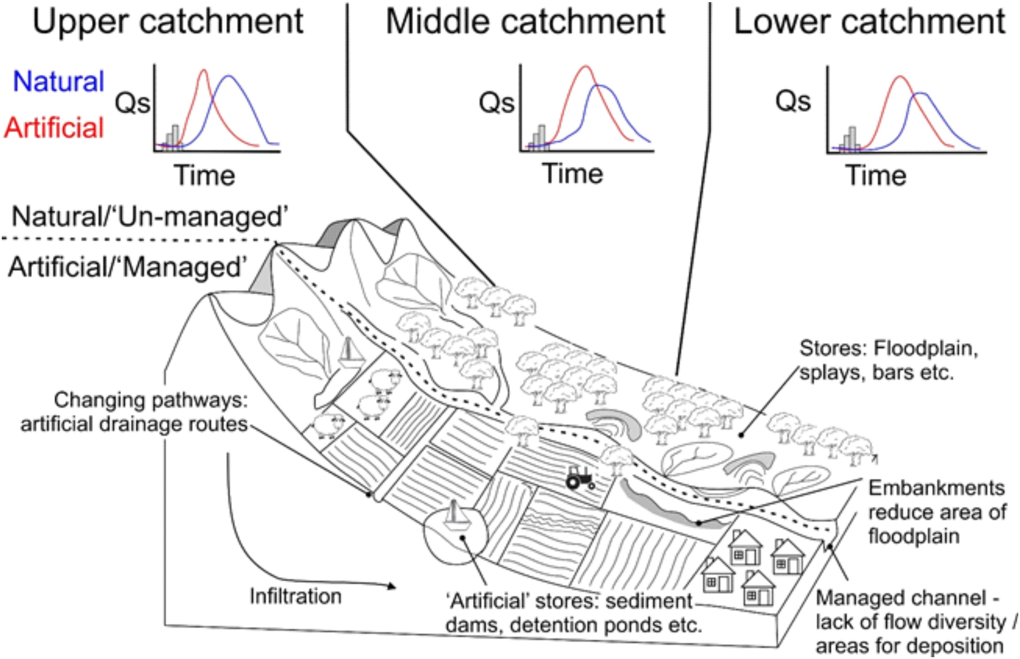
Figure 11. Synthesis figure showing the influence of anthropogenic (a ‘managed catchment’) activity on source to sink.
Rivers are a key transport route for pollutants and particulates, such as microplastics (e.g., Cole et al., 2011; Van Cauwenberghe et al., 2013; Lusher et al., 2015). However, there have been few studies linking source areas to the marine realm (e.g., Klein et al., 2015; Horton et al., 2017; Kane and Clare, 2019). Integrating high resolution modeling of source area erosion risk will allow a more holistic approach to be taken when assessing the dispersal of pollutants. This work has shown that seasonal variations in erosion risk is often relatively under-represented by modeling approaches. The seasonal variation in risk will translate to the flux of pollutants and particulates to the marine realm, which is an important aspect that needs to be integrated.
Conclusion
The Derwent catchment, Yorkshire, United Kingdom, illustrates how a scenario approach to erosion risk mapping can inform catchment management plans. By using seasonal land-use maps derived from open source satellite images and seasonal rainfall data, there is a clear variation in erosion risk both spatially and temporally. Typically, CEH land-use maps relatively underestimate erosion risk due to resolution issues and the static nature of the land-use map. Furthermore, in an agriculturally dominated catchment, artificial drainage should be incorporated, as this will overcome the natural bias to gradient in erosion risk mapping (e.g., steeper areas are of greater risk), as farming practices produce additional pathways that need to be considered. When using rainfall information, using the long term average for each month is recommended in order to remove the ‘extremes.’ However, future work should focus on using high resolution climate projections to assess the impact of localized high intensity rainfall events on erosion risk. For the Derwent catchment, this can be carried out when UKCP18 data are fully released. Further, the impact of drought or variation in other environmental conditions need to be integrated, and SCIMAP should be updated to integrate antecedent conditions.
In catchments dominated by agriculture, with large changes in seasonal land cover, a range of scenarios in erosion risk mapping is critical to improve management practices. Anthropogenic activity has changed the source-to-sink system. A holistic approach is needed to understand the new pathways and stores being created across the landscape to ensure that the ‘natural’ amount of particulates is transported through the system to reduce the risk of hungry water, and to forecast the flux of pollutants to the marine realm.
Data Availability Statement
The datasets generated for this study are available on request to the corresponding author.
Author Contributions
JR collected and analyzed the data, led the writing and drafting of figures, with major contributions on the text from DH and PK. DH helped to improve Figure 11. BA and AW supported JR throughout JRs NERC Industrial Mobility Fellowship and provided comments on the manuscript.
Funding
This work was funded under a NERC Industrial Mobility Fellowship to JR entitled ‘An Integrated Approach to Assessing Catchment Resilience: Combining GIS and Field Data in Relation To Climate Change Projections in the River Derwent’ (NERC Ref: NE/R013012/1). DH is funded under NERC Grant ‘Yorkshire iCASP – Yorkshire Integrated Catchment Solutions Programme’ (NERC Ref: NE/P011160/1).
Conflict of Interest
AW and BA are employed by Yorkshire Water.
The remaining authors declare that the research was conducted in the absence of any commercial or financial relationships that could be construed as a potential conflict of interest.
Acknowledgments
The Environment Agency Analysis and Reporting team for the Yorkshire Area and the Environment Agency catchment co-ordinator are thanked for their help during JRs NERC Industrial Mobility Fellowship and for providing ecological data on sediment sensitive species. We acknowledge the reviews by the three reviewers who helped to improve this manuscript.
References
Armitage, P. D., Moss, D., Wright, J. F., and Furse, M. T. (1983). The performance of a new biological water quality score system based on macroinvertebrates over a wide range of unpolluted running-water sites. Water Res. 17, 333–347. doi: 10.1016/0043-1354(83)90188-4
Ballantine, D. J., Walling, D. E., Collins, A. L., and Leeks, G. J. L. (2009). The content and storage of phosphorus in fine-grained channel bed sediment in contrasting lowland agricultural catchments in the UK. Geoderma 151, 141–149. doi: 10.1016/j.geoderma.2009.03.021
Bilotta, G. S., and Brazier, R. E. (2008). Understanding the influence of suspended solids on water quality and aquatic biota. Water Res. 42, 2849–2861. doi: 10.1016/j.watres.2008.03.018
Boggs, G., Devonport, C., Evans, K., and Puig, P. (2001). GIS-based rapid assessment of erosion risk in a small catchment in the wet/dry tropics of Australia. Land Degrad. Dev. 12, 417–434. doi: 10.1002/ldr.457
Bracken, L. J., Turnbull, L., Wainwright, J., and Bogaart, P. (2015). Sediment connectivity: a framework for understanding sediment transfer at multiple scales. Earth Surf. Process. Landf. 40, 177–188. doi: 10.1002/esp.3635
Bryan, R. B. (2000). Soil erodibility and processes of water erosion on hillslope. Geomorphology 32, 385–415. doi: 10.1016/S0169-555X(99)00105-1
Burt, T., Boardman, J., Foster, I., and Howden, N. (2016). More rain, less soil: long-term changes in rainfall intensity with climate change. Earth Surf. Process. Landf. 41, 563–566. doi: 10.1002/esp.3868
Cavalli, M., Trevisani, S., Comiti, F., and Marchi, L. (2013). Geomorphometric assessment of spatial sediment connectivity in small Alpine catchments. Geomorphology 188, 31–41. doi: 10.1016/j.geomorph.2012.05.007
Cerdan, O., Govers, G., Le Bissonnais, Y., Van Oost, K., Poesen, J., Saby, N., et al. (2010). Rates and spatial variations of soil erosion in Europe: a study based on erosion plot data. Geomorphology 122, 167–177. doi: 10.1016/j.geomorph.2010.06.011
Chakrapani, G. J. (2005). Factors controlling variations in river sediment loads. Curr. Sci. 88, 569–575.
Cole, M., Lindeque, P., Halsband, C., and Galloway, T. S. (2011). Microplastics as contaminants in the marine environment: a review. Mar. Pollut. Bull. 62, 2588–2597. doi: 10.1016/j.marpolbul.2011.09.025
Collins, A. L., Naden, P. S., Sear, D. A., Jones, J. I., Foster, I. D., and Morrow, K. (2011). Sediment targets for informing river catchment management: international experience and prospects. Hydrol. Process. 25, 2112–2129. doi: 10.1002/hyp.7965
Collins, A. L., Walling, D. E., and Leeks, G. J. L. (2005). “Storage of fine-grained sediment and associated contaminants within the channels of lowland permeable catchments in the UK,” in Proceedings of the Sediment Budgets 1 Symposium S1 Held During the Seventh IAHS Scientific Assembly at Foz do Iguaçu, (Wallingford, UK: IAHS Press), 259–268.
Conrad, O., Bechtel, B., Bock, M., Dietrich, H., Fischer, E., Gerlitz, L., et al. (2015). System for automated geoscientific analyses (SAGA) v. 2.1.4. Geosci. Model Dev. 8, 1991–2007. doi: 10.5194/gmd-8-1991-2015
Coulthard, T. J., Ramirez, J., Fowler, H. J., and Glenis, V. (2012). Using the UKCP09 probabilistc scenarios to model the amplified impact of climate change on drainage basin sediment yield. Hydrol. Earth Syst. Sci. 16, 4401–4416. doi: 10.5194/hess-16-4401-2012
Covich, A. P., Austen, M. C., Bärlocher, F., Chauvet, E., Cardinale, B. J., Biles, C. L., et al. (2004). The role of biodiversity in the functioning of freshwater and marine benthic ecosystems. Bioscience 54, 767–775.
Dampney, P., Mason, P., Goodlass, G., and Hillman, J. (2002). Methods and Measures To Minimise the Diffuse Pollution of Water From Agriculture–a Critical Appraisal. Report for Defra project NT2507. London.
Dietrich, W. E., and Dunne, T. (1978). Sediment budget for a small catchment in a mountainous terrain. Z. Geomorphol. Suppl. 29, 191–206.
Extence, C. A., Chadd, R. P., England, J., Dunbar, M. J., Wood, P. J., and Taylor, E. D. (2013). The assessment of fine sediment accumulation in rivers using macro-invertebrate community response. River Res. Appl. 29, 17–55. doi: 10.1002/rra.1569
Farnsworth, K. L., and Milliman, J. D. (2003). Effects of climatic and anthropogenic change on small mountainous rivers: the Salinas River example. Glob. Planet. Chang. 39, 53–64. doi: 10.1016/S0921-8181(03)00017-1
Fryirs, K. (2013). (Dis) Connectivity in catchment sediment cascades: a fresh look at the sediment delivery problem. Earth Surf. Process. Landf. 38, 30–46. doi: 10.1002/esp.3242
García-Ruiz, J. M. (2010). The effects of land uses on soil erosion in Spain: a review. Catena 81, 1–11. doi: 10.1016/j.catena.2010.01.001
Gitas, I. Z., Douros, K., Minakou, C., Silleos, G. N., and Karydas, C. G. (2009). Multi-temporal soil erosion risk assessment in N. Chalkidiki using a modified USLE raster model. EARSeL eProceedings 8, 40–52.
Glendell, M., Extence, C., Chadd, R., and Brazier, R. E. (2014). Testing the pressure-specific invertebrate index (PSI) as a tool for determining ecologically relevant targets for reducing sedimentation in streams. Freshwater Biol. 59, 353–367. doi: 10.1111/fwb.12269
Greig, S. M., Sear, D. A., Carling, P. A., and Whitcombe, L. (2005). Fine sediment accumulation in salmon spawning gravels and the survival of incubating salmon progeny: implications for spawning habitat management. Sci. Total Environ. 344, 241–258.
Hack, J. T. (1973). Stream-profile analysis and stream-gradient index. J. Res. U.S. Geol. Sur. 1, 421–429.
Heathwaite, A. L. (2003). Making process-based knowledge useable at the operational level: a framework for modelling diffuse pollution from agricultural land. Environ. Modell. Soft. 18, 753–760.
Heathwaite, A. L., Fraser, A. I., Johnes, P. J., Hutchins, M., Lord, E., and Butterfield, D. (2003a). The phosphorus indicators tool: a simple model of diffuse P loss from agricultural land to water. Soil Use Manage. 19, 1–11.
Heathwaite, A. L., Sharpley, A. N., Beckmann, M., and Rekolainen, S. (2003b). “Assessing the risk of agricultural nonpoint source phosphorus pollution,” in Phosphorus: Agriculture and the Environment, eds J. T. Sims and A. N. Sharpley (United Kingdom: ASA).
Heathwaite, A. L., Quinn, P. F., and Hewett, C. J. M. (2005). Modelling and managing critical source areas of diffuse pollution from agricultural land using flow connectivity simulation. J. Hydrol. 304, 446–461. doi: 10.1016/j.jhydrol.2004.07.043
Heckmann, T., Haas, F., Abel, J., Rimböck, A., and Becht, M. (2017). Feeding the hungry river: fluvial morphodynamics and the entrainment of artificially inserted sediment at the dammed river Isar, Eastern Alps, Germany. Geomorphology 291, 128–142. doi: 10.1016/j.geomorph.2017.01.025
Hodgson, D. M., Bernhardt, A., Clare, M. A., Da Silva, A. C., Fosdick, J., Mauz, B., et al. (2018). Grand challenges (and great opportunities) in sedimentology, stratigraphy, and diagenesis research. Front. Earth Sci. 6:173. doi: 10.3389/feart.2018.00173
Holmes, T. P. (1988). The offsite impact of soil erosion on the water treatment industry. Land Econ. 64, 356–366.
Hooke, J. M. (2003). Coarse sediment connectivity in river channel systems: a conceptual framework and methodology. Geomorphology 56, 79–94. doi: 10.1016/s0169-555x(03)00047-3
Horton, A. A., Svendsen, C., Williams, R. J., Spurgeon, D. J., and Lahive, E. (2017). Large microplastic particles in sediments of tributaries of the River Thames, UK–Abundance, sources and methods for effective quantification. Mar. Pollut. Bull. 114, 218–226. doi: 10.1016/j.marpolbul.2016.09.004
Horton, M., Keys, A., Kirkwood, L., Mitchell, F., Kyle, R., and Roberts, D. (2015). Sustainable catchment restoration for reintroduction of captive bred freshwater pearl mussels Margaritifera margaritifera. Limnologica 50, 21–28. doi: 10.1016/j.limno.2014.11.003
Huang, C., Gascuel-Odoux, C., and Cros-Cayot, S. (2002). Hillslope topographic and hydrologic effects on overland flow and erosion. Catena 46, 177–188. doi: 10.1016/S0341-8162(01)00165-5
Jordan, C., and Smith, R. V. (2005). Methods to predict the agricultural contribution to catchment nitrate loads: designation of nitrate vulnerable zones in Northern Ireland. J. Hydrol. 304, 316–329.
Kane, I. A., and Clare, M. (2019). Dispersion, accumulation and the ultimate fate of microplastics in deep-marine environments: a review and future directions. Front. Earth. Sci. 7:80. doi: 10.3389/feart.2019.00080
Klein, S., Worch, E., and Knepper, T. P. (2015). Occurrence and spatial distribution of microplastics in river shore sediments of the Rhine-Main area in Germany. Environ. Sci. Tech. 49, 6070–6076. doi: 10.1021/acs.est.5b00492
Koluvek, P. K., Tanji, K. K., and Trout, T. J. (1993). Overview of soil erosion from irrigation. J. Irrig. Drain. Eng. 119, 929–946. doi: 10.1061/(ASCE)0733-94371993119:6(929)
Kondolf, G. M., Gao, Y., Annandale, G. W., Morris, G. L., Jiang, E., Zhang, J., et al. (2014). Sustainable sediment management in reservoirs and regulated rivers: experiences from five continents. Earth’s Future 2, 256–280.
Köthe, H. (2003). Existing sediment management guidelines: an overview. J. Soils Sediments 3, 139–143.
Kronvang, B., Laubel, A., Larsen, S. E., and Friberg, N. (2003). Pesticides and heavy metals in Danish streambed sediment. Hydrobiologia 494, 93–101.
Lane, S. N. (2003). “More floods, less rain: changing hydrology in a Yorkshire context,” in Global Warming in a Yorkshire Context, ed. M. Atherden (York: Place Research Centre), 18–19.
Lane, S. N., Brookes, C. J., Kirkby, M. J., and Holden, J. (2004). A network-index-based version of TOPMODEL for use with high-resolution digital topographic data. Hydrol. Proc. 18, 191–201. doi: 10.1002/hyp.5208
Lane, S. N., Brookes, C. J., Louise Heathwaite, A., and Reaney, S. (2006). Surveillant science: challenges for the management of rural environments emerging from the new generation diffuse pollution models. J. Agric. Econ. 57, 239–257. doi: 10.1111/j.1477-9552.2006.00050.x
Lane, S. N., Reaney, S. M., and Heathwaite, A. L. (2009). Representation of landscape hydrological connectivity using a topographically driven surface flow index. Water Resour. Res. 45, doi: 10.1029/2008WR007336
Lawler, D. M., Grove, J. R., Couperthwaite, J. S., and Leeks, G. J. L. (1999). Downstream change in river bank erosion rates in the Swale–Ouse system, northern England. Hydrol. Proc. 13, 977–992. doi: 10.1002/(sici)1099-1085(199905)13:7<977::aid-hyp785>3.3.co;2-x
Le Bissonnais, Y., Montier, C., Jamagne, M., Daroussin, J., and King, D. (2002). Mapping erosion risk for cultivated soil in France. Catena 46, 207–220. doi: 10.1016/S0341-8162(01)00167-9
Liu, Q. Q., and Singh, V. P. (2004). Effect of microtopography, slope length and gradient, and vegetative cover on overland flow through simulation. J. Hydrol. En. 9, 375–382. doi: 10.1061/(ASCE)1084-069920049:5(375)
Lu, D., Li, G., Valladares, G. S., and Batistella, M. (2004). Mapping soil erosion risk in Rondonia, Brazilian Amazonia: using RUSLE, remote sensing and GIS. Land Degrad. Dev. 15, 499–512. doi: 10.1002/ldr.634
Lusher, A. L., Tirelli, V., O’Connor, I., and Officer, R. (2015). Microplastics in Arctic polar waters: the first reported values of particles in surface and sub-surface samples. Sci. Rep. 5:14947. doi: 10.1038/srep14947
Marzen, M., Iserloh, T., de Lima, J. L., Fister, W., and Ries, J. B. (2017). Impact of severe rain storms on soil erosion: experimental evaluation of wind-driven rain and its implications for natural hazard management. Sci. Total Environ. 590, 502–513. doi: 10.1016/j.scitotenv.2017.02.190
Mertes, L. A. (2002). Remote sensing of riverine landscapes. Freshwater Biol. 47, 799–816. doi: 10.1046/j.1365-2427.2002.00909.x
Milledge, D. G., Lane, S. N., Heathwaite, A. L., and Reaney, S. M. (2012). A Monte Carlo approach to the inverse problem of diffuse pollution risk in agricultural catchments. Sci. Total Environ. 433, 434–449. doi: 10.1016/j.scitotenv.2012.06.047
Miller, V. C. (1953). A Quantitative Geomorphic Study of Drainage Basin Characteristics in the Clinch Mountain Area. Virginia and Tennessee, Project. NR, Technical Report, Columbia University, New York, NY 389–402.
Mohamadi, M. A., and Kavian, A. (2015). Effects of rainfall patterns on runoff and soil erosion in field plots. Int. Soil Water Conserv. Res. 3, 273–281. doi: 10.1016/j.iswcr.2015.10.001
Mossa, J. (1996). Sediment dynamics in the lowermost Mississippi River. Eng. Geol. 45, 457–479. doi: 10.1016/S0013-7952(96)00026-9
Munafo, M., Cecchi, G., Baiocco, F., and Mancini, L. (2005). River pollution from nonpoint sources: a new simplified method of assessment. J. Environ. Manage. 77, 93–98.
Natural England, (2015). Pollution Risk Assessment and Source Apportionment: River Derwent Catchment. York: Natural England.
Newson, M. D. (2006). Desk-based Targeting for a Fluvial Audit of the Yorkshire River Derwent. Report on Contract 13691, Environment Agency North-east Region, York.
Orr, H. G., and Carling, P. A. (2006). Hydro-climatic and land use changes in the River Lune catchment, North West England, implications for catchment management. River Res. Appl. 22, 239–255. doi: 10.1002/rra.908
Owens, P. N., Batalla, R. J., Collins, A. J., Gomez, B., Hicks, D. M., Horowitz, A. J., et al. (2005). Fine-grained sediment in river systems: environmental significance and management issues. River Res. Appl. 21, 693–717. doi: 10.1002/rra.878
Panagos, P., Christos, K., Cristiano, B., and Ioannis, G. (2014). Seasonal monitoring of soil erosion at regional scale: an application of the G2 model in Crete focusing on agricultural land uses. Int. J. Appl. Earth Obs. Geoinfo. 27, 147–155. doi: 10.1016/j.jag.2013.09.012
Radcliffe, D. E., Reid, D. K., Blombäck, K., Bolster, C. H., Collick, A. S., Easton, Z. M., et al. (2015). Applicability of models to predict phosphorus losses in drained fields: a review. J. Environ. Qual. 44, 614–628. doi: 10.2134/jeq2014.05.0220
Reaney, S. M., Lane, S. N., Heathwaite, A. L., and Dugdale, L. J. (2011). Risk-based modelling of diffuse land use impacts from rural landscapes upon salmonid fry abundance. Ecol. Model. 222, 1016–1029. doi: 10.1016/j.ecolmodel.2010.08.022
Rickson, R. J. (2014). Can control of soil erosion mitigate water pollution by sediments? Sci. Total Environ. 468, 1187–1197. doi: 10.1016/j.scitotenv.2013.05.057
Royal Haskoning, (2010). Restoring the Yorkshire Derwent: River Restoration Plan. Amersfoort: Royal Haskoning.
Sarhadi, A., and Soulis, E. D. (2017). Time-varying extreme rainfall intensity-duration-frequency curves in a changing climate. Geophy. Res. Lett. 44, 2454–2463. doi: 10.1002/2016GL072201
Schumm, S. A. (1956). Evolution of drainage systems and slopes in badlands at Perth Amboy. New Jersey. Geol. Soc. Am. Bull. 67, 597–646.
Schwanghart, W., and Kuhn, N. J. (2010). TopoToolbox: a set of Matlab functions for topographic analysis. Environ. Model. Softw. 25, 770–781. doi: 10.1016/j.envsoft.2009.12.002
Schwanghart, W., and Scherler, D. (2014). TopoToolbox 2 – MATLAB-based software for topographic analysis and modeling in Earth surface sciences. Earth Surf. Dyn. 2, 1–7. doi: 10.5194/esurf-2-1-2014
Sear, D. A. (1992). Siltation at the confluence of the River Derwent and River Rye, North Yorkshire. Report to Yorkshire NRA Flood Defence Function, University of Newcastleupon-Tyne.
Silgram, M., Jackson, B., Quinton, J., and Stevens, C. (2006). “Practical mitigation options for controlling phosphorus and sediment loss at hillslope scale,” in Proceedings of the British Hydrological Society, 9th National Hydrology Symposium, (Durham).
Smith, D. R., King, K. W., Johnson, L., Francesconi, W., Richards, P., Baker, D., et al. (2015). Surface runoff and tile drainage transport of phosphorus in the midwestern United States. J. Environ. Qual. 44, 495–502. doi: 10.2134/jeq2014.04.0176
Sojka, R. E. (2018). “Understanding and managing irrigation-induced erosion,” in Advances in Soil and Water Conservation, ed. F. J. Pierce (Abingdon: Routledge), 21–37.
Strahler, A. N. (1964). “Quantitative geomorphology of drainage basins and channel networks,” in Handbook of Applied Hydrology, ed. V. T. Chow (New York, NY: McGraw Hill Book Company), 39–76.
Sustainable Futures (2018). Walk The Supply Chain, Yorkshire Water at Elvington Water Treatment Works. Available at: https://www.sustainablefutures.uk.com/walk-the-supply-chain/walk-supply-chain-yorkshire-water-elvington-water-treatment-works/ (accessed January 2019).
Syvitski, J. P., and Kettner, A. (2011). Sediment flux and the anthropocene. Philosophi. Transac. Royal Soc. A. 369, 957–975. doi: 10.1098/rsta.2010.0329
Syvitski, J. P., Vörösmarty, C. J., Kettner, A. J., and Green, P. (2005). Impact of humans on the flux of terrestrial sediment to the global coastal ocean. Science 308, 376–380. doi: 10.1126/science.1109454
Tucker, G. E. (2004). Drainage basin sensitivity to tectonic and climatic forcing: implications of a stochastic model for the role of entrainment and erosion thresholds. Earth Surf. Process. Landf. 29, 185–205. doi: 10.1002/esp.1020
Van Cauwenberghe, L., Vanreusel, A., Mees, J., and Janssen, C. R. (2013). Microplastic pollution in deep-sea sediments. Environ. Pollut. 182, 495–499. doi: 10.1016/j.envpol.2013.08.013
Van Sickle, J., and Paulsen, S. G. (2008). Assessing the attributable risks, relative risks, and regional extents of aquatic stressors. J. N. Am. Benthol. Soc. 27, 920–931. doi: 10.1899/07-152.1
Vrieling, A., De Jong, S. M., Sterk, G., and Rodrigues, S. C. (2008). Timing of erosion and satellite data: a multi-resolution approach to soil erosion risk mapping. Int. J. Appl. Earth Obs. Geoinf. 10, 267–281. doi: 10.1016/j.jag.2007.10.009
Walling, D. E. (2006). Human impact on land–ocean sediment transfer by the world’s rivers. Geomorphology 79, 192–216. doi: 10.1016/j.geomorph.2006.06.019
Walling, D. E., and Fang, D. (2003). Recent trends in the suspended sediment loads of the world’s rivers. Glob. Planet. Chang. 39, 111–126. doi: 10.1016/S0921-8181(03)00020-1
Walling, D. E., Owens, P. N., Waterfall, B. D., Leeks, G. J., and Wass, P. D. (2000). The particle size characteristics of fluvial suspended sediment in the Humber and Tweed catchments, UK. Sci. Total Environ. 251, 205–222. doi: 10.1016/S0048-9697(00)00384-3
Walling, D., Russell, M., and Hodkinson, R. (2002). Establishing sediment budgets for two small lowland agricultural catchments in the UK. Catena 47, 323–353. doi: 10.1016/s0341-8162(01)00187-4
Wilkinson, B. H., and McElroy, B. J. (2007). The impact of humans on continental erosion and sedimentation. Geol. Soc. Am. Bull. 119, 140–156. doi: 10.1130/B25899.1
Wilkinson, S. N., Prosser, I. P., Rustomji, P., and Read, A. M. (2009). Modelling and testing spatially distributed sediment budgets to relate erosion processes to sediment yields. Environ. Model. Softw. 24, 489–501. doi: 10.1016/j.envsoft.2008.09.006
Zalasiewicz, J., Waters, C. N., do Sul, J. A. I., Corcoran, P. L., Barnosky, A. D., Cearreta, A., et al. (2016). The geological cycle of plastics and their use as a stratigraphic indicator of the anthropocene. Anthropocene 13, 4–17. doi: 10.1016/j.ancene.2016.01.002
Keywords: erosion risk, satellite imagery, seasonality, land use, sediment budget, diffuse pollution
Citation: Richardson JC, Hodgson DM, Kay P, Aston BJ and Walker AC (2019) Muddying the Picture? Forecasting Particulate Sources and Dispersal Patterns in Managed Catchments. Front. Earth Sci. 7:277. doi: 10.3389/feart.2019.00277
Received: 07 May 2019; Accepted: 11 October 2019;
Published: 05 November 2019.
Edited by:
Barbara Mauz, University of Salzburg, AustriaReviewed by:
Jorge Lorenzo-Trueba, Montclair State University, United StatesMichael Andrew Clare, University of Southampton, United Kingdom
Valerio Acocella, Roma Tre University, Italy
Copyright © 2019 Richardson, Hodgson, Kay, Aston and Walker. This is an open-access article distributed under the terms of the Creative Commons Attribution License (CC BY). The use, distribution or reproduction in other forums is permitted, provided the original author(s) and the copyright owner(s) are credited and that the original publication in this journal is cited, in accordance with accepted academic practice. No use, distribution or reproduction is permitted which does not comply with these terms.
*Correspondence: Janet Cristine Richardson, Si5DLlJpY2hhcmRzb25AbGVlZHMuYWMudWs=