 Stephen A. Drake
 John S. Selker
 Chad W. Higgins
94% of researchers rate our articles as excellent or good
Learn more about the work of our research integrity team to safeguard the quality of each article we publish.
Find out more
ORIGINAL RESEARCH article
Front. Earth Sci. , 21 August 2019
Sec. Cryospheric Sciences
Volume 7 - 2019 | https://doi.org/10.3389/feart.2019.00201
Atmospheric pressure changes ranging from high-amplitude, low-frequency events caused by synoptic weather systems to smaller amplitude, high-frequency events caused by turbulence penetrate permeable snow surfaces. Fluxes driven by these pressure changes augment non-radiative processes that filter atmospheric aerosols and drive near-surface vapor flux by sublimation, condensation and deposition. We report on field experiments in which we measured the amplitude of mid-to-high frequency pressure changes as they varied with depth in a seasonal snowpack and on two empirical models that distinguish conditions that promote pressure-driven vapor exchange. We found that the standard deviation of pressure changes poorly characterizes pressure perturbation amplitudes that drive vapor exchange because many low amplitude perturbations mask the influence of less common but more consequential high amplitude perturbations. Spectral analysis of pressure perturbation energy at different snow depths revealed an empirical formula that quantifies perturbation pressure attenuation as a function of frequency and depth in snow. Model results indicated that sublimation enhancement is maximized for perturbation pressure periods between 0.2 and 10 s.
Wintertime sublimation diminishes the capacity of alpine regions to supply runoff during the following dry season. Sublimation rates may be high for windblown snow (Pomeroy et al., 1999; MacDonald et al., 2010) and for canopy-captured snow (Schmidt, 1991) but these environs typically represent a small fraction of seasonal snowpack mass. The midwinter sublimation rate of stationary surface snow is considerably lower than suspended snow (Strasser et al., 2008; Zwaaftink et al., 2013), but it comprises the vast majority of snow susceptible to phase change (Déry and Yau, 2002; Zwaaftink et al., 2011; Ayala et al., 2017). Mass loss by surface snow sublimation may therefore exceed mass loss by higher rate processes seasonally on a basin-wide basis even at a reduced sublimation rate (Troendle and King, 1985). Meteorology, orography, aspect and vegetation type are among the factors that modulate the partitioning of sublimation between suspended, canopy-captured and surface snow (Molotch et al., 2007; Vionnet et al., 2014; Sexstone et al., 2018). Sublimation is particularly relevant for dry climates (Marchant and Head, 2007) but can also be important during low snowfall years for regions that climatologically receive ample snowfall (Harpold et al., 2012; Reba et al., 2012). For example, during the 2014–2015 winter in the Cascade Range of the Pacific Northwest (United States), sublimation loss at high elevations during prolonged midwinter dry periods exacerbated water loss from an already diminished snowpack and contributed to historically warm and low autumn stream flow in the Willamette basin (Ficklin et al., 2015; House, 2015).
Vapor exchange between snow and the atmosphere is enhanced by solar radiation (Elder et al., 1991; Gustafson et al., 2010). Nevertheless, net sublimation can occur in lieu of direct solar radiation (Pomeroy and Brun, 2001). Snow will sublimate into subsaturated air until equilibrium between sublimation and deposition is established. In a controlled laboratory study Neumann et al. (2009) found that sublimation rate is not energy limited but rather limited by vapor diffusion into pore space, which, in turn, depends on ventilation rate and the vapor pressure deficit of interstitial air. The melting point of ice serves as a limiting factor for the saturation vapor pressure of air in contact with snow and thereby constrains sublimation potential.
Snow is a porous medium and air can pass between interstitial pore space and the atmosphere. As illustrated in Figure 1, increased air pressure pushes atmospheric air into the snow and decreased air pressure relaxes the air column causing saturated air to translate out of the snow. This physical process is referred to as “wind pumping” or “pressure pumping” (Clarke et al., 1987; Colbeck, 1989 (hereafter referred to as CB89); Albert, 1993; Cunningham and Waddington, 1993; Waddington et al., 1996; Li and Pomeroy, 1997; Massman et al., 1997; Lehning et al., 2002; Takle et al., 2004; Bartlett and Lehning, 2011; Bowling and Massman, 2011; Drake et al., 2016). If the air that is pushed into the snow is subsaturated w.r.t. temperature of the interstitial air then one cycle of inward and outward air generates an upward vapor flux.
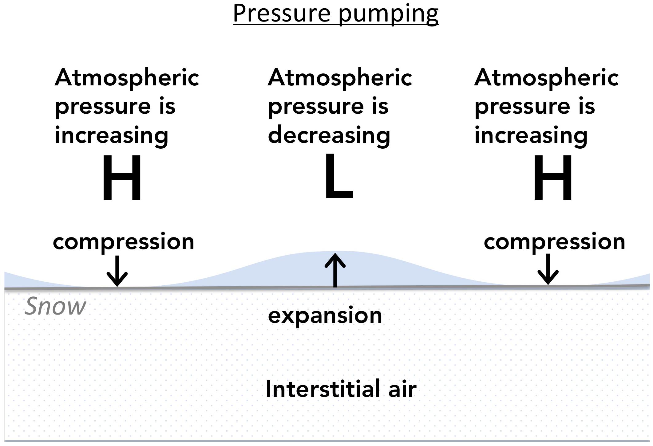
Figure 1. Increasing pressure compresses atmospheric air into the snowpack and decreasing pressure allows saturated air (denoted in blue) near the snow surface to translate into the atmosphere. Successive pulses of influx and efflux generate an upward flux of water vapor if the air above the snow is subsaturated. As shown, the horizontal axis is spatial but could rather be temporal.
Large amplitude pressure changes caused by synoptic weather patterns are too infrequent to significantly impact vapor flux by bulk air displacement. However, wind flow over surface rugosities and turbulence generate pressure changes at high enough frequencies to impact vapor exchange if their amplitude is sufficient. CB89 and Albert (2002) theorized that wind blowing over roughness elements stimulates local pressure gradients that cause alternating zones of preferential sublimation and deposition. The potential for turbulence to generate pressure changes with sufficient amplitude to enhance sublimation remains an open question. The basis for neglecting high-frequency (>0.1 Hz) pressure changes as a process that can enhance sublimation has relied on pressure measurements collected over an agricultural field (Elliot, 1972) rather than snow. Using Elliot’s (1972) results, CB89 developed an empirical formula to diagnose perturbation pressure as a function of wind speed:
where M is wind speed (m s–1) at 5 m height and p′ is the amplitude of a wind-induced pressure perturbation (Pa). In this paper, we investigate the potential for pressure pumping to enhance surface snow sublimation and thereby contribute to snow water equivalent (SWE) loss. Our methodology includes field experiments and empirical modeling. First, we test the validity of Eq. (1) with measured values obtained in field experiments. Next, we examine the attenuation of pressure fluctuations with depth in snow by spectral methods. We then apply two empirical models to test the hypothesis that atmospheric pressure changes enhance upward vapor exchange in the presence of wind and a vapor pressure deficit above the snow surface.
We deployed the field experiment at three sites: Santiam Pass, OR, United States (1468 m elevation), Dutchman Flat Sno-Park (sic), Oregon (1905 m elevation) and Storm Peak Lab, CO, United States (3220 m elevation) to obtain measurements across a range of snow regimes. The Santiam Pass site was a relatively flat 1/4 ha meadow in sparsely wooded terrain; the Dutchman Flat site was a 13 ha, open (nearly unvegetated) site; Storm Peak Lab was a high-altitude site with gently sloped terrain toward the windward direction during the field campaign. Proximity of trees at the Santiam Pass site, orography at the Storm Peak Lab site, and differences in microtopography between all three sites influenced turbulence intensity and perturbation pressure amplitude. Generally smooth snow cover was investigated in this experiment although we cannot preclude the possibility that topography and surface rugosities were consequential instigators of pressure fluctuations. The thrust of this experiment is to determine the role of pressure changes for vapor transport rather than quantifying the relative impact of different factors that generate these pressure changes. The highest winds in this experiment were recorded at Storm Peak Lab, however, these high winds were accompanied by blowing snow that invalidated sonic anemometer measurements and are thus not included in the presented results. Deployments are organized as cases in Table 1.
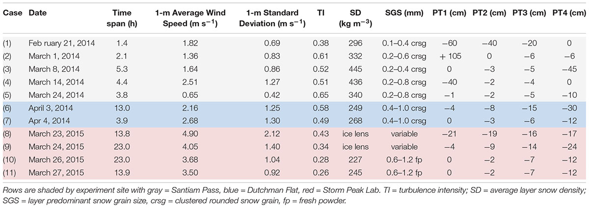
Table 1. Case numbers, associated dates and sensor heights relative to the snow surface for each deployment.
The experimental setup (see Figure 2) can be deployed within an hour, minimizing the likelihood that site conditions, such as surface snow characteristics, evolve during the data acquisition period. A Campbell Scientific Irgason (Logan, UT, United States) was mounted on a low-profile tower by means of a boom attached nominally 1 m above the snow surface. The Irgason transducer head was oriented into the prevailing wind 1.5 m upwind of the tower and leveled. 3-D wind speed and direction as well as CO2 and water vapor concentrations were logged at 20 Hz on a Campbell Scientific CR-3000 logger. This logger was time-synchronized with a second CR-3000 logger by means of a Campbell Scientific model GPS16X-HVS antenna and synchronizing software running on each logger. Precision in timing of the two loggers was approximately 10 μs according to the GPS antenna manual, well above the data acquisition frequency of 20 Hz.
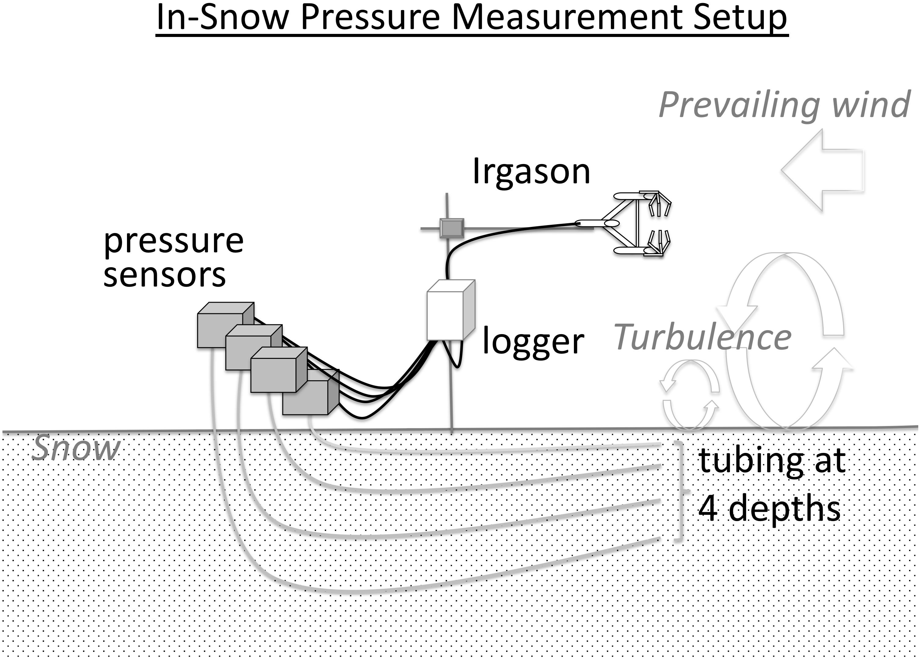
Figure 2. Schematic of the experimental setup. Pressure sensors measure at 4 depths in the snow through flexible tubing. A Campbell Scientific Irgason mounted ∼ 1 m above the snow measures 3D wind components at 20 Hz. Data are stored on a CR-3000 logger mounted on the low-profile tower.
The second CR-3000 logged pressure measurements from four Paroscientific Model 216B pressure sensors. These pressure sensors operated over a 300 hPa (800 hPa to 1100 hPa) range with 0.0001% resolution resulting in 0.03 Pa precision (Paroscientific Inc., 2013). In a previous pressure pumping study, Drake et al. (2016), referred to as D16, used Setra Model 264 relative pressure sensors for in-snow pressure measurements. Relative pressure sensors require a low-pass pressure sink to avoid pressure changes that exceed instrument capacity. By design, a pressure sink gradually leaks air so an increasing fraction of low-frequency energy was not captured as averaging timescale increased for the D16 study. In contrast, the absolute pressure sensors used in the present study did not require a pressure sink so low-pressure energy (the extent of which is defined by the time series length) is fully captured allowing pressure variance measurements over a broader range of frequencies. We note that high elevation site Storm Peak Lab exceeded the advertised lower bound for the Paroscientific pressure sensors used for this study. Paroscientific staff verified that the precision of our measurements was valid over the measured pressure range.
As will be described in the section “Model Calculations” we coded two empirical models in MATLAB to obtain order of magnitude estimates of pressure-enhanced sublimation rate based on pressure and wind measurements. The first model, named the simplified Monin-Obukhov (M-O) model, essentially counts water vapor molecules that have sufficient displacement to exceed the aerodynamic roughness length and become candidates for scouring by the atmosphere. An efficiency factor accounts for the stochastic nature of near-surface mixing. The second model, named the Gaussian model, approximates enhanced sublimation from statistical considerations (developed in the manuscript) and is also initialized by field-based measurements.
We formalize definitions for pressure “perturbations” and “fluctuations” as deviations from a defined mean and we refer to successive pressure changes as “excursions” in this paper. As such, “pressure perturbations” refer to a collection of individual pressure fluctuations and “perturbation pressure” is the time-integrated influence of these individual pressure changes. In panel (A) of Figure 3, pressure fluctuations correspond to wind speeds shown in panel (B). Pressure measurement depth was 12 cm in 227 kg-m–3 density snow (case 10). We minimized dynamic pressure effects due to wind blowing directly across the open end of the tubing by using subsurface pressure measurements for comparison with Eq. (1). Comparing panels (A) and (B) it is evident that higher wind speeds correlate with greater variability in pressure, consistent with D16. In panel (A), 20 Hz pressure fluctuations are relative to a 1-s block-averaged mean (orange) and 10 s fluctuations are relative to a 1-min block-averaged mean (blue). Here, we introduce a notation that describes the pressure data acquisition interval in superscript and the time averaging interval in subscript, both with units of seconds. For example, , refers to pressures acquired at 20 Hz (0.05 s interval) relative to a 1-s time average. Comparing , fluctuations (orange) with , fluctuations (blue) in Figure 3A, it is evident that lower frequencies tend to have greater amplitudes and longer timescales, consistent with findings in D16. This result is expected over the inertial subrange, the energy range for which larger scale eddies sustain smaller scale eddies and which contains the bulk of turbulent kinetic energy (Stull, 2012).
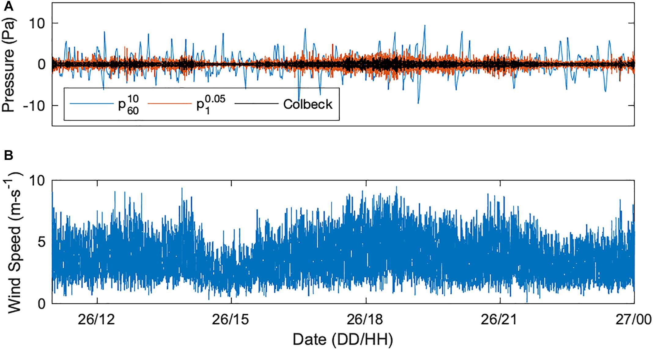
Figure 3. Panel (A) shows the in-snow (12 cm depth) pressure fluctuations to wind forcing at 1.2 m shown in the bottom panel (B) for March 26, 2017 at Storm Peak Lab (case 10). In panel (A), the blue line delineates 10 s perturbations from 1-min averages (), the orange line delineates 20 Hz perturbations from 1 s averages () and the black line delineates the theoretical prediction from Eq. 1.
The black line in panel (A) corresponds to values computed using Colbeck’s empirical formula Eq. (1) with wind speed logarithmically corrected from 1.2 to 5 m for a neutrally stable surface layer and assuming a 0.24 mm roughness length (from Gromke et al., 2011). Eq. (1) was developed using 10 Hz data above a rough surface (agricultural field) so the black line should exhibit greater amplitude than the 20 Hz (orange) line yet it is notably smaller. The difference between the Eq. (1) result and the result is further underscored by noting that the curve represents a subset of measured perturbation pressure whereas the Eq. (1) prediction represents the expected perturbation pressure integrated over a broader range of frequencies. For this case, Eq. (1) under-predicts the amplitude of surface perturbation pressure even though the pressure measurements are at 12 cm depth. This result was repeated for all cases and indicates that Eq. (1) mischaracterizes and underestimates the influence of perturbation pressure as a function of wind speed over snow. In the section “Materials and Methods,” CB89 does not indicate whether a pressure change is computed as a perturbation from a mean or as an excursion from the previous measurement. If they are excursions, then Eq. (1) underestimates pressure fluctuations by an even greater amount than shown in Figure 3, as will be discussed in the section “Spectral Dependence of Perturbation Pressure Attenuation.” It is also possible that Eq. (1) was developed from the standard deviation of pressure as a function of wind speed, in which case it still mischaracterizes observed measurements.
We summarize bin-averaged in-snow pressure perturbations vs. bin-averaged 20 Hz wind speed for cases 2 through 11 in Figure 4A. The timeseries for case 1 was too short to include in this analysis. Data are shown for the topmost (closest to snow surface) pressure measurement for the remaining cases (see Table 1). magnitude is much smaller than Figure 3 suggests because, for very short time scales, many perturbations are nearly zero whereas Figure 3 visually emphasizes large magnitude perturbations. The measure represents a small fraction of the total pressure perturbation field but it provides insight into the relationship between wind forcing and pressure response for different field deployments because the large number of measurements increases statistical significance. Comparing cases 6 and 7, and cases 10 and 11 in Figure 4A, we find that, for given snow properties and site, the in-snow pressure response to wind forcing is repeatable. Correspondence of cases 2 and 5 show that at low wind speed snow properties regulate perturbation pressure response. Increased perturbation pressure at a given wind speed for cases 8 and 9 indicate that ice lenses do not inhibit pressure perturbation at shallow depth but may actually enhance them by constraining the airspace available to relieve a given pressure gradient.
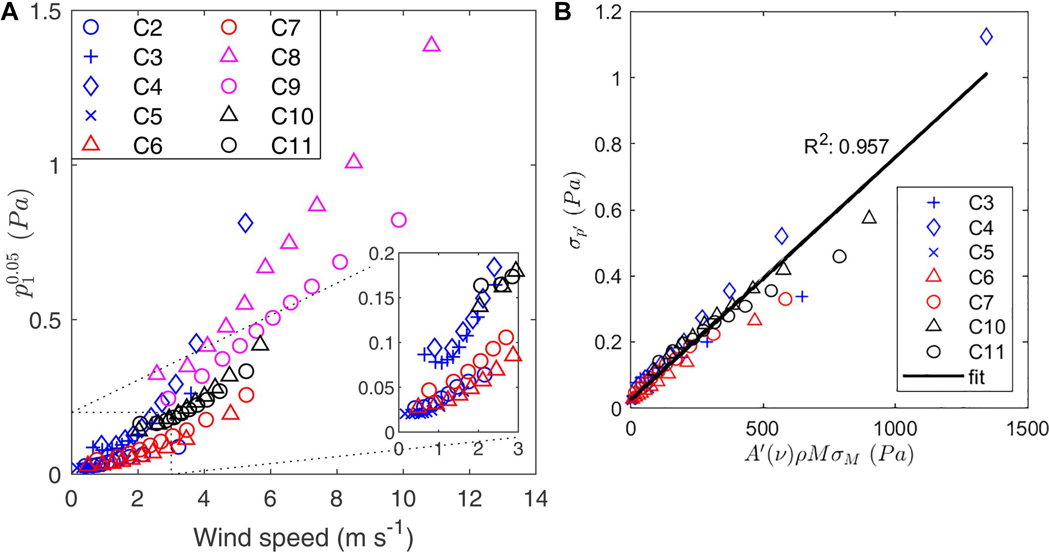
Figure 4. Ranges for pressure fluctuation vs. bin-averaged wind speed for deployments color-coded by site with an inset for wind speeds below 3 m-s– 1 (panel A). Panel (B) shows a similarity relationship between the standard deviation of perturbation pressure with the product of snow density, wind speed and the standard deviation of wind speed.
Rather than performing a curve fit between wind forcing and perturbation pressure response for each case we seek a similarity relationship that produces a generalized curve fit that is valid across cases. Based on Buckingham Pi dimensional analysis (Bertrand, 1878), we find one possible similarity relationship that relates wind speed, a length scale (such as depth, D), and the specific surface area of snow (SSAM that forms a dimensionally correct relationship:
Where is the standard deviation of perturbation pressure at a given frequency, σMis the standard deviation of wind speed, ρ is snow density, M is wind speed, and A(v) and A′(v) are frequency-dependent functions that are not yet determined. We experimented with permutations of (dimensionally equivalent) M and σM and found the correlation between the product of wind speed and the standard deviation of wind speed with the standard deviation of perturbation pressure was optimized compared with either M2 or . We hypothesize that the correlation between perturbation pressure and the product of M and σM is greater than the correlation between perturbation pressure and either M2 or because the perturbation pressure field is influenced by both near and far-field wind velocity changes. The standard deviation of wind speed better expresses near-field perturbation pressure generation and M expresses both near and farther field perturbation pressure generation. This hypothesis is consistent with findings by Monin and Yaglom (1975) as quoted by Albertson et al. (1998):
“it is possible that comparatively far regions of the flow make non-negligible contributions to the pressure fluctuations at a point.”
Eq. (2) is supported on physical grounds by the Bernoulli equation, which relates pressure changes to the square of the fluid velocity and theoretically by Eq. (15) in Katul et al. (1996), which relates σp’ to the square of friction velocity. There may be other relevant variables that we have not identified in Eq. (2). If so, the influence of these variables is incorporated into A′(v). Since Eq. (2) is derived from dimensional analysis we denote an approximate equivalence between the lhs and rhs rather than equality. Lacking direct measures of SSAM we note that snow density is proportional to a negative power of SSAM (Matzl and Schneebeli, 2006; Domine et al., 2007) although with significant variability. Substituting the inverse of the snow density into Eq. (2) preserves the influence of SSAM on perturbation pressure response and dimensional integrity. Figure 4B shows the result of this approximation to Eq. (2), excluding cases with ice lenses (8 and 9) as well as case 2. For case 2 we noted an anomalous increase in σM as wind speed increased, which we attribute to the close proximity of the pressure sensor shield (that was present only for case 2 relative to the sonic anemometer. The coefficient of determination between the remaining cases was 0.957. As shown by the smooth curve for case 2 in Figure 4A, the presence of the pressure shield did not unduly influence measured wind speed. We computed A′(v) from the slope of Figure 4B by block averaging 20 Hz data over incrementally larger blocks so that we could use A′(v) to estimate in the section “Discussion of Field Observations” of this manuscript. The magnitude of A′(v) was 0.0006 at 2 Hz (10 data points acquired at 20 Hz) and increased with decreasing frequency, plateauing at 0.029 Hz with a value of 0.0015. Below 0.029 Hz, can be estimated from a 4th order polynomial with coefficients (−0.03, 0.06, −0.021, 0.053, 1.4) × 10–3.
We next employ spectral analysis to investigate how pressure perturbation energy varies with pressure change frequency. For each case we performed spectral analysis for each pressure sensor to gauge spectral attenuation of pressure gradients. When performing spectral analysis, missing data were gap-filled with data randomly chosen from nearby points in the time series (Falge et al., 2001). Missing data comprised no more than 0.02% of the data record so our results should be insensitive to the choice of gap-filling algorithm. Inspecting the resultant spectra and noting that it did not unduly introduce artifacts such as spectral ringing verified this gap-filling method for missing data.
Figure 5A shows the pressure spectra for case 2. These spectra were generated by averaging 2048-point FFTs of de-trended 20 Hz pressure data resulting in a spectral bandwidth of 1.7 (∼2) min. We applied a Hann window to reduce spectral leakage (Chelton, 2015). As expected, there was greater pressure variance at all frequencies 1 m above the snow (blue line) than at 6 cm depth (green and gold lines) in Figure 5A. Two independent measurements at 6 cm depth suggest reproducibility in spectral attenuation at frequencies below 4 Hz. Consistent with Elliot (1972), pressure spectra logarithmically decreased with increasing frequency so the magnitude of the integrated pressure variance is dominated by low frequencies.
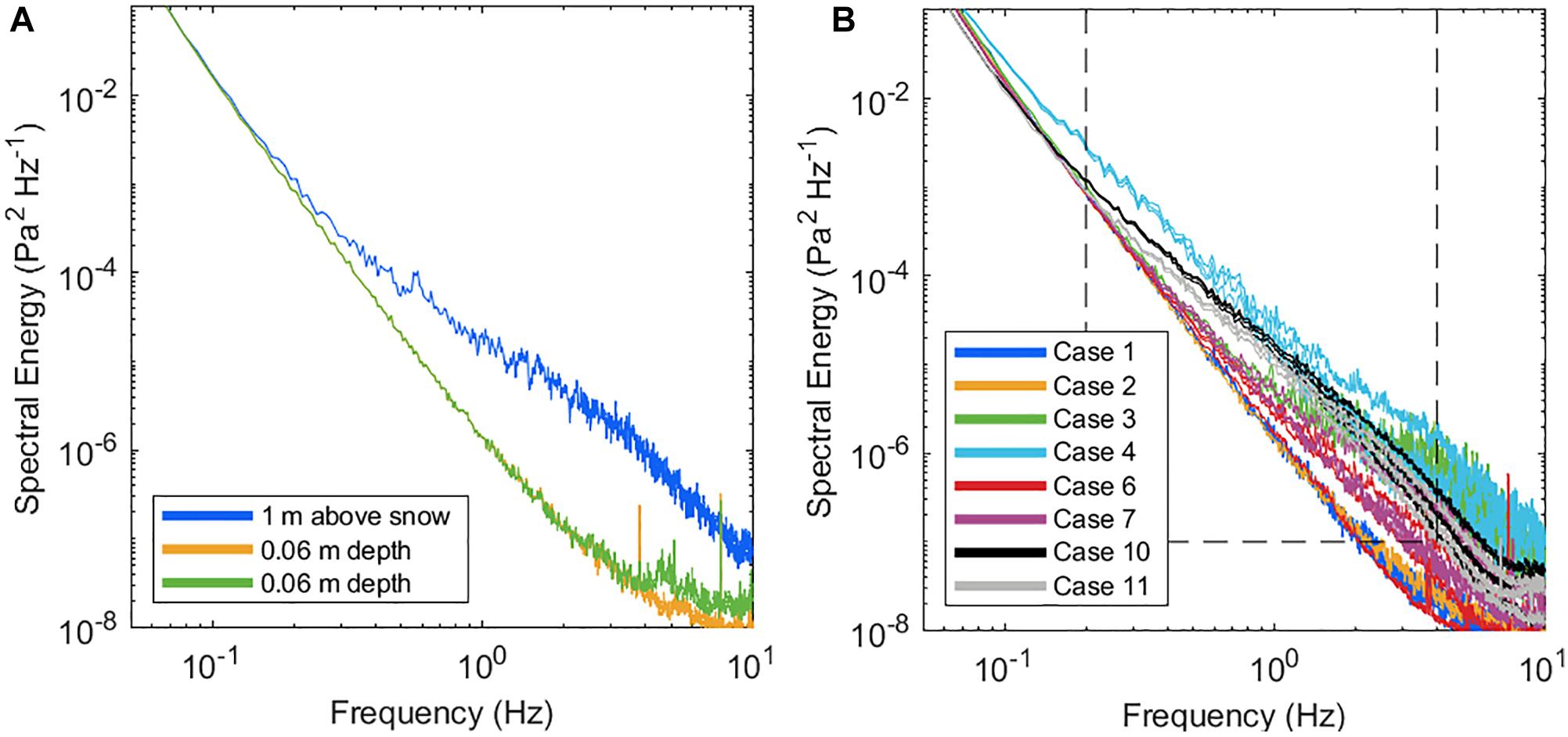
Figure 5. Pressure spectra at 1 m above the snow (blue) and 6 cm below the snow surface (green and gold) for case 2 (panel A), and at each depth for representative cases (panel B, see Table 1). Duplicate measurement depths in panel (A) delineate perturbation pressure reproducibility at frequencies below 4 Hz. The dashed line in panel (B) delineates the extent of frequencies and spectral energy that were used to analyze spectral power attenuation. For a homogenous layer, spectral energy measurements at a given depth (6 cm for case 2) are repeatable (panel A).
For the range of snow densities (227–445 kg m–3) and regardless of surface snow topographical differences between cases, relative pressure attenuation below 0.2 Hz was insignificant (Figure 5B). This ∼0.2 Hz transition frequency compares closely with the 0.1 Hz result based on numerical simulations in Albert (1993) and measurements in D16. These results do not necessarily mean that high frequency pressure changes are inconsequential because it is possible that pressure changes with frequency > 0.2 Hz generate sufficient vertical displacement to enhance vapor exchange with the atmosphere, even with attenuation. Therefore, we next determine the attenuation of perturbation pressure with depth in snow.
D16 found a decay of high-frequency spectral energy with depth, consistent with the observations presented here. We ascribe the difference in spectral attenuation with depth between D16 and this study to differences in snow layers in D16 that we largely avoided by design in this experiment. Consistent decay of high-frequency pressure perturbations with depth in an approximately homogenous snow layer enabled computation of spectral attenuation of pressure variance with depth. Acoustic attenuation at frequencies below 200 Hz is small and decreases with decreasing frequency (Maysenhölder et al., 2012). Nevertheless, we employ an equation that describes acoustic attenuation as a power law (Szabo, 1994):
where v is perturbation pressure frequency, p′(v) is perturbation pressure amplitude at a given snow depth (Δz), is perturbation pressure amplitude at the snow surface and α(v) is the attenuation coefficient. Eq. (2) states that attenuation of pressure waves in snow increases with pressure perturbation frequency and/or depth in snow.
To estimate the spectral attenuation of pressure fluctuations with depth in snow we subset the pressure spectra in Figure 5B to the data delineated by the dashed lines. Pressure spectra with power less than 10–7 Pa2-Hz–1 flatten out at the noise floor of the pressure sensors. At frequencies greater than ∼0.4 Hz aliasing and poor reproducibility manifest (as shown in Figure 5A) so we pruned these data from subsequent analysis. We analyzed cases that had a pressure measurement at the snow surface to provide a consistent baseline. For each pressure sensor we calculated the spectral slope by bin-averaging perturbation pressure in frequency space so that each frequency bin contributed equivalently to the linear correlation (Figure 6A). We then plotted spectral slope as a function of depth in snow in Figure 6B. The linear regression in Figure 6B is the average change in spectral slope with depth for analyzed cases. Spectra for case 8 were not sufficiently linear and were thus excluded from spectral slope comparison.
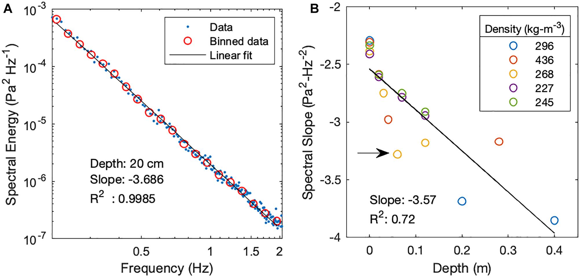
Figure 6. Computation of spectral slope for the 20 cm depth pressure sensor for Case 1 (panel A). The change in spectral slope with depth can be precisely computed only with cases for which spectral slope have R2 values greater than 0.9. For each snow layer we compute the spectral slope relative to the sensor at the snow surface (panel B). Results show a linear increase in the absolute value of spectral slope with depth. The average spectral slope is –2.54 to –3.57d for depth (d) in the snow. The arrow in panel (B) points to an anomalous data point that has a larger absolute magnitude of slope than the data point below it.
For cases with a surface pressure measurement, we found an average spectral slope (S as a function of depth in snow:
where Δz is measurement depth in snow in meters. The correlation coefficient was 0.72 and included one data point (see arrow in Figure 6B) that had greater absolute magnitude in spectral slope than the measurement below it. We note the best correlations were found for the two lowest density cases (227 kg-m–3 and 245 kg-m–3) and attribute this strong correlation to homogeneity in snow matrix characteristics through the snow layer. Eq. (4) is an empirical expression for estimating spectral attenuation of pressure perturbations in seasonal snow as a function of depth and could be employed in a model with appropriate consideration of the limits and assumptions that were used to derive it. The average spectral slope of surface pressure measurements was −2.35 ± 0.05, which is smaller in magnitude than the calculated value of −2.54 based on the linear correlation. So, there is a slight bias in the slope in Eq. (4) due to a step change in spectral slope at the snow interface. This step change in spectral slope was noted for snow layers in D16 and we similarly interpret this spectral slope step change at the snow surface as an impedance signature.
The empirical formula in Eq. (4) describes the slope of pressure variance due to frequency-dependent attenuation with depth in snow. We integrate Eq. (4) to derive an equation for spectral power as a function of depth in snow:
where P(v) is spectral power at a given frequency and p0 is a reference spectral power. For example, referring to Figures 5B, 6B and using Eq. (5) the spectral power at 2 Hz is:
where we have used 10−3Pa2Hz−1 as the spectral power at the 0.2 Hz reference frequency. At 1 cm depth the power at 2 Hz is 8% smaller. In the section “Model Calculations” we will use Eq. (5) to estimate the attenuation of perturbation pressure at each frequency with depth in snow.
Massman et al. (1997) attributed high frequency attenuation to spatial averaging over the extent of the hose they used to acquire pressure measurements. We observe a similar high frequency attenuation although our measurement apparatus has very small (7.5 mm) extent. D16 noted that high-frequency attenuation of pressure variance is greater than predicted by 1-dimensional models, a result that is consistent with the Clarke and Waddington (1991) (hereafter referenced as CW91) hypothesis that high-frequency pressure energy is distributed amongst three dimensions rather than fully attenuated in a single dimension. Spherical divergence therefore accounts for the bulk of apparent attenuation with depth. This hypothesis is consistent with the physical constraints that large-scale pressure changes are more hydrostatic (planar) and small-scale pressure changes are more isotropic (spherical). Additionally, the relative magnitude of the return to isotropy term in the TKE budget equation increases as the spatial scale decreases (Stull, 2012).
Our experimental results as well as those presented in CW91 and D16 show that a power law function describes attenuation of pressure perturbations with frequency and depth. We therefore reconsider the discrepancy between these experimental results and the theoretical prediction of exponential decay that was addressed in CW91. The authors attributed this discrepancy to either localized pressure disturbance caused by the measurement setup or an over-reliance on Taylor’s Hypothesis. We conclude it is unlikely that a given measurement setup would produce this systematic difference for different snow permeability and over a range of depths spanning up to 60 cm. If, as CW91 suggest, the experimental apparatus artificially produces spectral attenuation that follows power law behavior rather than exponential decay, then we would expect high-frequency attenuation would approach exponential decay with increasing depth and snow density, where disturbance due to the experimental apparatus declines. Our experimental results do not show this tendency. Neither do the results in D16 using a different experimental design and different pressure sensors. This lack of a systematic change in power law behavior with changes in snow depth and density also rules out the theory that an over-reliance on Taylor’s hypothesis has skewed the experimental results. We suggest a third alternative: that the fundamental assumption of the equation that describes the attenuation of pressure perturbations (CW91, Eq. 1) should be modified such that it has a solution that describes attenuation as a power law rather than exponential decay with frequency and depth.
Since Eq. (1) underestimates perturbation pressure and also fails to describe the distribution of pressure fluctuations, we seek an alternative formulation that reproduces the observation that perturbation distribution broadens both with increasing wind speed and averaging time scale. The tails of this distribution would then capture the influence of infrequent, large amplitude pressure fluctuations. We model the range of perturbation pressure as a Gaussian distribution (Borisov et al., 2007) recognizing that a Gaussian velocity profile can produce a Gaussian pressure fluctuation profile with exponential tails (Holzer and Siggia, 1993):
for which the peak width is a function of averaging time scale and wind speed. A Gaussian distribution may not be representative for a turbulent regime (Borisov et al., 2007) and perturbation pressure distributions in this study exhibited a truncated Gaussian shape that was most pronounced for short time averaging intervals (not shown). However, we assume a normal distribution as a starting point with the noted qualifications. With Eq. (2), one can use wind speed to estimate the standard deviation of pressure perturbations as a function of wind forcing. Assuming a normal distribution, the Bienaymé-Chebyshev inequality provides an estimate for the fraction of pressure perturbations that exceed a given value based on the standard deviation of the data set:
where k is the number of standard deviations from the mean. For example, the maximum fraction of values greater than 10 standard deviations from the mean is ≤0.01. With Eq. (8) one can estimate an upper limit for the fraction of pressure perturbations that exceed a critical value. We reserve further discussion of this Gaussian model for an application of it in the section “Model Calculations”. An advantage of using a statistical model rather than an equation having the form of Eq. (1) is that it computes a distribution of perturbation pressure, which is more realistic than a mono-valued relationship between wind forcing and perturbation pressure response.
A realistic approximation for sublimation rate enhancement accounts for the atmospheric capture efficiency based on frequency and vapor pressure deficit. We propose the following relationship to describe the integrated sublimation rate enhancement as a function of surface area, vapor pressure deficit and vapor capture efficiency:
where S is the integrated enhancement to sublimation rate for all relevant frequencies, ϕNis snow porosity, ∈(v,m) is the efficiency by which water vapor is captured by the wind at speed M for pressure changes at frequency v, and Sv is the maximum theoretical sublimation rate for that frequency. The quantity (qs−q) is the normalized vapor pressure deficit and equals zero when air above the snow is saturated.
In Monin-Obukhov (M-O) boundary layer theory, displacement length is the height above the surface at which a logarithmic wind profile initiates. Typical applications of displacement length are for winds above uniform agricultural crops and dense forests. Clifton et al. (2008) found evidence of in-snow ventilation due to wind and hypothesized a negative displacement length. M-O theory utilizes the notion of an aerodynamic roughness length (z0), which is defined as the height above the surface where wind speed is zero. We apply M-O boundary layer theory to approximate the convolution of frequency and amplitude and consider middle frequencies for which it may be possible that pressure perturbations have sufficient magnitude and frequency to enhance sublimation.
Now that we have an estimate for the distribution, magnitude and attenuation of pressure perturbations as a function of frequency we can attempt to model the wind pumping process. To facilitate comparison between cases we assume a constant vapor pressure deficit of 1% for all cases, which is representative of air very near the snow surface. We approximate the exchange efficiency in Eq. (9), ∈(v,m), as an exponential decay function below z0. The actual values of ∈(v,m) are not known. For the model simulations we used an equation of the form:
where we arbitrarily assume coefficients α = 10−6 and β = 1. Unknown coefficients α and β constrain our ability to assign absolute sublimation rates to model results and is a potential topic for future study. This approximation formalizes the M-O assumption that water vapor molecules must traverse the roughness layer to be candidates for capture by the atmosphere. The aerodynamic roughness length stochastically describes the mixing influence of ephemeral turbulent eddies rather than describing the height of a “lid” of air above the snow. For model simulations, we utilize an aerodynamic roughness length of 0.24 mm for fresh snow from Gromke et al. (2011).
We implemented a surface exchange model to test the functional relationship between perturbation pressure frequency and vapor exchange rate. In this model, vapor exchange caused by turbulent eddies is approximated by hydrostatic pressure changes relative to the aerodynamic roughness length. At each frequency we computed pressure deviations between successive measurements. If the hydrostatic height change exceeded the aerodynamic roughness length then we computed the displacement length above z0. We then computed water vapor flux as a function of the vapor pressure deficit and perturbation pressure frequency. Before summing the flux for each frequency we applied the frequency-dependent efficiency factor described in Eq. (10). We note that the efficiency factor adjusted the magnitude of the vapor exchange rate but the coefficients were tuned such that they did not change the functional shape or the frequency of maximum vapor exchange of the resultant curve.
We also implemented an empirical model utilizing Eqs. (2, 7, and 8) to obtain a distribution of pressure perturbations as a function of wind forcing and snow density. For a given wind speed and for each perturbation pressure frequency we use Eq. 2 to compute σp. As with the simplified M-O model we determine the high frequency attenuation (Eq. 5) for subsurface pressure sensors. We then use the Bienaymé-Chebyshev inequality (Eq. 8) to determine the subset of water molecules that could have sufficient amplitude to generate a hydrostatic adjustment equal to or greater than z0, assuming a normal distribution. We then subdivide pressure perturbations into many narrow ranges of time scale averages and integrate the vapor exchange rate for each frequency and apply the efficiency factor, ∈(v,m) (Eq. 10). In summary, this Gaussian model requires as input the wind speed, snow density, aerodynamic roughness length, vapor pressure deficit and an estimate of the efficiency factor to generate an estimation of surface snow sublimation rate. Clearly, many other state variables are important including snow grain characteristics, temperature, stability, turbulence intensity, etc. To some degree, the influence of these factors are represented in the A′(v) term in Eq. 2, however, the relative importance of these factors are not yet known.
We plotted pressure-induced sublimation rate as a function of pressure change period in Figure 7A for cases 2, 7, and 10. The average wind speed for these three cases span a representative range of average wind speed for all cases. At 20 Hz, displacement length for these cases was insufficient to exceed the aerodynamic roughness length and vapor exchange was negligible. For cases 2 and 7 sublimation enhancement was vanishingly small at all frequencies. For case 10, pressure fluctuations generated vertical displacements that exceeded the aerodynamic roughness length with sufficient frequency to enhance sublimation. As the time-averaging interval increased, pressure fluctuation amplitude increased and the vapor exchange rate increased to a maximum at ∼0.5 s period length for case 10. At longer periods the vapor exchange rate decreased with increasing oscillation period as the influence of decreasing frequency prevailed over the increasing amplitude of pressure fluctuations. Sensitivity analysis of case 10 using vapor pressure deficits of 0.1, 0.5, and 2% yielded a linear change in calculated sublimation rate of 10, 50, and 200%, respectively, compared with the benchmark value (1% VPD).
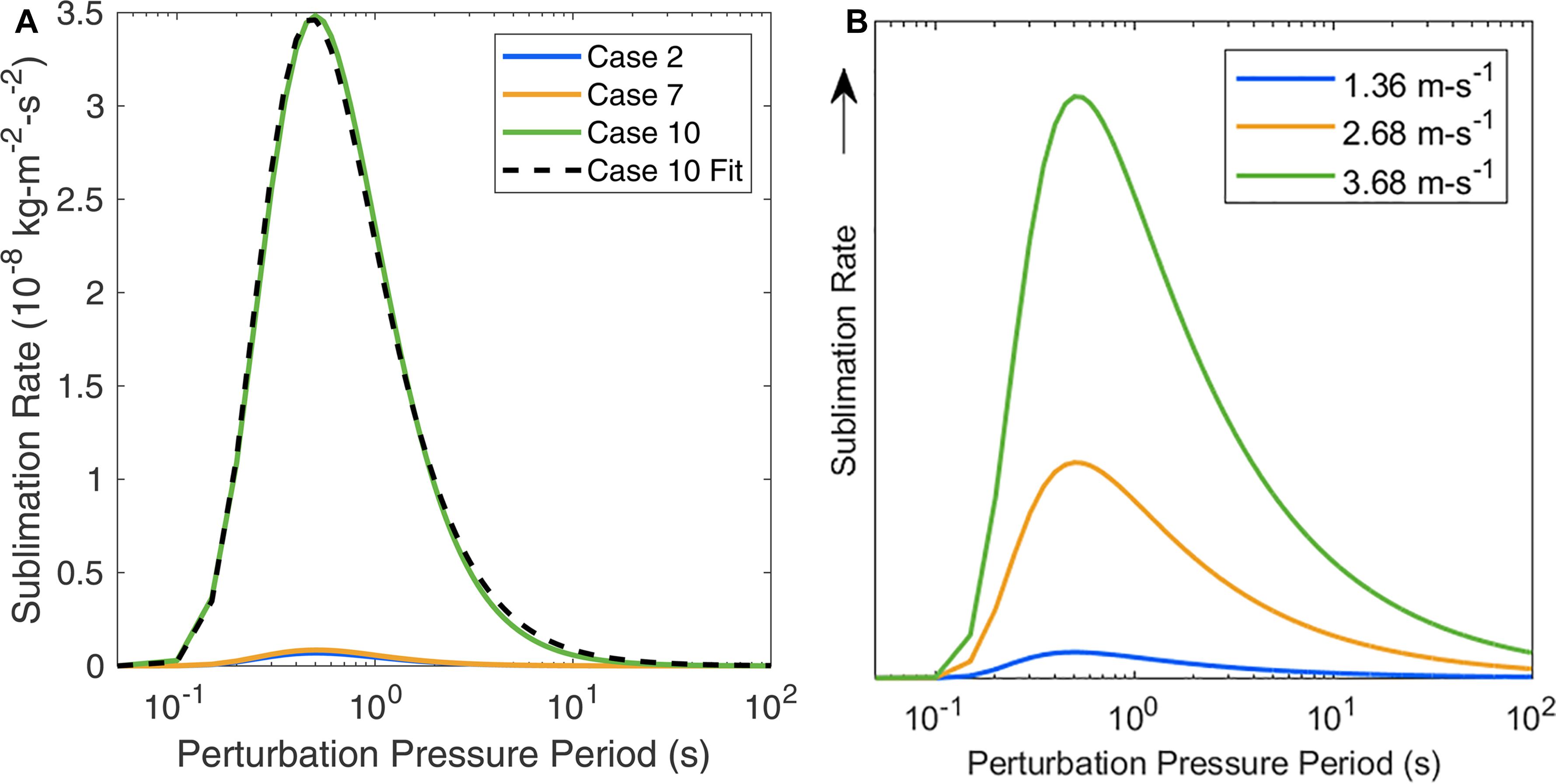
Figure 7. Simplified M-O model results in panel (A) show sublimation rates as a function of oscillation period for cases 2, 7 and 10. The integral of the curve is the sublimation rate for each case. Initializing the Gaussian model (panel B) with the average wind speeds for cases in panel (A), we find a similar functional relationship between the simplified M-O and the Gaussian model. The Gaussian model overpredicts the sublimation contribution of longer period pressure fluctuations and also overpredicts sublimation at low wind speed for these cases.
We initialized the Gaussian model using the same average wind speed for cases shown in Figure 7A and plotted the results in Figure 7B. Comparing Figures 7A,B we find that the simplified M-O model and Gaussian model produce a similar functional form. The Gaussian model produced higher sublimation rate in the tail of the distribution and also larger sublimation rates at lower wind speeds than the simplified M-O model. This discrepancy suggests a need to tune the Gaussian model to accommodate pressure distributions that are not sufficiently normal, for example, by employing a truncated Gaussian functional form. When applied more broadly to data that were not part of this study, it is possible that complexity in surface processes would preclude the existence of a single distribution that would accurately relate pressure fluctuation amplitude and sublimation rate. However, for this set of cases the correspondence of the functional relationship between the Gaussian model and the simplified M-O model indicates that the influence of high frequency pressure perturbations can be modeled using a power law relationship that approximates σp from wind speed. For these case studies, the computed vapor flux enhancement was strongest for periods ranging from 0.2 s to 10 s. Both the simplified M-O model and the Gaussian model indicate that higher amplitude turbulence and/or smaller aerodynamic roughness length pushes the range of maximum vapor flux toward shorter periods.
We now estimate the magnitude of enhanced vapor exchange by pressure pumping from a sublimation rate equation adapted from Albert and McGilvary (1992):
where hM is the mass exchange coefficient, as is the surface area of the ice matrix per volume of snow, pSAT is saturation vapor density, pv is vapor density and δz is the active layer depth. This equation applies to a well-ventilated snow sample. A natural snow surface is not as efficiently ventilated, which is one reason that we introduced the efficiency parameter in Eq. (9). Using intermediate values for the specific surface area per unit mass and snow density for powder snow from Table 1 in Domine et al. (2007) we find:
In this example we utilize improved values for hM from Neumann et al. (2008). For a 5 mm active snow depth (estimated from Clifton et al., 2008), hM = 5×10⁻³ms−1, pSAT = 5×10⁻³kgm−3 and pv = 0.99pSAT the sublimation rate from Eq. (11) is 8.9×10⁻⁶kgm−2s−1. Substituting pSNOW = 340kgm−3 and SSAM = 20.6m−1kg−1 from the same table for snow having rounded grains results in a sublimation rate of 8.8×10⁻⁶kgm−2s−1, similar to powder snow. We anticipate that the active depth for dense snow is less than powder snow so the sublimation rate of dense snow would be correspondingly reduced. These estimates are highly sensitive to vapor pressure deficit but is of the order of seasonal sublimation rates derived from field experiments by Reba et al. (2012)4.5×10⁻⁶kgm−2s−1and Molotch et al. (2007), 4.7×10⁻⁶kgm−2s−1. This scale analysis likely overestimates enhanced sublimation rate because the active snow depth is not evenly ventilated as in Neumann et al. (2008). Nevertheless, scale analysis shows that the magnitude of sublimation enhancement is too large to dismiss wind-induced pressure perturbations as a consequential process for sublimation enhancement and prompts further investigation.
In light of these results, we reexamine Stössel et al. (2010), referenced hereafter as S10, in which the authors assessed deposition and sublimation rates of surface hoar at an alpine site. They found that eddy flux calculations underestimated deposition rates and underestimated sublimation rates of surface hoar compared with snow lysimeter measurements (see S10, Figure 8). If we assume the snow lysimeter measurements in S10 accurately represent sublimation and deposition rates, then we can interpret their results in the context of how pressure changes influence vapor flux. For the S10 site, deposition was favored during nocturnal, weak wind episodes. In these conditions, wind-generated pressure changes would be weak and have vanishingly little influence on deposition rate. Eddy flux underestimation of deposition rate in these conditions relative to the snow lysimeter could be rather caused by longwave cooling of the snow surface, which would accelerate deposition rate in a supersaturated environment. If the eddy flux measurements accurately depict net downward transport of water vapor, then some of the water vapor that is depositing as surface hoar would need to come from the layer of air below the height of the eddy flux measurements (including interstitial pore space). Crystal growth would be maximized at the snow surface where the combination of longwave cooling and vapor supply are maximized and at sites where microphysical processes favor deposition (as noted in S10). Since windpumping is minimal, interstitial vapor transport would be diffusive. For windy conditions it is possible that eddy flux measurements are not capturing the effect of sublimation enhancement by pressure changes. As noted by the S10 authors, site complexity violates assumptions embeded in eddy covariance calculations so we cannot with confidence attribute the difference between snow lysimeter and eddy flux measurements to wind pumping. For both the S10 lysimeter receptacle and the natural snow surface, interstitial vapor flux would replace vapor lost at the snow surface, decreasing the vapor pressure deficit at the snow/atmosphere interface and increasing snow crystal longevity at the surface as observed by Hachikubo and Akitaya (1998). Clearly, analysis of the S10 results would benefit from a more complete theory of surface exchange processes.
The integral of the curve in Figures 7A,B is the sublimation rate over all perturbation pressure frequencies and the derivative of this function is the peak sublimation rate. We calibrated Figure 7A by integrating the curve for case 10 and linearly adjusting a function until the integral equaled a 5×10⁻⁶kgm−2s−1 sublimation rate (estimate above) to derive an order of magnitude estimate of peak sublimation rate. Using the MATLAB fittype() and fit() functions we found the fitted curve in Figure 7A as:
where τ is time period in seconds. For case 10, we plotted Eq. (13) as a black dashed line in Figure 7A over the range [0.05s, 1000s] using coefficients: a = −1.43×10⁻⁸±5×10⁻⁸, b = 0.0808 ± 0.002 and c = 1.159 ± 0.001. The curve fit matches the data well at frequencies relevant for sublimation enhancement.
Taking the derivative of Eq. (13) and setting it equal to zero yields the peak frequency:
which we solved numerically and found the peak sublimation rate at 0.48 s, which is the same as the empirical result (with peak period of 0.5 s).
Negative feedbacks reduce the rate of vapor exchange by wind pumping and lessen SWE reduction. For example, as winds increase snow grains saltate, become suspended and thereby saturate near surface air, diminishing the vapor pressure gradient needed for wind-pumping driven vapor exchange. Sublimation rounds snow crystals and glazes the snow surface by subsequent deposition. In contrast, saturation vapor pressure is an exponential function of temperature so warmer snow increases vapor exchange by pressure fluctuations relative to colder snow that otherwise has similar microphysical characteristics. A full reckoning of all vapor exchange process are needed to compare the relative roles of these processes and the interplay between them in various environmental conditions.
We find that the Colbeck (1989) equation defined in Eq. (1) underestimates and mischaracterizes the amplitude of wind-induced pressure perturbations that drive wind pumping. The standard deviation of wind speed is a useful statistical descriptor of wind pumping. However, when used to determine a threshold for air displacement it masks the influence of the less frequent, high-amplitude pressure perturbations that drive wind pumping. Spectral analysis of perturbation pressure suggested an empirical formula for estimating frequency-dependent attenuation of perturbation pressure with depth in snow. Perturbation pressure attenuation down to 60 cm depth was limited to frequencies above 0.2 Hz in close agreement with a theoretical treatment by Albert (1993). Combining our field measurements and model calculations with results from previous studies we estimate that water vapor flux enhancement by pressure pumping is maximized for pressure changes having period between 0.2 and 10 s and could be approximated by an expression of the form in Eq. (13). The magnitude of the enhancement of water vapor flux is poorly constrained because the exchange efficiency as a function of pressure perturbation frequency and other environmental factors is not known. An improvement in understanding how the perturbation pressure distribution changes with frequency and environmental factors would facilitate more accurate estimates of pressure-induced sublimation.
Over short timescales, turbulence combined with dry surface air is needed to generate noteworthy vapor exchange enhancement. In windy conditions, this pressure pumping process is persistent and pervasive so it may have a significant mass balance impact over seasonal time scales. In a natural environment it is difficult to discriminate pressure-induced sublimation enhancement from sublimation that is not spurred by pressure fluctuations. However, it is important to improve our understanding of the different processes by which snow sublimates if we aim to improve our ability in predicting the seasonal evolution of the snowpack.
SD authored the initial manuscript. CH and JS provided insights and edited it.
This publication was funded by the startup funding from the University of Nevada, Reno.
The authors declare that the research was conducted in the absence of any commercial or financial relationships that could be construed as a potential conflict of interest.
Thanks to Dr. Noah Molotch and Dr. Michael Durand for their support during the Colorado campaign, Lisa Dilley (USFS) for coordinating access to Dutchman Flat Sno-Park (sic), Dr. Ziru Liu and Rebecca Hochreutener for deploying equipment, and the three reviewers and the editor for their comments and suggestions.
Albert, M. R. (1993). Some numerical experiments on firn ventilation with heat transfer. Ann. Glaciol. 18, 161–165. doi: 10.3189/S0260305500011435
Albert, M. R. (2002). Effects of snow and firn ventilation on sublimation rates. Ann. Glaciol. 35, 52–56. doi: 10.3189/172756402781817194
Albert, M. R., and McGilvary, W. R. (1992). Thermal effects due to air flow and vapor transport in dry snow. J. Glaciol. 38, 273–281. doi: 10.3189/S0022143000003683
Albertson, J. D., Katul, G. G., Parlange, M. B., and Eichinger, W. E. (1998). Spectral scaling of static pressure fluctuations in the atmospheric surface layer: the interaction between large and small scales. Phys. Fluids 10, 1725–1732. doi: 10.1063/1.869689
Ayala, A., Pellicciotti, F., Peleg, N., and Burlando, P. (2017). Melt and surface sublimation across a glacier in a dry environment: distributed energy-balance modelling of Juncal Norte Glacier, Chile. J. Glaciol. 63, 803–822. doi: 10.1017/jog.2017.46
Bartlett, S. J., and Lehning, M. (2011). A theoretical assessment of heat transfer by ventilation in homogeneous snowpacks. Water Resour. Res. 47:W04503. doi: 10.1029/2010WR010008
Borisov, A. V., Kozlov, V. V., Mamaev, I. S., and Sokolovskiy, M. A. (eds) (2007). IUTAM Symposium on Hamiltonian Dynamics, Vortex Structures. Turbulence: Proceedings of the IUTAM Symposium Held in Moscow, 25-30 August, 2006, Vol. 6. Berlin: Springer Science & Business Media.
Bowling, D. R., and Massman, W. J. (2011). Persistent wind-induced enhancement of diffusive CO2 transport in a mountain forest snowpack. J. Geophys. Res. Biogeo. 116:G04006. doi: 10.1029/2011JG001722
Clarke, G. K. C., Fisher, D. A., and Waddington, E. D. (1987). “Wind pumping: a potentially significant heat source in ice sheets,” in Proceedings of the International Association of Hydrological Sciences Publication and the Physical Shape of Ice Sheet Modelling, Vancouver, 169–180.
Clarke, G. K. C., and Waddington, E. D. (1991). A three-dimensional theory of wind pumping. J. Glaciol. 37, 89–96. doi: 10.3189/S0022143000042830
Clifton, A., Manes, C., Ruedi, J. D., Guala, M., and Lehning, M. (2008). On shear-driven ventilation of snow. Bound. Lay. Meteorol. 126, 249–261. doi: 10.1007/s10546-007-9235-0
Colbeck, S. C. (1989). Air movement in snow due to windpumping. J. Glaciol. 35, 209–213. doi: 10.3189/S0022143000004524
Cunningham, J., and Waddington, E. D. (1993). Air flow and dry deposition of non-sea salt sulfate in polar firn: paleoclimatic implications. Atmos Environ. Part A Gen. Top. 27, 2943–2956. doi: 10.1016/0960-1686(93)90327-U
Déry, S. J., and Yau, M. K. (2002). Large-scale mass balance effects of blowing snow and surface sublimation. J. Geophys. Res. Atmos. 107:4679. doi: 10.1029/2001JD001251
Domine, F., Taillandier, A. S., and Simpson, W. R. (2007). A parameterization of the specific surface area of seasonal snow for field use and for models of snowpack evolution. J. Geophys. Res. Earth Surface 112:F02031. doi: 10.1029/2006JF000512
Drake, S. A., Huwald, H., Parlange, M. B., Selker, J. S., Nolin, A. W., and Higgins, C. W. (2016). Attenuation of wind-induced pressure perturbations in alpine snow. J. Glaciol. 62, 674–683. doi: 10.1017/jog.2016.53
Elder, K., Dozier, J., and Michaelsen, J. (1991). Snow accumulation and distribution in an Alpine Watershed. Water Resour. Res. 27, 1541–1552. doi: 10.1029/91WR00506
Elliot, J. A. (1972). Microscale pressure fluctuations measured within the lower atmospheric boundary layer. J. Fluid Mech. 53, 351–383.
Falge, E., Baldocchi, D., Olson, R., Anthoni, P., Aubinet, M., Bernhofer, C., et al. (2001). Gap filling strategies for defensible annual sums of net ecosystem exchange. Agric. For. Meteorol. 107, 43–69. doi: 10.1016/S0168-1923(00)00225-2
Ficklin, D. L., Maxwell, J. T., Letsinger, S. L., and Gholizadeh, H. (2015). A climatic deconstruction of recent drought trends in the United States. Environ. Res. Lett. 10:044009. doi: 10.1088/1748-9326/10/4/044009
Gromke, C., Manes, C., Walter, B., Lehning, M., and Guala, M. (2011). Aerodynamic roughness length of fresh snow. Bound. Lay. Meteorol. 141, 21–34. doi: 10.1007/s10546-011-9623-3
Gustafson, J. R., Brooks, P. D., Molotch, N. P., and Veatch, W. C. (2010). Estimating snow sublimation using natural chemical and isotopic tracers across a gradient of solar radiation. Water Resour Res. 46:W12511. doi: 10.1029/2009WR009060
Hachikubo, A., and Akitaya, E. (1998). Daytime preservation of surface hoar crystals. Ann. Glaciol. 26, 22–26. doi: 10.3189/1998aog26-1-22-26
Harpold, A., Brooks, P., Rajagopal, S., Heidbuchel, I., Jardine, A., and Stielstra, C. (2012). Changes in snowpack accumulation and ablation in the intermountain west. Water Resour. Res. 48:W11501. doi: 10.1029/2012WR011949
Holzer, M., and Siggia, E. (1993). Skewed, exponential pressure distributions from Gaussian velocities. Phys. Fluids A Fluid Dyn. 5, 2525–2532. doi: 10.1063/1.858765
House, K. (2015). Warm Water Expected to Keep Killing Willamette River Salmon. Available at: https://www.oregonlive.com/environment/2015/06/more_fish_likely_to_die_as_hig.html
Katul, G. G., Albertson, J. D., Parlange, M. B., Hsieh, C. I., Conklin, P. S., Sigmon, J. T., et al. (1996). The “inactive” eddy motion and the large-scale turbulent pressure fluctuations in the dynamic sublayer. J. Atmos. Sci. 53, 2512–2524. doi: 10.1175/1520-04691996053<2512:TEMATL>2.0.CO;2
Lehning, M., Bartelt, P., Brown, B., and Fierz, C. (2002). A physical SNOWPACK model for the Swiss avalanche warning: part III: meteorological forcing, thin layer formation and evaluation. Cold Reg. Sci. Technol. 35, 169–184. doi: 10.1016/S0165-232X(02)00072-1
Li, L., and Pomeroy, J. W. (1997). Estimates of threshold wind speeds for snow transport using meteorological data. J. Appl. Meteorol. 36, 205–213. doi: 10.1175/1520-04501997036<0205:EOTWSF>2.0.CO;2
MacDonald, M. K., Pomeroy, J. W., and Pietroniro, A. (2010). On the importance of sublimation to an alpine snow mass balance in the Canadian Rocky Mountains. Hydrol. Earth Syst. Sci. 14, 1401–1415. doi: 10.5194/hess-14-1401-2010
Marchant, D. R., and Head, J. W. (2007). Antarctic dry valleys: microclimate zonation, variable geomorphic processes, and implications for assessing climate change on Mars. Icarus 192, 187–222. doi: 10.1016/j.icarus.2007.06.018
Massman, W. J., Sommerfeld, R. A., Mosier, A. R., Zeller, K. F., Hehn, T. J., and Rochelle, S. G. (1997). A model investigation of turbulence-driven pressure-pumping effects on the rate of diffusion of CO2, N2O, and CH4 through layered snowpacks. J. Geophys. Res. Atmos. 102, 18851–18863. doi: 10.1029/97JD00844
Matzl, M., and Schneebeli, M. (2006). Measuring specific surface area of snow by near-infrared photography. J. Glaciol. 52, 558–564. doi: 10.3189/172756506781828412
Maysenhölder, W., Heggli, M., Zhou, X., Zhang, T., Frei, E., and Schneebeli, M. (2012). Microstructure and sound absorption of snow. Cold Reg. Sci. Technol. 83, 3–12. doi: 10.1016/j.coldregions.2012.05.001
Molotch, N. P., Blanken, P. D., Williams, M. W., Turnipseed, A. A., Monson, R. K., and Margulis, S. A. (2007). Estimating sublimation of intercepted and sub-canopy snow using eddy covariance systems. Hydrol. Process. 21, 1567–1575. doi: 10.1002/hyp.6719
Monin, A. S., and Yaglom, A. M., (1975). Statistical Fluid Mechanics, Vol. 2. Cambridge: MIT Press, 874.
Neumann, T. A., Albert, M. R., Engel, C., Courville, Z., and Perron, F. (2009). Sublimation rate and the mass-transfer coefficient for snow sublimation. Int. J. Heat Mass Tran. 52, 309–315. doi: 10.1016/j.ijheatmasstransfer.2008.06.003
Neumann, T. A., Albert, M. R., Lomonaco, R., Engel, C., Courville, Z., and Perron, F. (2008). Experimental determination of snow sublimation rate and stable-isotopic exchange. Ann. Glaciol. 49, 1–6. doi: 10.3189/172756408787814825
Paroscientific Inc. (2013). Operation Manual for Digiquartz Broadband Intelligent Instruments with Dual RS-232/RS-485 Interfaces. Redmond, WA: Paroscientific Inc.
Pomeroy, J. W., and Brun, E. (2001). “Physical properties of snow,” in Snow Ecology: An Interdisciplinary Examination of Snow-Covered Ecosystems, eds H. G. Jones, J. W. Pomeroy, D. A. Walker, and R. W. Hoham, (Cambridge: Cambridge University Press), 45–126.
Pomeroy, J. W., Hedstrom, N., and Parviainen, J. (1999). “The snow mass balance of Wolf Creek, Yukon: effects of snow sublimation and redistribution,” in Wolf Creek, Research Basin: Hydrology, Ecology, Environment, eds J. W. Pomeroy, and R. J. Granger, (Saskatoon, SK: Environment National Water Research Institute), 15–30.
Reba, M. L., Pomeroy, J., Marks, D., and Link, T. E. (2012). Estimating surface sublimation losses from snowpacks in a mountain catchment using eddy covariance and turbulent transfer calculations. Hydrol. Process. 26, 3699–3711. doi: 10.1002/hyp.8372
Schmidt, R. A. (1991). Sublimation of snow intercepted by an artificial conifer. Agric. For. Meteorol. 54, 1–27. doi: 10.1016/0168-1923(91)90038-R
Sexstone, G. A., Clow, D. W., Fassnacht, S. R., Liston, G. E., Hiemstra, C. A., Knowles, J. F., et al. (2018). Snow sublimation in mountain environments and its sensitivity to forest disturbance and climate warming. Water Resour. Res. 54, 1191–1211. doi: 10.1002/2017WR021172
Stössel, F., Guala, M., Fierz, C., Manes, C., and Lehning, M. (2010). Micrometeorological and morphological observations of surface hoar dynamics on a mountain snow cover. Water Resour. Res. 46. doi: 10.1029/2009WR008198
Strasser, U., Bernhardt, M., Weber, M., Liston, G. E., and Mauser, W. (2008). Is snow sublimation important in the alpine water balance? Cryosphere 2, 53–66. doi: 10.5194/tc-2-53-2008
Stull, R. B. (2012). An Introduction to Boundary Layer Meteorology, Vol. 13. Berlin: Springer Science & Business Media.
Szabo, T. L. (1994). Time domain wave equations for lossy media obeying a frequency power law. J. Acous. Soc. Am. 96, 491–500. doi: 10.1121/1.410434
Takle, E. S., Massman, W. J., Brandle, J. R., Schmidt, R. A., Zhou, X., Litvina, I. V., et al. (2004). Influence of high-frequency ambient pressure pumping on carbon dioxide efflux from soil. Agric. For. Meteorol. 124, 193–206. doi: 10.1016/j.agrformet.2004.01.014
Troendle, C. A., and King, R. (1985). The effect of timber harvest on the Fool Creek watershed, 30 years later. Water Resour Res. 21, 1915–1922. doi: 10.1029/WR021i012p01915
Vionnet, V., Martin, E., Masson, V., Guyomarc’h, G., Bouvet, F. N., Prokop, A., et al. (2014). Simulation of wind-induced snow transport and sublimation in alpine terrain using a fully coupled snowpack/atmosphere model. Cryosphere 8, 395–415. doi: 10.5194/tc-8-395-2014
Waddington, E. D., Cunningham, J., and Harder, S. L. (1996). “The effects of snow ventilation on chemical concentrations,” in Chemical Exchange Between the Atmosphere and Polar Snow, NATO ASI Series, Vol. 43, eds E. W. Wolff, and R. C. Bales, (Berlin: Springer), 403–451. doi: 10.1007/978-3-642-61171-1_18
Zwaaftink, C. D. G., Mott, R., and Lehning, M. (2013). Seasonal simulation of drifting snow sublimation in Alpine terrain. Water Resour Res. 49, 1581–1590. doi: 10.1002/wrcr.20137
Keywords: snow, vapor, exchange, sublimation, pressure, perturbation, fluctuation, frequency
Citation: Drake SA, Selker JS and Higgins CW (2019) Pressure-Driven Vapor Exchange With Surface Snow. Front. Earth Sci. 7:201. doi: 10.3389/feart.2019.00201
Received: 16 December 2018; Accepted: 23 July 2019;
Published: 21 August 2019.
Edited by:
Michael Lehning, École Polytechnique Fédérale de Lausanne, SwitzerlandReviewed by:
Vincent Vionnet, University of Saskatchewan, CanadaCopyright © 2019 Drake, Selker and Higgins. This is an open-access article distributed under the terms of the Creative Commons Attribution License (CC BY). The use, distribution or reproduction in other forums is permitted, provided the original author(s) and the copyright owner(s) are credited and that the original publication in this journal is cited, in accordance with accepted academic practice. No use, distribution or reproduction is permitted which does not comply with these terms.
*Correspondence: Stephen A. Drake, c3RlcGhlbmRyYWtlQHVuci5lZHU=
Disclaimer: All claims expressed in this article are solely those of the authors and do not necessarily represent those of their affiliated organizations, or those of the publisher, the editors and the reviewers. Any product that may be evaluated in this article or claim that may be made by its manufacturer is not guaranteed or endorsed by the publisher.
Research integrity at Frontiers
Learn more about the work of our research integrity team to safeguard the quality of each article we publish.