 William Basham
 Ralph Budwig
 Daniele Tonina
- Center for Ecohydraulics Research, University of Idaho, Boise, ID, United States
Particle image velocimetry (PIV) is a non-invasive technique for measuring velocity fields. It is especially powerful when coupled with refractive index-matching (RIM) to map velocity fields around solid objects. The solid objects are typically removed from the flow field with a masking approach before performing the PIV analysis and mapping the velocity field, thus defined as an a priori method. However, applying this method, with a mask of the correct shape and at the correct location, is difficult, time consuming, and would be potentially unfeasible for packed bed of irregular shaped grains. To address this problem, we present the proof-of-concept of a novel approach to delineate highly irregular granular particles (grains) of varying size and shape and improve PIV processing for flows around grains in laboratory studies. The present technique makes use of seeding transparent RIM solids with light scattering particles during their fabrication. The RIM of the solids preserves the optical fidelity of images and the laser light sheet. Whereas the seeding in the solids can provide image contrast between solid (seeded) and fluid (non-seeded) as well as a strong zero-velocity signal in the solid. The fluid may then be seeded as well, allowing PIV spatial correlations to be performed with high confidence over the entire image. We tested the seeded RIM solid approach with both irregular individual solid pieces as well as with a volume of irregular grains. The new technique effectively obtains the fluid velocity field and solid boundary locations in both cases. Applications of the present method may range from studies of interstitial processes within a simulated sediment bed, such as those of aquifers, soils, sediments and the hyporheic zone, to near bed flow hydraulics.
Introduction
Particle image velocimetry (PIV) is often conducted to study the motion of fluid around solid objects, whose presence, however, interferes with velocity spatial correlations that are performed to obtain the fluid velocity field. The typical approach applied to improve the spatial correlation with a solid object in the image is to impose an a priori digital mask over the regions where solid material is located and remove it (Gui et al., 2003; Adrian and Westerweel, 2011). Because this region is effectively removed from the flow field before quantifying the velocity distribution, it is very important that the location and extent of the solid is well known, and identifiable to avoid distorting the real velocity field (thus, we defined it as a priori). This approach, known as masking, performs well when the solid objects have well defined shapes, e.g., a circular cylinder or a sphere and their locations are known. However, when objects have unidentified irregular shapes that occupy a large portion or potentially, as in the case of packed beds or sediments, most of the view field, this technique becomes less effective, and slower due to tedious point by point border identification and masking operations. The identification of the solid-liquid boundaries becomes extremely difficult, if not impractical, in a porous media of irregular and heterogeneous grains, such as sediments and soils. These limitations become even more restrictive when PIV is coupled with RIM because both fluid and solid objects may become indistinguishable. In the RIM method, the refractive index of two transparent materials are matched such that light is not refracted or reflected at the interface between the materials making the solid disappear in the fluid (Budwig, 1994; Wiederseiner et al., 2011; Wright et al., 2017).
For porous media with regular shaped and sized grains (usually spheres and cylinders), masking has been successfully applied for RIM-coupled PIV (e.g., Hassan and Dominguez-Ontiveros, 2008; Arthur et al., 2009; Satake et al., 2015; Harshani et al., 2017). In these laboratory studies, the authors imposed regular masking shapes onto the images by an a priori approach before conducting the PIV. Thus, the shape and location of the solids were assumed to be known and then the masking was applied. Alternatively, Dijksman et al. (2017) presented a method for finding the solid-liquid borders of spherical grains using variations in pixel light intensity from grain to liquid. They commented that “Finding border voxels at the edge of the grains is a challenge.” Their approach had several steps, one of which included a spherical analytical fitting of the border, which will not apply when grains are of irregular shape.
In this work, we describe an alternative approach to the a priori masking technique and that of Dijksman et al. (2017). The proposed method will both identify the boundary between the fluid and the solid surface and facilitate velocity vector determination with minimal interference. The concept of the proposed approach is to fabricate transparent (with the same refractive index as the fluid) solid objects seeded with light scattering particles. Seeded RIM solids have two key advantages. They may be distinct from the surrounding unseeded fluid when illuminated by the laser light sheet, which allows the identifying of their boundaries. The fluid is then seeded allowing PIV analysis of the entire field of view regardless of the presence of fluid and solids (no need to create a mask before performing PIV). In this way, the spatial correlation image analysis will obtain zero-velocity vectors in regions with seeded RIM solids and generally non-zero velocities in regions with moving fluid. The seeded RIM solid region has an additional important and key property: near zero (temporal) fluctuations of the velocity as the velocity does not change among succeeding images (because the seeded solid grains do not move). This last property allows differentiation between solids and potentially very slow moving fluids. Consequently, the seeded RIM solid method proposed here will allow finding both the solid surface outline and the velocity vectors simultaneously. It is particularly well suited to irregular shaped solid surfaces, such as grains, as well as to the complex pore flows in a packed bed of grains.
The present method was designed for physical modeling of flow through and around irregular shape grains in laboratory experiments. We demonstrated the method in a cm scale test cell, but it could be applied to larger physical models, e.g., flumes. PIV has been used for field studies of rivers as a means of mapping the surface velocity (Large Scale PIV known as LSPIV, see for example, Fujita et al., 1997; Muste et al., 2008; Tauro et al., 2016). To the author’s knowledge, it has not been used for field studies within the water column of a river or stream, but it has been used within the water column of the ocean (Kakani and Dabiri, 2008; Kakani et al., 2017).
Seeded RIM solids have been used in a few previous studies for regular shaped solid pieces but not for other applications. Bellani et al. (2012) used a seeded spherical solid hydrogel piece in order to study its rotation and motion in a turbulent flow. They identified three points in the seeded solid to determine position and rotation, but did not discuss the use of the seeded solid to identify the solid-liquid boundary. Byron and Variano (2013) created a seeded ellipsoidal agarose piece to study its interactions with the fluid flow. They measured velocity of the seeded ellipsoidal piece but did not discuss the use of the seeded solid to identify the solid-liquid boundary.
In the present study, we test and apply the seeded RIM solid method in a set of experiments with two, single, irregular grains, and with irregular and a heterogeneous grain packed bed in a flow through the cell. The results demonstrate its potential to identify solid-liquid boundaries and velocity fields for these two limiting cases: a single irregular solid object and many grains of irregular shape and size.
Methods
Hydrogel with a refractive index that matches water (Weitzman et al., 2014) was selected as transparent RIM solid. The seeded RIM solid methods were tested in a 7 cm high, 5 by 5 cm square base flow cell, which was operated in two modes: (a) with two pieces of hydrogel grains, one seeded and one unseeded, and (b) with a packed bed of seeded hydrogel grains, which may simulate porous media, like soils and sediments. Figure 1 shows a schematic diagram of the flow cell and a photograph of the flow cell filled with hydrogel grains and water. Hydrogel is visible in air as shown in the photograph where a few hydrogel grains were left on the top of the cell without water. However, submerged hydrogel grains are invisible because their refractive index matches that of water. Slabs of hydrogel were made following the recipe provided by Weitzman et al. (2014) with additional information from Menter (2016). Pieces were then broken from the slab for mode “a” experiments and they were irregular in shape similar to natural coarse sediment grains. The approximate width of these grains was 1 cm. For mode “b” experiments, the slab was pressed through a sieve with 8 mm openings into a sieve with 2 mm. As hydrogel was pressed through the sieves, it fractured into grains of irregular shapes, and sizes ranging between approximately 2 and 8 mm.
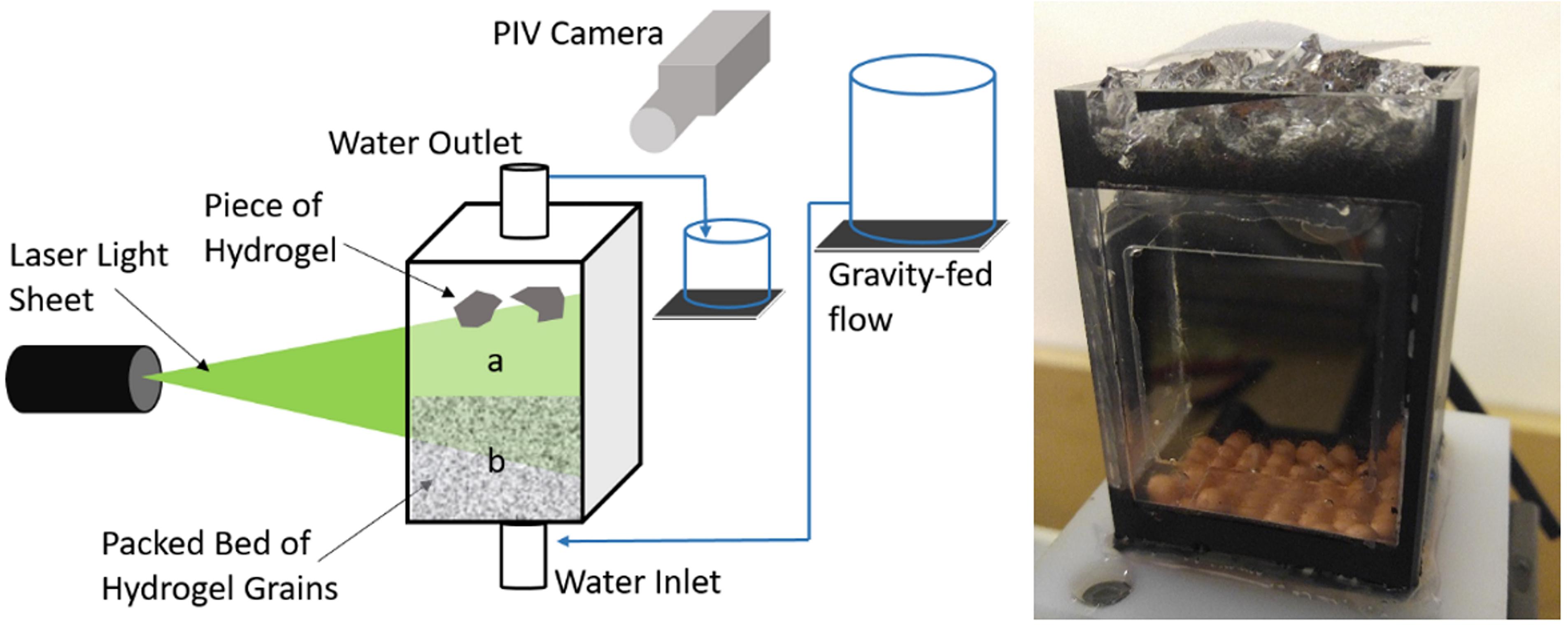
Figure 1. Flow cell schematic (on the left) operated in two modes: mode “a” with pieces of hydrogel, and mode “b” with a packed bed of hydrogel. Note that each mode was tested separately with only one mode being in the test cell at a time. The flow cell is 5 cm by 5 cm footprint and 7 cm high. Photograph of the flow cell (on the right) with the lid removed and filled with hydrogel grains and water. Additional hydrogel grains were added on the top and are in air. Those in the air are visible but those fully submerged are invisible in water as their refractive index matches that of the water.
Only one hydrogel piece (the left piece in Figure 2) for experiments (a) and all the hydrogel grains for the packed bed of experiments (b) were seeded with 4 μm Nylon particles. The seeding was conducted during the hydrogel fabrication process by dispersing the Nylon particles into a portion of the water used to form the hydrogel. Particle dispersion into the water was facilitated by placing the beaker of water on the tray of a water filled ultrasonic cleaner. Our intent was to have the second hydrogel piece (the right piece in Figure 2) to be completely unseeded for experiment (a), so we could make a comparison between seeded and unseeded solids. Thus, the hydrogel piece on the right-hand-side of the flow cell was not seeded intentionally, but, nevertheless, contained a sparse seeding of background particles present in the de-ionized water used to make the hydrogel. Degassed reverse osmosis filtered water was delivered to the test cell from a head tank to create water flow over the hydrogel pieces or through the packed bed.
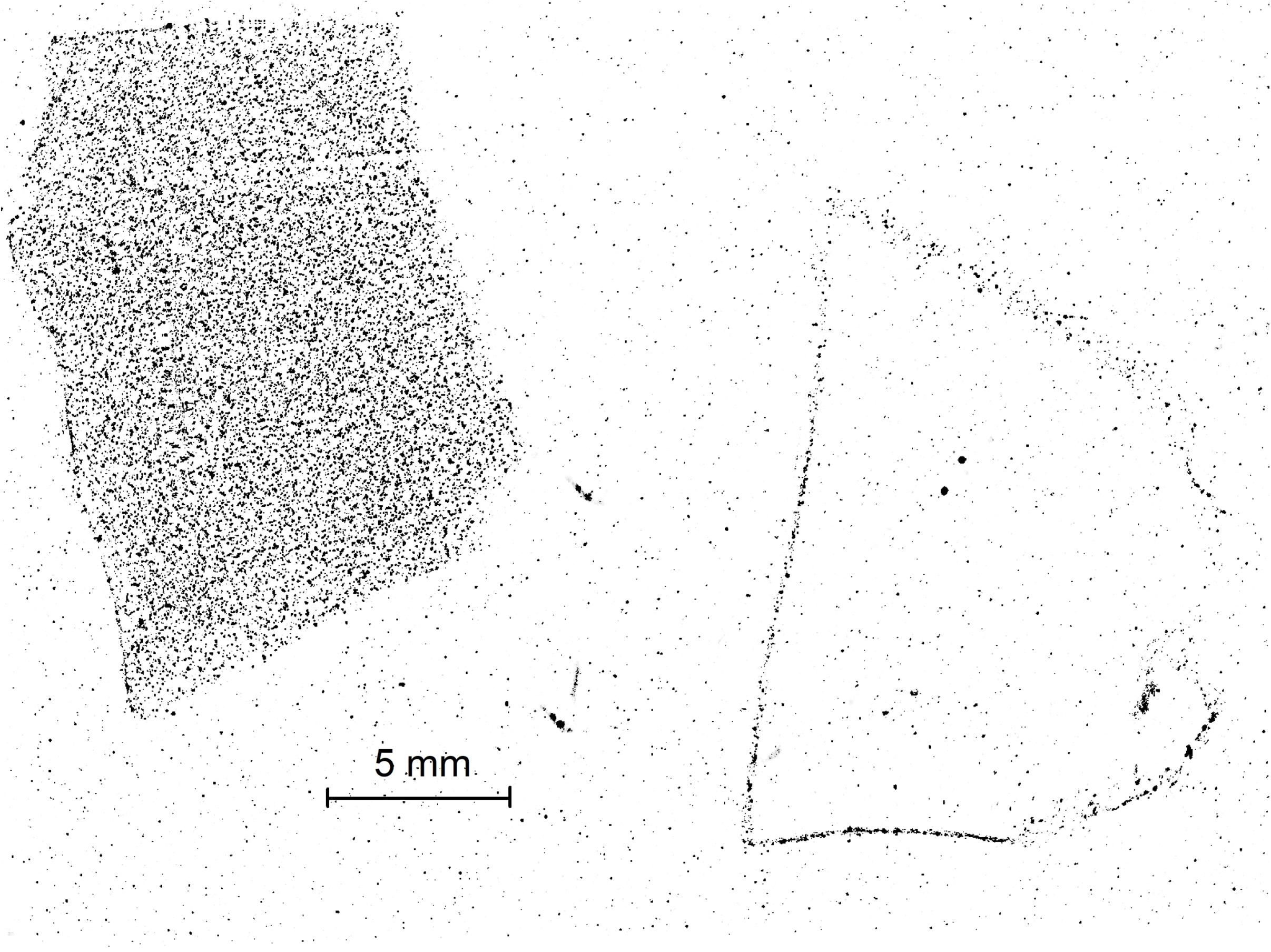
Figure 2. Image of hydrogel pieces in test cell for mode “a” experiment. The image of the piece on the left illustrates the potential for determination of the solid-liquid boundary by method 1, i.e., contrast between the heavily seeded grain and the lightly seeded fluid around the grain.
The PIV approach for this study used dual Nd:YAG lasers for light sheet production and a CCD camera with 1200 × 1600 pixels and a 180 mm focal length macro lens, which were required to obtain the field of view to capture the small flow passages among grains (interstitial flows). DaVis software was used for imaging and processing of the images. Image pairs were acquired at a rate of 3 pairs per second. Preprocessing of images included rotation and shift correction to diminish vibration effects as wells as subtraction of sliding average to reduce background noise. Image pairs were processed by a spatial correlation method down to a 12 × 12-pixel (0.11 mm × 0.11 mm) interrogation cell (IC) size. The only post processing conducted was outlier detection and removal.
The particle image velocimetry images and velocity results were then used to identify the fluid-solid boundaries by three methods, which may also be used in combination: (1) by contrast between seeded solid and unseeded fluid, (2) by applying a near zero-velocity threshold, and (3) by combining near zero-velocity with comparison between root mean square of the fluctuations of the in-plane velocity within the solid and the fluid.
Results and Discussion
Figures 2, 3 show the results for mode “a” experiments. Figure 2 shows the hydrogel pieces, which were rigidly held in place from behind (by two sewing needles inserted into each grain) and illuminated by the laser light sheet in the test cell as shown in Figure 1. The hydrogel piece on the left was seeded, whereas the piece on the right had only a background level of particles as described in section “Materials and Methods.” The water flowing around the pieces was not seeded but had background particles similar to the hydrogel piece on the right. Figures 2, 3 demonstrate that the solid material may be identified in the proposed three ways: (1) by contrast between seeded solid and unseeded fluid (Figure 2), (2) by applying a near zero-velocity threshold (Figure 3), and (3) by combining near-zero velocity with comparison between root mean square of the fluctuation of the in-plane velocity within the solid and the fluid. Whereas the first method does not require PIV but only light contrast between seeded solid and unseeded fluid, the last two methods require measurements of the velocity field and are based on the premises that (1) PIV predicted velocities within the solid are near-zero, and (2) because velocity in the solid does not change (stays near-zero) its temporal fluctuations are also near-zero.
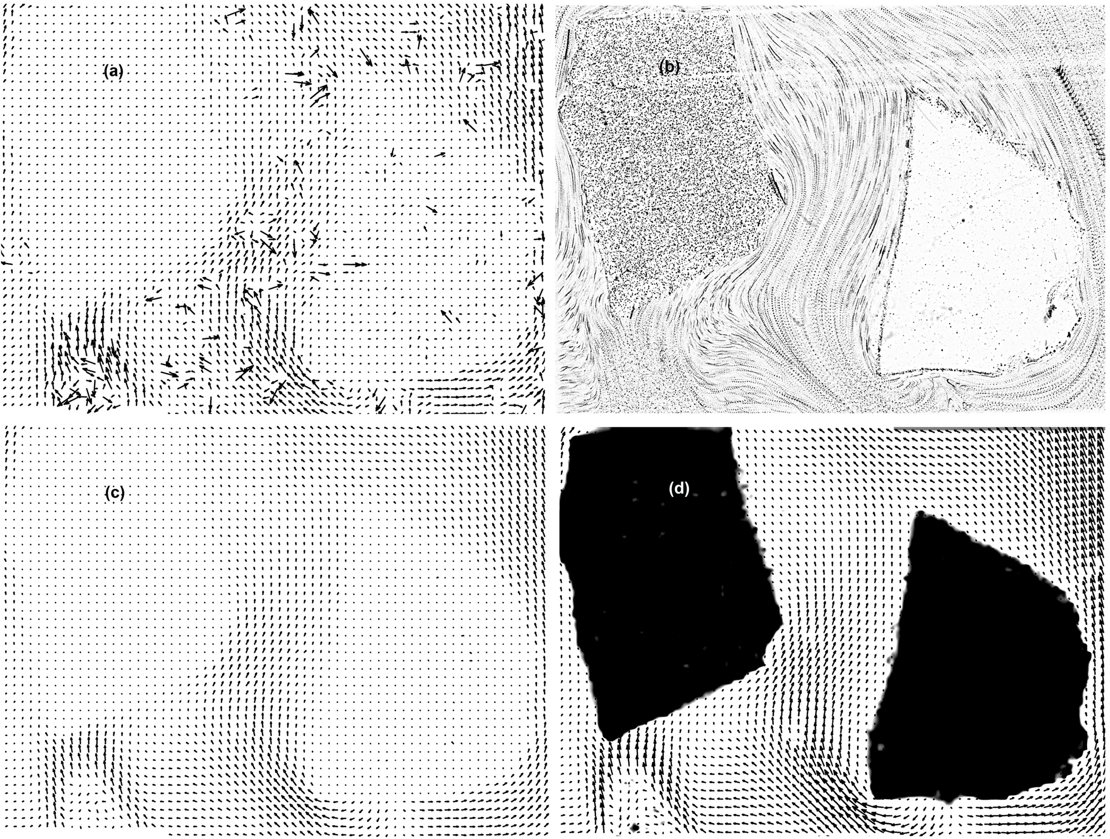
Figure 3. Flow around hydrogel pieces in test cell for mode “a” experiment. (a) Instantaneous vector field. (b) Time series showing particle-pathlines. (c) Average over 100 instantaneous fields. (d) Applying near zero velocity threshold to reveal outline of pieces (method 2 for finding the solid-liquid boundary). A velocity vector with length of one grid spacing had a velocity of 4.6 mm/s. The approximate vertical velocity in the cell away from the grains was 5 mm/s. All vector plots show a vector for every other interrogation cell (IC).
For the first method, the left piece of hydrogel was heavily seeded and was made distinct when immersed in lightly seeded fluid (Figure 2). The right solid piece has the same level of seeding as the fluid and normally would not be distinct, but the deposition of background particles on the surface of the hydrogel has defined the surface-fluid boundary over most of the perimeter of the hydrogel piece. Figure 2 also demonstrates that the laser light sheet illumination remained uniform even with the heavy particle seeding in the left piece of hydrogel.
For the second method, PIV was used to obtain the velocity field around the central plane of the hydrogel pieces including, instantaneous vector field (Figure 3a), time series showing particle-pathlines (Figure 3b), average over 100 instantaneous fields (Figure 3c), and applying near zero-velocity threshold to reveal the outline of pieces (Figure 3d). In addition, a video of the particle motion has been included in the Supplementary Video S1. The left solid piece in Figure 3a with dense seeding correctly shows zero-velocity vectors within the solid, while the right hydrogel piece with sparse seeding contains several spurious non-zero vectors, and which were not generated in seeded hydrogel because of the strong zero-velocity signal.
The outline of the pieces in the plane of the laser light sheet (i.e., the location of the fluid-solid boundary) may be determined by applying a near zero-velocity threshold to the PIV velocity results. Figure 3d shows the resulting piece outlines. The velocity threshold, vt, used to locate the boundary was 0.1 mm/s. All interrogation cells with velocity less than 0.1 mm/s were classified as solid and set to a black background color. This method also worked for the grain on the right since it had enough background seeding to provide zero velocity levels. However, this approach erroneously identifies as solid a small location in the flow field near the left bottom of the figure, a small black spot, because of its very low in-plane velocity.
To better constrain the near zero-velocity threshold method, we tested the third method to improve the ability to distinguish between solid material, and regions of low in-plane velocity. This method additionally uses the root-mean-square (rms) level of the in-plane velocity fluctuations to discriminate between solid and fluid. In the present flow, solid material had low rms levels and fluid had high rms levels. This will be the case for most flows with some level of unsteadiness due to instability or turbulence. For example, the rms level in the heavily seeded solid piece divided by the rms level of the fluid at the small black spot near the left bottom of Figure 3d had a ratio of 1 to 25. Thus, based on high rms level, the black spot at the left bottom of Figure 3d is actually fluid and it should be converted from solid (black color) to fluid (white color).
The velocity threshold, vt, of 0.1 mm/s was identified from the velocity distribution of the single grain experiment, mode “a” (Figure 4A, vertical dotted line). Both the frequency distribution, FD, (solid line) and the cumulative frequency distribution, CFD, (dashed line) show two groups of velocities. We classified the first group as slow velocities belonging to the seeds within the solid. The rms values also show an increase for values of velocities larger than vt (Figure 4C), as expected because rms for the fluid velocities should be larger than those of the solid. A similar behavior is visible in the rms of the velocity for the packed bed experiment, mode “b” (Figure 4D), with rms increasing beyond the vt threshold. However, the velocity CDF is smooth and does not show the bi-modal characteristic observed in mode “a” (Figure 4B), because of the large fraction of solid in the system. The selected vt is small enough to be near-zero velocity but large enough to have most of the low velocity points (Figure 4B). Some low velocities are actually slow moving fluid particles approaching the solid boundary. These slow moving fluid locations can be identified by their large rms, with rms values larger than twice the minimum rms value quantified in the solid (green triangle marker points in Figure 4D).
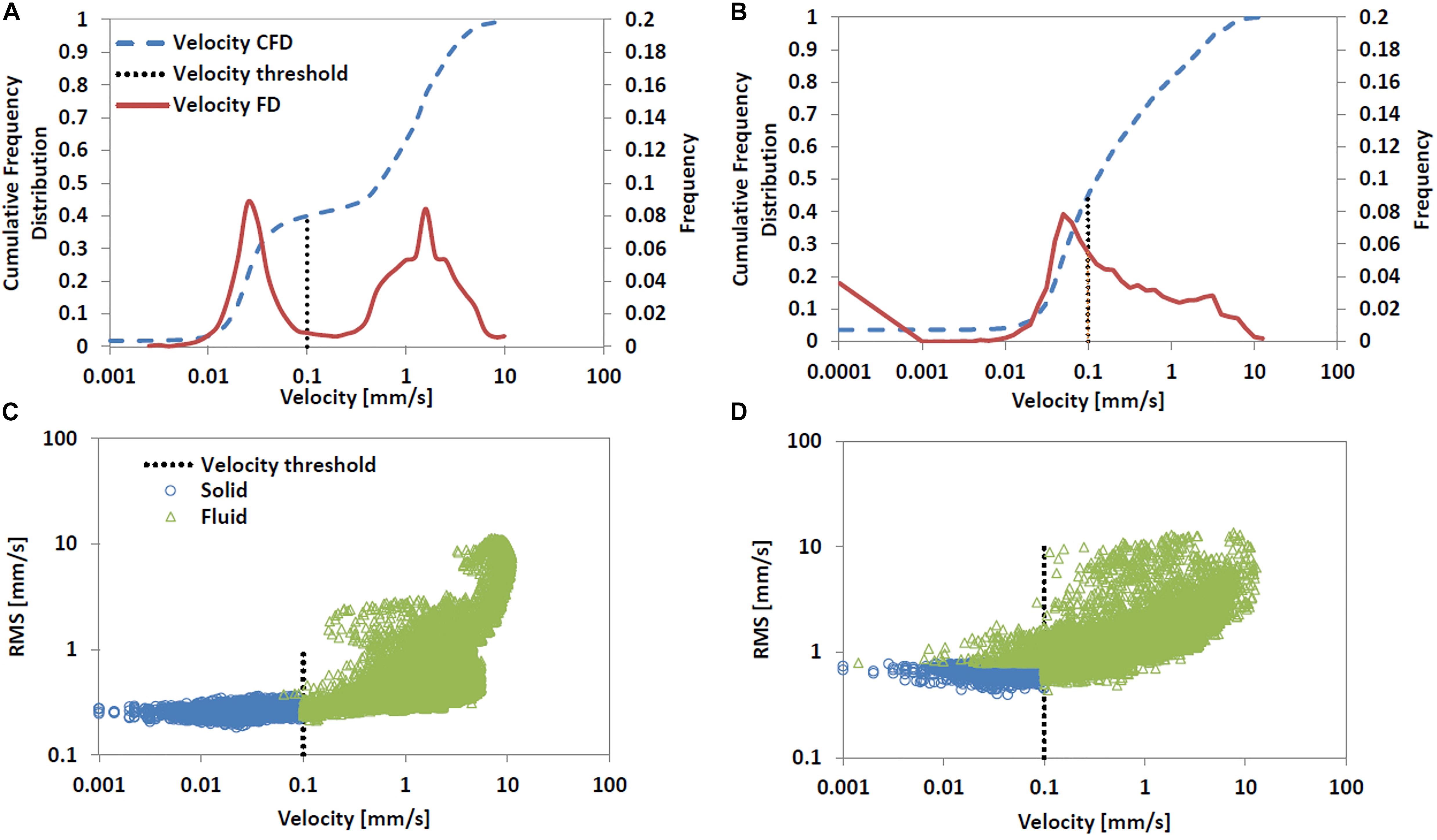
Figure 4. Cumulative frequency distribution, CFD, (dashed lines), and frequency distribution (solid line) of the entire velocity field including solid and fluid are shown in the upper graphs. The root mean square velocity levels (symbols) are shown in the lower graphs with blue points as solid and green points as fluid. Individual grain, mode “a” experiments, left graphs (A,C); and packed bed, mode “b” experiments, right graphs (B,D). The vertical dotted line identifies the velocity threshold of 0.1 mm/s that separates solid from fluid points. For the packed bed shown in (D), the threshold based on rms (twice the minimum rms, 0.39 mm/s) quantified several slow moving fluid locations that were below the velocity threshold. For the single grain shown in (C), the threshold based on rms (twice the minimum rms, 0.18 mm/s) quantified very few slow moving fluid locations and only closely adjacent to the velocity threshold.
Besides identifying the solid, the technique can help simultaneously quantifying and visualizing the flow field. The results of the time series particle pathlines reveal the flow patterns around the hydrogel pieces (Figure 3B). The flow at the top of the right piece appears to be emanating from the surface of the piece, which would violate the fluid, solid-surface boundary condition, and but it is an artifact of the three-dimensional characteristics of the flow. The reason for this apparently unphysical behavior is that the laser light sheet intersected the face of the hydrogel piece, where its face was strongly sloped upward, creating a significant vertical velocity component very near the surface. Nevertheless, the velocity went to zero at the hydrogel surface, as it must, to satisfy normal and tangential boundary conditions.
Regions with low magnitude in-plane velocity vectors were observed upstream of both pieces. The flow entered the cell through a small diameter inlet tube (Figure 1) without the aid of flow straighteners installed in the cell. This, along with the blocking effect of the two solid pieces, generated secondary flow patterns in the velocity field upstream of the pieces including out-of-plane velocities that were not resolved with the two dimensional PIV.
Flow velocities naturally approach zero velocity as the fluid gets closer to the boundary (the no-slip condition). These slow velocities may cause overestimates of the solid size. This effect was shown by comparing the digitized boundaries of the seeded grain identified by method (1) (Figure 5 solid red line) and by the combined method (2) and (3) (Figure 5 dashed blue line). Because of the highly irregular shape of the grain, we used the contrast method (1) to provide the reference size to compare that from the combined methods (2) and (3), because we can visually see the grain. The combined methods (2) and (3) yield an increase in the grain perimeter of 1.1% and in planar area of 2.8%. Most of the error is located near the downstream side of the grain were very low velocities of low rms fluctuations were formed. However, the overall error is small.
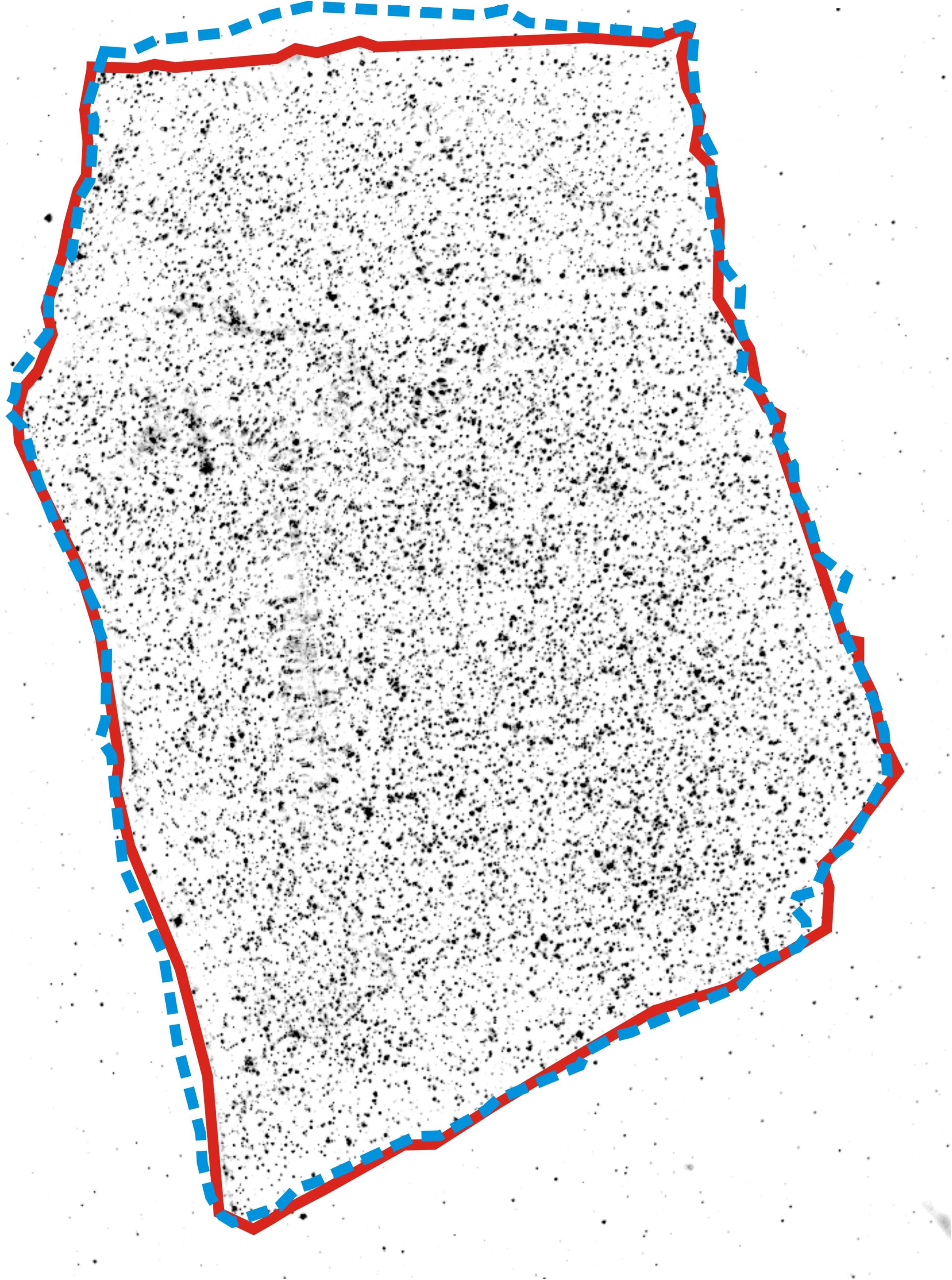
Figure 5. Boundaries of the seeded particle in mode “a” experiment identified based on method (1) by contrast with the surrounding fluid without particles, red solid line, and based on methods (2) and (3), which had similar results, blue dashed line.
The results for the mode “b” experiment with a seeded hydrogel packed bed are shown in Figure 6, which includes an instantaneous image of the seeding hydrogel grains infused with seeded flowing water (Figure 6a), a time series showing particle-pathlines (Figure 6b), and a plot with near-zero velocity threshold applied to reveal the outline of the hydrogel grains (Figure 6c). In addition, a video of the particle motion has been included in the Supplementary Video S2. The instantaneous image of particles shown in Figure 6a demonstrates that it is difficult to distinguish the location and extent of grains. We also took images of the seeded grains infused with reverse osmosis filtered water without added seeding. It was nevertheless difficult to distinguish the precise grain location and extent because of the presence of background particles in the filtered water. Thus, it would be impossible to apply the masking technique for this RIM packed bed study because the location and extent of the mask shape was unknown. The time series image shown in Figure 4B reveals stationary particles at grain locations and dark areas of particle-pathlines at locations where water was moving through the pore spaces. Pathlines moving around small solids or portions of large grains may appear to end in unconnected pores, which indicates a pathline has exited the plane, thus revealing a complex three-dimensional flow as water moves out of the plane through pores (Rubol et al., 2018).
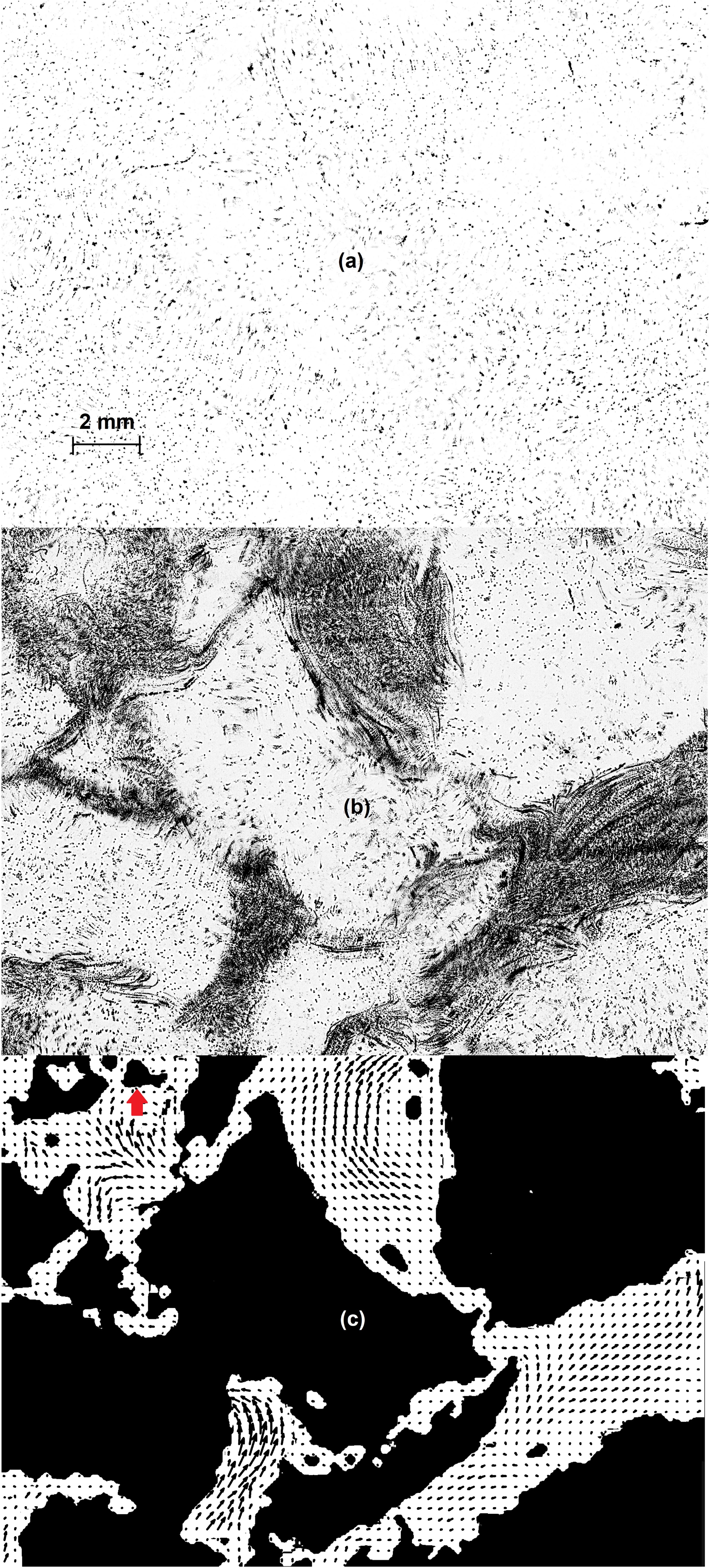
Figure 6. Flow through a packed bed of hydrogel grains. (a) Instantaneous image of particles. (b) Time series of particle motion. (c) Applying near zero-velocity threshold to reveal outline of grains (method 2 for finding the solid-liquid boundary). A velocity vector with length of one grid spacing had a velocity of 1.8 mm/s. The velocity in the interstitial spaces away from the boundary was 2 mm/s. The vector plot shows a vector for every fourth IC. Red arrows shows a solid identified by method (2), which instead should be a slow moving fluid when checked with rms value (method 3).
The in-plane pore water velocity vector plot (averaged over 100 instantaneous vector fields) is shown in Figure 6c along with blacked out interrogation cell’s (IC’s) at locations where the velocity was less than 0.1 mm/s. Velocity vectors in Figure 6c were plotted for every fourth IC and the scale was such that a velocity vector with length of one grid spacing had a velocity magnitude of 1.8 mm/s. The blacked out regions in Figure 6c reveal the extent of the grains in the plane of the laser light sheet. The image shown in Figure 6c is rich with details indicating the complexity of the pore spaces and multiple irregular grain shapes captured in the illuminated plane. The pore flow regions are in excellent agreement with the particle-pathline image shown in Figure 6b. The image in Figure 6c also reveals that pore spaces were small compared to regions of solid grain material (as it is typical because sediment porosity may range between 0.2 and 0.42), making it important to reduce the IC size to capture the details of the pore flow. The resolution of the present velocity threshold method used to determine the solid-liquid boundary location is set by the interrogation cell size. For the packed bed flow shown in Figure 4, the interrogation cell side length was 0.11 mm. We applied a smoothing function to interpolate velocity between neighboring interrogation cells.
We again tested the rms level method on the packed bed flow to better constrain the identification of solids. The method revealed that only one region was erroneously identified as solid but should have been slow moving fluid. This region was in the upper left area of the image and it is identified with a red arrow in Figure 6c. The ratio of the rms level of this region to the level within the seeded grains was 17 to 1, indicating that it was fluid rather than solid.
We were not able conduct a comparison of solid planar area between methods for mode “b” experiments, because the seeding level in fluid and solid were so close (see Figure 6a) such that it was impossible to distinguish between the two by method (1). Thus, the actual solid planar area of the irregular grains, as would be determined by method (1), was not available for comparison. Consequently, the mode “b” solid-liquid boundary results should be viewed as proof-of-concept. The primary method for identifying the solid-liquid boundary for a packed bed of irregular grains should be by contrast (method 1); since the flow over the packed bed of irregular grains is complex and this may affect threshold settings for methods (2) and (3).
Summary and Conclusion
In our test case, the seeded RIM grain was hydrogel and the fluid with matched refractive index was filtered pure water. The contrast between seeded grain and unseeded fluid was used to identify the solid-liquid boundary. The fluid was then seeded, allowing PIV analysis of the entire field of view regardless of the presence of fluid and solids (with no need to create a mask before performing PIV). In addition, the solid-liquid boundary was identified by considering locations with both near-zero velocity and low root mean square levels of the velocity fluctuations (i.e., low standard deviations of the velocity) in the field of view. Furthermore, the laser light sheet was not attenuated or distorted by seeding the RIM solid material and was able to uniformly illuminate the central plane of an entire packed bed of grains. We have also demonstrated that hydrogel may be fractured into grains for the study of packed bed flows. Other RIM liquid-solid pairs have the solid material with the potential for seeding as reported in Budwig (1994), Wiederseiner et al. (2011), and Wright et al. (2017). A likely candidate for solid seeding, in addition to the presently tested hydrogel, would be silicone rubber, which is paired with aqueous solution of sodium chloride and glycerol (Shuib et al., 2011). Others could be fluorinated ethylene propylene, FEP, or tetrafluoroethylene–hexafluoropropylene–vinylidene fluoride (THV), which, during three-dimensional (3D) printing, can be mixed with seeding. We believe that 3D printing, by both curing and melting techniques, will enable the proposed technique to be used with these and other solids. By curing method, the seeding can be mixed in the fluid and by melting process, the solid is shaped by applying the melted filament at micrometers thick layers, between which the seeding could be added (e.g., Guo et al., 2017).
The present seeded RIM solid approach is particularly attractive for irregular solid boundaries, like those found in packed beds. An a priori masking would be impossible for the present packed bed case and for any packed bed of irregular RIM grains. The present approach may be used to determine both the solid-liquid boundary as well as the velocity vector field. Additionally, by performing PIV in multiple planes across the test cell, the complete topography of the irregular grain packed bed as well as the pore flow map may be determined.
As in the work of Byron and Variano (2013), the method, in addition, could be used to identify the location of the solids and their motion. We also suggest, but we did not directly test it in this work, that the seeded RIM solid method is extremely powerful in studying moving mixtures of fluids and solid particles because the PIV spatial correlation analysis can be performed to the entire image regardless of where solids and fluid are. The mixture motion would be fully resolved. We suggest that the solid location and motion could be detected with pattern recognition analysis applied over several frames because the seeded RIM solid velocity field would follow that of a rigid body and would form a coherent structure. Thus, this physical modeling technique could be applied to other scientific fields beyond granular beds, such as flows within sediments and soils, and fluidized beds of mixture of fluid and particles. Other fields may include sediment transport, particle mobility analysis, and flow field around rough boundary like streambeds.
The ability to use irregular shaped grains of different sizes from fractions of a millimeter to centimeter sizes is significant, because these grains may be fabricated to mimic natural soil particles that are highly heterogeneous in sizes and shapes. Whereas masking is an effective technique when the shape and location of grains are known, it is not possible when grains have a range of unknown shapes and sizes. In the present study, we created and studied a packed bed of irregular grains, but we did not attempt to mimic the actual shape and size distributions of a real sediment bed, though there is the potential for this in future studies. Consequently, this technique provides an effective method for studying natural porous media flows, because it allows both the identification of the shape and size of the grains and the quantification of the flow field around them. This technique will pave the way to explore the interstitial processes within a simulated sediment bed, such as those of aquifers, soils, sediments, and the hyporheic zone (Tonina, 2012).
Author Contributions
WB, RB, and DT designed the experiments. WB and RB conducted the experiments and analyzed the data. RB and DT wrote the manuscript. WB reviewed the manuscript. All authors discussed the results.
Funding
This research was funded by the National Science Foundation award number EAR1559348. Any opinions, conclusions, or recommendations expressed in this article are those of the authors and do not necessarily reflect the views of the supporting agency.
Conflict of Interest Statement
The authors declare that the research was conducted in the absence of any commercial or financial relationships that could be construed as a potential conflict of interest.
Acknowledgments
We thank the three reviewers and the Associate Editor Theresa Plume for their valuable and insightful comments, which improve our contribution.
Supplementary Material
The Supplementary Material for this article can be found online at: https://www.frontiersin.org/articles/10.3389/feart.2019.00195/full#supplementary-material
Two video files have been included showing seeding particle motion in a plane of the test cell, (i) over the two irregular hydrogel grains (mode “a” experiment), and (ii) through the packed bed of hydrogel grains (mode “b” experiment). The original PIV image frames have been placed in the Hydroshare archive (Basham et al., 2019).
References
Adrian, R., and Westerweel, J. (2011). Particle Image Velocimetry. New York, NJ: Cambridge, 404–405.
Arthur, J., Ruth, D., and Tachie, M. (2009). PIV measurements of flow through a model porous medium with varying boundary conditions. J. Fluid Mech. 629, 343–374. doi: 10.1017/s0022112009006405
Basham, W., Budwig, R., and Tonina, D. (2019). Data for particle seeded grains to identify highly irregular solid boundaries and simplify PIV measurements. HydroShare. doi: 10.4211/hs.1f0242ee442945ca87de348ad2dd4315
Bellani, G., Byron, M., Collignon, A., Meyer, C., and Variano, E. (2012). Shape effects on turbulent modulation by large nearly neutrally buoyant particles. J. Fluid Mech. 712, 41–60. doi: 10.1017/jfm.2012.393
Budwig, R. (1994). Refractive index matching methods for liquid flow investigations. Exp. Fluids 17, 350–355. doi: 10.1007/bf01874416
Byron, M., and Variano, E. (2013). Refractive-index-matched hydrogel materials for measuring flow-structure interactions. Exp. Fluids 54, 1456–1461.
Dijksman, J., Brodu, N., and Behringer, R. (2017). Refractive index matched scanning and detection of soft particles. Rev. Sci. Instrum. 88:051807. doi: 10.1063/1.4983047
Fujita, I., Muste, M., and Kruger, A. (1997). Large-scale particle image velocimetry for flow analysis in hydraulic engineering applications. J. Hydraul. Res. 36, 397–414. doi: 10.1080/00221689809498626
Gui, L., Wereley, S., and Kim, Y. (2003). Advances and applications of the digital mask technique in particle image velocimetry experiments. Meas. Sci. Technol. 14, 1820–1828. doi: 10.1088/0957-0233/14/10/312
Guo, T., Lembong, J., Zhang, L. G., and Fisher, J. P. (2017). Three-dimensional printing articular cartilage: recapitulating the complexity of native tissue. Tissue Eng. Part B 23, 225–236. doi: 10.1089/ten.TEB.2016.0316
Harshani, H., Galindo-Torres, S., Scheuermann, A., and Muhlhaus, H. (2017). Experimental study of porous media flow using hydro-gel beads and LED based PIV. Meas. Sci. Technol. 28:015902. doi: 10.1088/1361-6501/28/1/015902
Hassan, Y., and Dominguez-Ontiveros, E. (2008). Flow visualization in a pebble bed reactor experiment using PIV and refractive index matching techniques. Nuclear Eng. Des. 238, 3080–3085. doi: 10.1016/j.nucengdes.2008.01.027
Kakani, K., and Dabiri, J. (2008). In situ field measurements of aquatic animal-fluid interactions using a self-contained underwater velocimetry apparatus (SCUVA). Limnol. Oceanogr. Methods 6, 162–171. doi: 10.4319/lom.2008.6.162
Kakani, K., Sherlock, R., Sherman, A., and Robison, B. (2017). New technology reveals the role of giant larvaceans in oceanic carbon cycling. Sci. Adv. 3:e1602374. doi: 10.1126/sciadv.1602374
Menter, P. (2016). Acrylimide Polymerization – a Practical Approach. Bio-Rad Laboratories, Tech Note 1156. Available at: http://www.bio-rad.com/webroot/web/pdf/lsr/literature/Bulletin_1156.pdf (accessed October 24, 2018).
Muste, M., Fujita, I., and Hauet, A. (2008). Large-scale particle image velocimetry for measurements in the riverine environment. Water Resour. Res. 44:W00D19. doi: 10.1029/2008WR006950
Rubol, S., Tonina, D., Vincent, L., Sohm, J., Basham, W., Budwig, R., et al. (2018). Seeing through porous media: an experimental study for unveiling interstitial flows. Hydrol. Process. 32, 402–407. doi: 10.1002/hyp.11425
Satake, S., Aoyagi, Y., Unno, N., Yuki, K., Seki, Y., and Enoeda, M. (2015). Three-dimensional flow measurement of a water flow in a sphere-packed pipe by digital holographic PTV. Fusion Eng. Des. 9, 1864–1867. doi: 10.1016/j.fusengdes.2015.03.023
Shuib, A., Hoskins, P., and Easson, W. (2011). Experimental investigation of particle distribution in a flow through a stenosed artery. J. Mech. Sci. Technol. 25, 357–364. doi: 10.1007/s12206-010-1232-4
Tauro, F., Porfiri, M., and Grimaldi, S. (2016). Surface flow measurements from drones. J. Hydrol. 540, 240–245. doi: 10.1098/rsif.2014.1283
Tonina, D. (2012). Surface water and streambed sediment interaction: the hyporheic exchange, in Fluid Mechanics of Environmental Interfaces, (eds.) Gualtieri, C. and Mihailoviæ, D.T. London: CRC Press, 255–294. doi: 10.1201/b13079-13
Weitzman, J., Samuel, L., Craig, A., Zeller, R., Monismith, S., and Koseff, J. (2014). On the use of refractive-index-matched hydrogel for fluid velocity measurement within and around geometrically complex solid obstructions. Exp. Fluids 55, 1862–1873.
Wiederseiner, S., Andreini, N., Epely-Chauvin, G., and Ancey, C. (2011). Refractive-index and density matching in concentrated particle suspensions: a review. Exp. Fluids 50, 1183–1206. doi: 10.1007/s00348-010-0996-8
Keywords: fluid-solid boundaries, hydrogel, hyporheic flow, irregular granular particles, PIV, porous media flow, refractive index matching
Citation: Basham W, Budwig R and Tonina D (2019) Particle Seeded Grains to Identify Highly Irregular Solid Boundaries and Simplify PIV Measurements. Front. Earth Sci. 7:195. doi: 10.3389/feart.2019.00195
Received: 31 October 2018; Accepted: 11 July 2019;
Published: 31 July 2019.
Edited by:
Theresa Blume, German Research Centre for Geosciences, GermanyReviewed by:
Flavia Tauro, Università degli Studi della Tuscia, ItalyRolf Hut, Delft University of Technology, Netherlands
Salvatore Manfreda, University of Basilicata, Italy
Copyright © 2019 Basham, Budwig and Tonina. This is an open-access article distributed under the terms of the Creative Commons Attribution License (CC BY). The use, distribution or reproduction in other forums is permitted, provided the original author(s) and the copyright owner(s) are credited and that the original publication in this journal is cited, in accordance with accepted academic practice. No use, distribution or reproduction is permitted which does not comply with these terms.
*Correspondence: Ralph Budwig, cmJ1ZHdpZ0B1aWRhaG8uZWR1