Hydroacoustic, Meteorologic and Seismic Observations of the 2016 Nansen Ice Shelf Calving Event and Iceberg Formation

On April 7, 2016 the Nansen ice shelf (NIS) front calved into two icebergs, the first large-scale calving event in >30 years. Three hydrophone moorings were deployed seaward of the NIS in December 2015 and over the following months recorded hundreds of short duration, broadband (10–400 Hz) cryogenic signals, likely caused by fracturing of the ice shelf. The majority of these icequakes occurred between January and early March 2016, several weeks prior to the calving observed by satellite on April 7. Barometric pressure and wind speed records show the day the icebergs drifted from the NIS coincided with the largest low-pressure storm system recorded in the previous 7 months. A nearby seismic station also shows an increase in low-frequency energy, harmonic tremor, and microseisms on April 7. Our interpretation is the northern segment of the NIS leading edge broke free during mid-January to February, producing high acoustic energy, but the icebergs remained stationary until a strong low-pressure system with high winds freed the icebergs. As the unpinning of Antarctic ice shelves is not a well-documented process, our observations show that storm systems may play an under-appreciated role in Antarctic ice shelf break-up.

Introduction

The Southern Ocean adjacent to Antarctica is changing, where Circumpolar Deep Water has been warming and moving up onto the continental shelf of Antarctica over the last 40 years resulting in an increase in ice sheet melting rates (Schmidtko et al., 2014). This ocean warming has led to Antarctic ice shelf break-up and iceberg formation becoming more common because of longer melting seasons, development of larger melt ponds, and enhanced basal melting, all of which can lead to crevasse growth and enhanced fracturing and break-up of ice shelves (Scambos et al., 2000; MacAyeal et al., 2003; Banwell et al., 2013). Destruction of ice shelves can also lead to inland glacier ice-flow accelerations which directly affect the Antarctic ice mass balance and global sea levels (De Angelis and Skvarca, 2003). Once icebergs are created by shelf break-up, they can have a significant impact on marine ecosystems because of their size and momentum. Icebergs can be enormous objects (tens of kilometers long) that carve huge troughs in the seafloor, while at the same time generating extremely high-energy acoustic waves capable of propagating over thousands of kilometers (Talandier et al., 2006). The sound energy from ice shelf break-up and iceberg grounding can significantly alter ambient ocean sound levels in Antarctica, directly impacting marine animals that use sound to communicate, navigate, and find food in their polar environment (Haver et al., 2018).

Seismo-acoustic signals generated by the breakup of ice shelves and iceberg formation, the focus of the study presented here, can have a wide range of potential source mechanisms. An extensive review of this literature is provided by Podolskiy and Walter (2016), but to briefly summarize, possible sources can include rifting, near surface crevassing and calving within and at the edge of the shelf, stick-slip motion/rupture of the ice-bedrock interface at the glacier base and pinpoints, collision and sliding between two adjacent ice masses, ice shelf flexure due to ocean tides and waves, as well as grounding and stick-slip motion on the seafloor. Indeed, iceberg collision, grounding and breakup have been shown to generate energetic hydroacoustic harmonic tremor as well as cryogenic icequake events detected both by in situ seismometers (MacAyeal et al., 2008) and hydrophones at distances of 10^1-3 km from the iceberg source (Talandier et al., 2002; Chapp et al., 2005; Royer et al., 2015).

Discrete cryogenic events (icequakes) and ice-related tremor have also long been observed in seismic research of glaciers on land, where signal characteristics range from small, high-frequency (10 Hz–1 kHz) events caused by crevasse formation at the glacier’s surface (Neave and Savage, 1970), to low frequency (<2 Hz) events caused by large icebergs that break off the glacier (Qamar, 1988). More recently, Walter et al. (2010) found a decrease in the number of low frequency seismic signals (in the 1–3 Hz and 10–20 Hz bands) associated with the transition from grounding to floatation of the Columbia Glacier (Alaska). This is analogous to ice shelf behavior, where upon flotation, the basal shear becomes small and stress perturbations exist only at the glacier margins. Also, an important process involved in iceberg calving at ice shelves is propagation of shelf penetrating fractures, or rifts (Heeszel et al., 2014). Seismic studies have also found that ice shelf rift propagation occurs through shallow (<50 m), small icequakes (moment magnitude or Mw > –2.0) that occur episodically in swarms of events near the rift tip that last for hours, but can also extend several kilometers back along the rift axis (Bassis et al., 2008; Heeszel et al., 2014). Lastly, glacierized fjords can also exhibit a peak in ocean sound levels in the 1–3 kHz range due to air bubbles that are released underwater by the melting ice (Pettit et al., 2015).

The Nansen Ice Shelf and 2016 Calving Event

The Nansen ice shelf (NIS) is located along the western Ross Sea in Victoria Land, East Antarctica. The NIS is formed by the adjacent flow of the Reeves and Priestley outlet glaciers (Frezzotti and Mabin, 1994), where its northern boundary abuts the Drygalski ice tongue (DIT) (Figures 1A,B; Khazendar et al., 2001). The NIS is ∼2000 km² in area, 200 m thick, with an average ice flow of 0.15 km year^-1 (Dow et al., 2018). The adjacent DIT is ∼75 km in length and is the ice shelf of the David Glacier, which has flow speeds ranging from 0.2 to 0.6 km year^-1 (Frezzotti and Mabin, 1994). The NIS has persisted throughout the warming period of the late Holocene era, advancing after ∼5,800 years b.p. to its present extent (Hall, 2009). The NIS is thought to be pinned on multi-year ice near the DIT to the south, and on a topographic high (Inexpressible Island) to the north (Dow et al., 2018; Figures 1C,D).

FIGURE 1

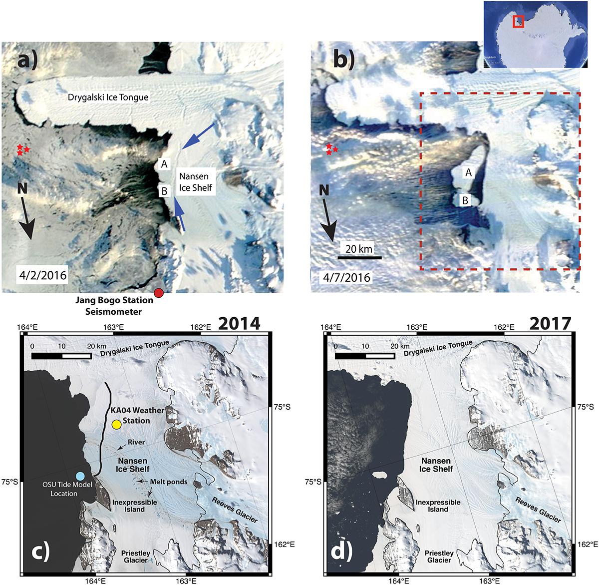
Figure 1. Diagrams show satellite images of DIT and NIS in the western Ross Sea. (a) Blue arrows highlight fracture in NIS on the days leading up to calving event on 7 April, shown in panel (b). Iceberg “A” is C33, iceberg “B” is the unnamed iceberg referred to in text. Red stars are locations of NOAA/PMEL hydrophone moorings, red circle shows location of seismometer at Jang Bogo Antarctic Station (Figure 6). Images in panels (a) and (b) are from NASA MODIS (blogs.agu.org, courtesy M. Pelto), North is oriented downward as shown by arrows. (b) Top right inset map shows location of satellite images in western Ross Sea, Antarctica. Red box shows approximate area covered by images in panels (c) and (d). (c) Landsat-8 image of NIS from January 2, 2014. Thick black line shows the 2016 calving front, thin black line is the grounding line (e.g., Dow et al., 2018). Yellow circle shows location of weather station KA04, which provided meteorological data in Figure 5. Blue circle is location used to estimate ocean tides utilizing Oregon State University (OSU) tide model (Figure 5B). (d) Landsat-8 image of NIS from December 2017, after 2016 calving event.

Satellite imagery from April 7, 2016 (Figure 1) showed the front of the NIS disintegrated into two medium-sized icebergs, the largest was C33 (153 km²), while the other was unnamed (61 km²). The total calving area was ∼214 km² with an average thickness of 200 m and a mass loss of ∼37 Gt (Li et al., 2016). The calving event occurred along a rift that was first observed by Landsat imagery in 1987, located ∼6.5 km from the coastline, and progressively grew at an accelerating rate. The crevasse width expanded substantially during 2013–2016 due to ocean currents, wind stress, hydraulic pressure (Li et al., 2016), and surface meltwater (Bell et al., 2017). The fracture had reached 40 km in length by April 6, 2016, extending from its north and south pinpoints (Dow et al., 2018). As of April 2, the satellite images showed that the leading edge of the shelf, seaward of the fracture, remained near or even possibly still attached, but then had separated by April 7. The 2016 NIS calving event is also thought to be the result of shelf fracture driven by channelized thinning, as several Antarctic ice shelves have also exhibited thinning and weakening due to warm ocean water entering into cavities underneath the shelves (Dow et al., 2018). After calving, the two icebergs were driven by winds and currents and drifted northward along the Terra Nova Bay (TNB) coastline, drifting out of TNB during the end of 2016 (Bell et al., 2017).

The goal of the experiment presented in this paper was to deploy a triad array of moored hydrophones in the western Ross Sea to record the short-duration hydroacoustic signals of ice-cracking and break-up (in the 10–400 Hz band) associated with the ice shelves in the region. Deployment and recovery of this Ross Sea hydrophone array was a collaborative effort between the NOAA/Pacific Marine Environmental Laboratory and the Korea Polar Research Institute. The temporal overlap of the hydrophone deployment with the 2016 NIS calving event has thus presented a rare opportunity to study cryogenic signals and ocean ambient sounds before, during and after a large-scale ice shelf calving and iceberg formation event.

Instrumentation, Data Analysis and Methodology

Passive Acoustic Recording System and Mooring

In December 2015, an array of three hydrophone moorings was deployed near the northeastern edge of the DIT (Figures 1A,B), with an equilateral triangle array geometry (∼2 km per side) to facilitate estimating the bearing (back azimuths) to acoustic sources detected in the region. All three of the hydrophone moorings were recovered in February 2017 having recorded 14 months of continuous, broadband acoustic data. The acoustic recording package used here is autonomous, and consists of a single ceramic hydrophone, with a filter/amplifier, clock, and a low-power processor, all powered by an internal battery pack. The instrument records at 1 kHz sample rate at 16-bit data resolution for 1 year, designed to record low frequency (typically < 500 Hz) cryogenic acoustic signals (e.g., Dziak et al., 2018). The hydrophone is an ITC-1032, which is omni-directional with a response of –194 dB re 1 V μPa^-1. The pre-amplifier has an 8-pole anti-aliasing filter and was designed to equalize the spectrum, over the pass band, against ocean noise. The pre-amp gain is designed to pre-whiten for typical deep-ocean noise due to light-moderate ship traffic, as well as a sea state of 1 to 2, as defined by the Wenz curves (Wenz, 1962). For this study, we used a gain curve setting of 8 dB at 1 Hz, 38 dB at 10 Hz, 43 dB at 100 Hz, and 55 dB at 800 Hz. The clock used is Cesium atomic (low power) with an average time drift of ∼0.1 s year^-1, providing accurate timing for this 1 year deployment duration.

The electronics were housed in a fiberglass composite pressure case attached to a standard oceanographic mooring with an anchor, acoustic release, mooring line, and syntactic foam float designed to place the sensor at a depth of 400 m. The 400 m depth was chosen because it should place the mooring below the keel depth of nearby icebergs. Sound speed profiles were sampled in the western Ross Sea by the Research Vessel Araon in 2015 and 2018, and indicate the water-column sound propagation field is surface limited. Although a duct forms at 100 m depth during austral summer, this duct is no longer present in austral autumn (Figure 2). Thus both the relatively close distance (∼60 km) of the hydrophones from the NIS, and their depth in the water-column, should allow for a good recording of the shallow-water sound-propagation of cryogenic signals sourced from the NIS (Dziak et al., 2018).

FIGURE 2

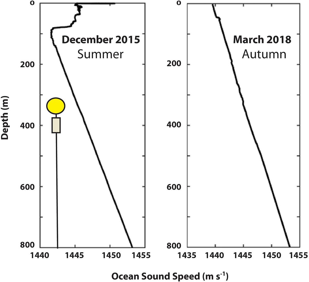
Figure 2. Sound velocity profiles from the Ross Sea, sampled near northernmost hydrophone mooring (Figure 1). Profiles calculated using conductivity, temperature and depth (CTD) measurements from the South Korean Research Vessel Araon in December 2015 (austral summer, left) and March 2018 (austral autumn, right). Sound velocity estimates from CTD data are based on the algorithms of Chen and Millero (1977), and Seasoft V2 data processing software (https://www.seabird.com). Schematic of the hydrophone mooring is shown on the left, with a float (yellow circle) and a hydrophone instrument demonstrating the depth of the hydrophone in relation to the sound profiles.

Ice Shelf Acoustic Signal Observations

Hydrophone data from the terminus of the DIT was converted to a spectrogram and is shown in Figure 3A. The record here covers the time range from January 1 to May 1, 2016, which includes the April NIT iceberg formation event. The spectrogram shows that there are hundreds of broadband signals throughout the 4-month hydrophone record. We interpret these signals as likely cryogenic, caused by the cracking of the ice shelves and impacts of nearby sea-ice. These icequakes and ice-related signals recorded by the moored hydrophones are wide-band (∼10–400 Hz) events, with durations of ∼10–30 s. The cryogenic signals, or icequakes, can be distinguished from earthquakes on the hydroacoustic record by the lack of crustal phase arrivals (P- and S-waves) and low frequency energy (<10 Hz). We interpret the lack of low frequency (<10 Hz) energy as possibly caused by a combination of (1) the icequake fracture planes are relatively small in area, and are unable to produce the low frequency signals of earthquakes, (2) the water depth (800 m) and sound speed (∼1445 m s^-1) at the moorings limit sound wavelengths to >2 Hz, and (3) the hydrophone filter begins to roll-off under 5 Hz. Moreover, the presence of relatively high (>100 Hz) frequency energy in the icequake signals (Figures 3B,C) is consistent with these cryogenic sources being relatively close to the hydrophones (tens of kilometers). The icequakes may also even be above the sea surface, but the surface limited sound speed profile may still reduce high frequency attenuation.

FIGURE 3

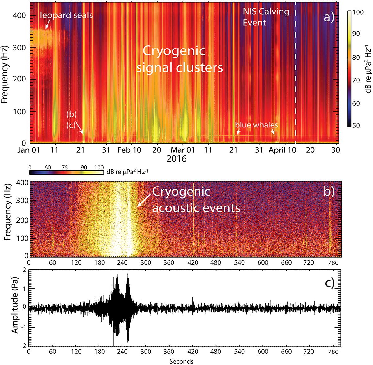
Figure 3. (a) Spectrogram of 4 months of hydrophone data from the western-most of the three Ross Sea hydrophones. Significant cryogenic activity (icequakes and ice-related rifting) can be seen as high energy (yellow), broadband (∼10–400 Hz) acoustic energy during February–early March 2016, 1 month prior to the NIS calving event on April 7 (white dashed line). Vocalizations of leopard seals, blue whales and time of hydrophone data shown in panels (b) and (c) are also labeled. (b) Spectrogram and (c) time series showing examples of two strong cryogenic events recorded on the hydrophone triad. Amplitude of time series in units of Pascals (Pa). Figure shows 13 min of data from January 22, 00:18 to 00:31. Several impulsive, short duration ice-cracking events are also on the record.

To derive counts of icequakes, we implemented the beam-forming algorithm described in Haney et al. (2018) on the hydrophone triad records, where delay times Δt between the three elements of the array are computed with cross correlations over successive time windows of 45 s length with 6 s overlap. A received signal is counted as a detection when the maximum of the normalized cross correlation exceeds a minimum value of 0.2 for signal pairs of the three elements of the array. A 30–50 Hz passband was chosen to avoid the earthquake T-phase frequencies at 1–25 Hz as well as the marine mammal vocalization frequencies at 300–350 Hz and 28 Hz (Širović et al., 2004; Opzeeland et al., 2010). A total of 513 windows with correlation values in the range of 0.2 to 0.7 (indicating moderately correlated) were determined to have coherent energy across the triad array (Figure 4A). Given our choice of frequency band, and visual inspection of the records, our interpretation is these detections are icequakes and ice-related tremor. All but one of the detections occur during the January 1 to March 14 time frame.

FIGURE 4

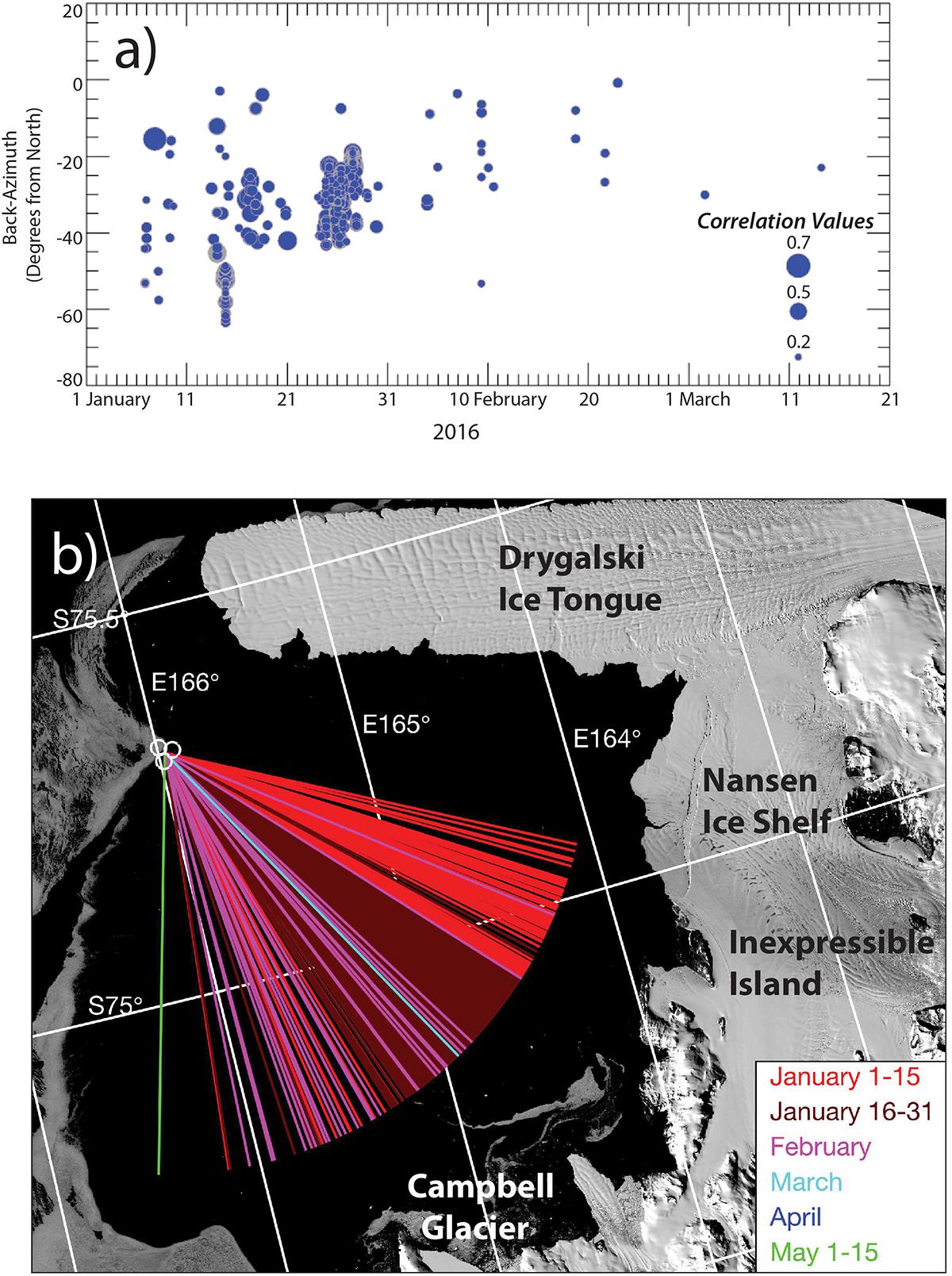
Figure 4. (a) Diagram showing the back azimuth and date of occurrence of cryogenic signal sources detected over the time period from January 1 to March 21, 2016. A total of 513 individual cryogenic sources were detected on the hydrophone triad during this time period. Circle size is scaled to coherence value of signals between hydrophones, with larger size relating to higher coherence value. Back azimuths fall within 0° to –65° relative to north. (b) Map view of back azimuth estimates, plotted on Landsat-8 image taken from February 2, 2016. Line segments show back azimuth direction from triad array location to cryogenic sources. Line colors designate time periods the sources were detected.

We also tested our detection algorithm at higher frequency bands (60–100 Hz and 100–200 Hz) where icequake sound appears prevalent; however, the shorter wavelengths at these frequencies are less coherent across the hydrophone array. There is also an increase in background noise in this frequency range (Figure 3A), and the detection algorithm was unable to resolve many discrete events. We interpret the increase in broadband, diffuse noise in these bands as due to low-pressure weather systems that passed through the area during this time period, significantly raising background sound levels. These low-pressure systems (storms) can elevate broadband energy (50–500 Hz) by increasing wind speeds (Wenz, 1962) which leads to increased wave heights as well as increased sea-ice impacts and break-up. It seems likely this increase in background noise levels decreases the coherence of the signal, by reducing signal to noise ratios, and may lead to fewer icequake detections than expected. Similar increases in high frequency background noise are also seen during March 21 and the calving event time period of April 6–11, when wind speed and ambient sound levels are at relative highs (Figure 5A).

FIGURE 5

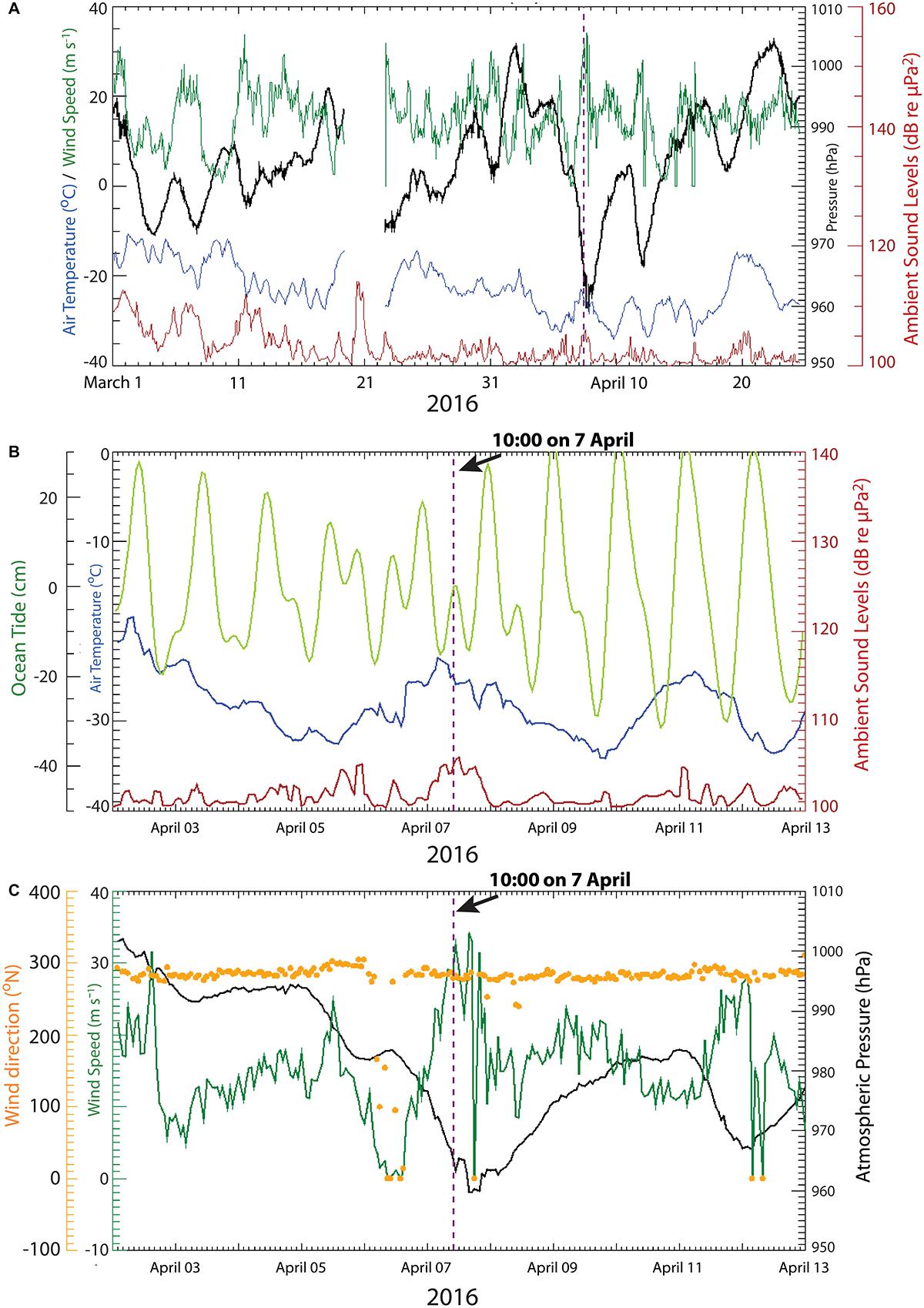
Figure 5. (A) March 1 to April 25, 2016 record of temperature (blue), wind speed (green), and atmospheric pressure (black) from weather station at Jang Bogo station, western Ross Sea (location in Figure 1C). Red line shows the ambient sound levels recorded by the hydrophones, estimated using the root-mean-square (RMS) amplitude of sound for every hour over the 24 h for each day of the recording period. (B) Diagram shows the air temperature, ocean tide height, and ambient sound levels several days before and after the NIS calving event. Ocean tide levels estimated using Oregon State University global tide predictor available at http://volkov.oce.orst.edu/tides/global.html. Location of tide estimate shown as blue circle in Figure 1C. Dashed line notes time of onset of low frequency energy recorded on a nearby seismometer at 10:00 UTC on April 7 (Figure 6). (C) Diagram showing wind speed, wind direction and atmospheric pressure over same time range as (B). Orange dots indicate wind direction, ranging from 0° (due North) to 360°.

The Haney et al. (2018) algorithm also estimates the direction from the triad array to the source of the detected signals, referred to as the back azimuth (Figures 4A,B). The delay times of signal pairs of the three array elements were inverted for the slowness vector of a plane wave traversing the array. Once the slowness vector is estimated, it is straightforward to obtain the back azimuth θ and trace velocity v of the plane wave. We estimated back azimuths for all 513 correlated acoustic signals detected by the hydrophone array, which resulted in a range of back azimuths between 0° and -65° relative to North (Figures 4A,B). The back azimuth estimates have standard deviations that range from 0.04° to 0.001°. Figure 4B shows the map view of the back azimuth estimates relative to the NIS and DIS. The back azimuths from January 1 to 15 are directed at the northern edge of the NIS, indicating ice-related signals were sourced, where the NIS was pinned at Inexpressible Island. The remaining back azimuths from late January to May indicate icequakes were sourced north of the Nansen toward the ocean entry of Campbell Glacier.

Lastly, we estimated the overall ambient acoustic energy, by calculating the root-mean-square (RMS) amplitude of ambient sound levels for every hour over the 24 h for each day of the recording period. The data from each hydrophone were low-pass filtered at 250 Hz and the instrument response was removed. The RMS for each hour was obtained using √(ΣA²/n), where A is the sound level amplitudes recorded within an hour, and n = number of data points in 1 h, or 3600 points given the sample rate of 1 kHz. We then converted these values to dB using dB = 20(log₁₀ (RMS)), and took the median of the three hydrophone values. It is this estimate we used to assess the long-term (weeks to months) variability in ambient sound levels of the region (Figure 5A). Interestingly, the acoustic energy levels were at a relative maximum level during the time period from January 19 to March 1 (seen as broadband energy in Figure 3A), with the period in late March through April being a relatively low acoustic energy level. The long-term acoustic energy shows a relative maximum throughout the day on April 7, reaching 106 dB re μPa which was the highest level within a 2 weeks period around the calving event (Figures 5A,B).

Meteorologic, Ocean-Tide, and Seismic Data Observations

To provide perspective on this apparent temporal discrepancy between the acoustic energy peak and satellite observed calving event, we reviewed the wind speeds, wind directions, barometric pressures, and air temperatures recorded for the region near the NIS in the western Ross Sea (Figures 5A–C). This meteorological data was collected by a Vaisala WXT52^TM weather station incorporated into an autonomous observation system located near the Jang Bogo station (Figure 1A; Scambos et al., 2013). The meteorological data shows that on April 7, the day iceberg C33 calved and flowed away from the NIS, the highest winds and the largest low atmospheric-pressure system recorded in the previous 7 months passed over the area (Figure 5A). Figure 5B shows the ocean tide near the NIS front using the Oregon State University ocean tide prediction model. The high and low tide estimates are provided at 1 h resolution, with high tide of +0.14 cm at 10:00 UTC (all times subsequently listed are UTC) and low tides of -15.2 cm and -14.0 cm at 05:00 and 16:00, respectively. Figure 5C shows atmospheric pressure decreased throughout the day on April 7, ending at a low of 959.6 hPa during the hour of 15:00–16:00. Wind speeds were a maximum (33.1 and 34.1 m s^-1) at the same time as maximum low pressure, with the first peak in wind speed occurring at ∼10:00. Winds were sourced from the west-northwest for almost all times of April 7, which is consistent with moving the icebergs away from the NIS. Temperature was a relative high during the low pressure event on April 7, reaching -22.9°C at 03:51.

We also reviewed the vertical component records of a seismometer at Jang Bogo Polar Base, located ∼30 km north-northeast of the NIS at 74.614°S; 164.214°E (station code JBG2). The seismometer is a Nanometrics Trillium Compact, with a sample rate of 100 Hz and flat response over the 0.01–40 Hz band. During April 7, a gradual increase in long-duration, low-frequency (<5 Hz) energy can be seen on the recording starting at ∼10:00, which continued on until 00:00 on April 8 (Figures 6A–C). During the time of increase in the low frequency energy, several episodes of harmonic tremor can also be seen in the spectra. The tremor signals are consistent in frequency and duration with tremor observed during iceberg collision and grounding (MacAyeal et al., 2008). Primary and secondary microseisms were also recorded, which are produced by the impact of ocean swells on the coastline (primary) and subsequent reflection/refraction (secondary) of these low frequency waves (Lee et al., 2011; Kanao et al., 2017). We were unable to calculate a back azimuth from this single seismic station to the source of the low-frequency signal. Interestingly, the P-wave and surface waves of a Mw 6.7 earthquake sourced at Vanuatu (27.6 km deep, epicentral distance ∼61°) can also be seen as high amplitude arrivals on the seismic record at 03:40, ∼6 h prior to the onset of the low frequency energy. However, there is no strong evidence to causally link these two events. Lastly, we reviewed the Jang Bogo seismometer data during early January to see if ice-related signals detected on the hydrophones, directed at the northern edge of the NIS, were also detected by the seismometer. The seismometer did not detect similar signals during this time period. We think this may be due to the frequency response of the seismometer (<5 Hz), which is too low to detect icequakes, which are higher frequency (∼10–400 Hz).

FIGURE 6

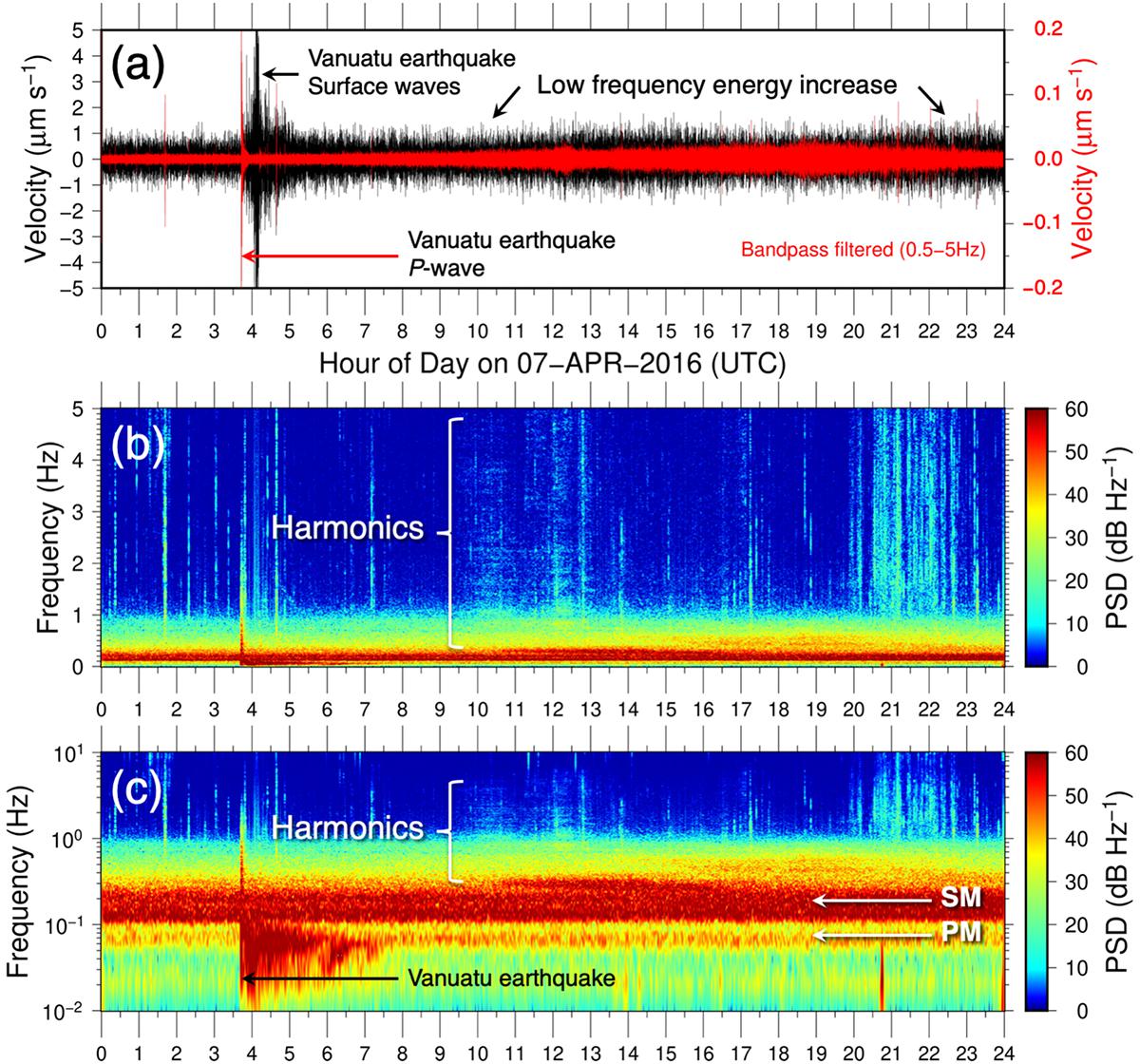
Figure 6. Diagram shows seismogram and corresponding spectrograms recorded by the vertical component of the seismic station at Jang Bogo Polar Base. (a) Unfiltered (black) and bandpass filtered (0.5–5 Hz; red) seismic data. The P-wave first arrival (red) followed by surface waves (black) from a Mw 6.7 Vanuatu earthquake are labeled. (b) Spectrogram showing low frequency energy distribution <5 Hz. Harmonic tremor observed in the spectrogram is labeled. PSD stands for power spectral density. (c) Shows a semi-logarithmic scale of the same spectrogram in panel (b) to enhance low frequency energy and harmonic signals. Primary (PM) and secondary (SM) microseism energy bands, as well as the Vanuatu earthquake, are labeled.

Interpretation

Although the unpinning of Antarctic ice-shelves is not a well-documented process (Favier et al., 2016), it is thought that unpinning can occur over various timescales due to progressive ice shelf thinning (Pritchard et al., 2012; Paolo et al., 2015), erosion, rising sea level, tidal uplift (Schmeltz et al., 2001), or through the developments of surface rifts (Humbert and Steinhage, 2011). Bassis et al. (2008) showed that as ice shelves thin, or as surface rift systems mature and iceberg detachment becomes imminent, short-term stress variations due to winds and ocean swell may become important factors affecting internal stress and balance of forces in the detaching part of the ice shelf. As a glacier transitions from a grounded terminus to a floating ice shelf, basal shear becomes small, and stress perturbations exist only at the shelf margins (Walter et al., 2010). Thus calving of the floating ice shelf terminus can be triggered by small-scale linkage of fractures, which can produce large icebergs despite a reduction in seismic (i.e., icequake) energy release during the fracturing and calving process (Walter et al., 2010).

Antarctic ice shelves have also been shown to respond mechanically to both ocean tides as well as tele-tsunamis and distantly generated ocean infragravity waves. Pirli et al. (2018) showed that rates and magnitudes of cryogenic earthquakes at the Fimbul Ice Shelf (East Antarctica) fluctuate steadily with the cycles of the ocean tide, showing correlations with tide height and spring tides as well as migration of icequakes landwards during the rising tide. Adalgeirsdottir et al. (2008) showed the basal seismicity and velocity of an Antarctic ice stream respond to tidal forcing as far as 40 km upstream. Thus ocean tides can have a mechanical influence on the flexure and fracture of an ice shelf. The tsunami from the Mw 9.1 2011 Honshu earthquake did cause calving of the Sulzberger Ice Shelf (Brunt et al., 2011), and infragravity waves have been shown to cause flexure of the Ross Ice Shelf (Bromirski et al., 2010). However, there was no Pacific basin scale tsunami at the time of the 2016 NIS event. It is also possible that infragravity waves may have contributed to the NIS calving event. We do not, however, have the data available to evaluate this possibility.

Our interpretation is that the NIS leading edge broke free during the January–March high hydroacoustic energy time period (Figures 7A–C) rather than the April 7, date when the icebergs were observed drifting out to sea away from the NIS using satellite imagery. The icequake back azimuths from early January, and several that occurred during February 2016, are directed at the northern edge of the NIS where the NIS was pinned at Inexpressible Island (Figure 4B). Thus it is our view that the mid-January to February icequakes were sourced at the northern part of the NIS, and it is possible this activity indicates the northern pinpoint at Inexpressible Island fractured and rifted apart during this time period (Figure 7B). The icebergs then apparently remained in place for months where they stayed juxtaposed with the DIT and Inexpressible Island, but did not become completely unmoored and break free until the low pressure event on April 7 (Figure 7C). The lack of back azimuths directed at the southern segment of the NIS, and its pinpoint with the DIT, is admittedly a bit surprising. We speculate that this lack of cryogenic activity indicates the southern section of the NIS may have remained pinned at the DIT until the April 7 meteorological event.

FIGURE 7

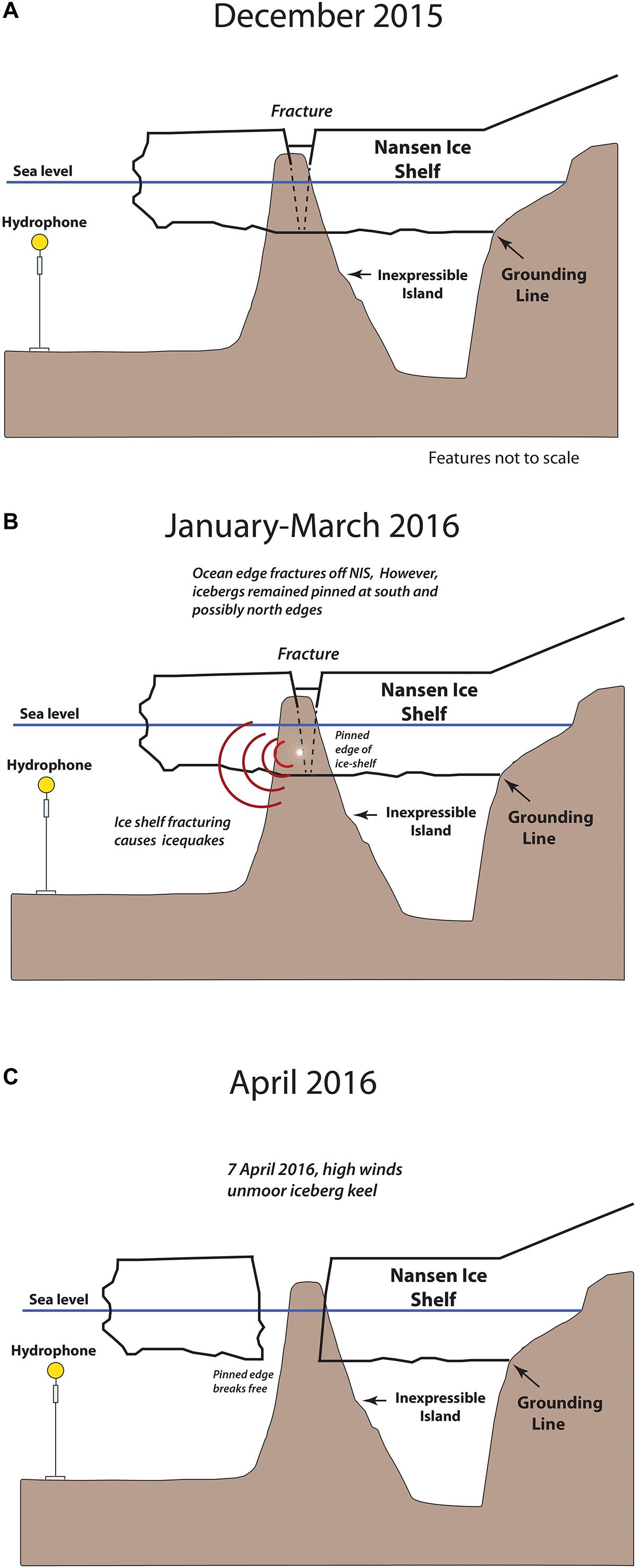
Figure 7. Illustrations showing interpreted sequence of NIS fracture and iceberg formation. (A) Represents month of December 2015, when a fracture is present within the NIS that was first observed in 1987. (B) Leading edge of NIS broke free during January–March 2016 time frame, however, ice shelf edges may have remained pinned on a topographic high (Inexpressible Island) to the north and by multi-year ice near the DIT to the south (Dow et al., 2018). (C) On April 7, 2016, a large storm (high winds, low pressure) freed icebergs.

As for the timing of the iceberg separation from the NIS, the nearby seismometer recorded the onset of low-frequency (<5 Hz) energy at ∼10:00 on April 7, that was accompanied by both harmonic tremor and microseisms (Figures 6A–C), and is the time of relatively high ocean acoustic energy (Figures 5A,B). The time of 10:00 also corresponds to the first maximum in wind speed (Figure 5C), suggesting the increase in low-frequency energy recorded by the seismometer could be a result of wind generated noise, likely due to increasing wind-induced ocean waves. However, wind and wave generated ocean noise are typically in a much higher frequency band (∼50–500 Hz; Wenz, 1962). Thus another possible explanation is that the increase of low frequency energy and harmonic tremor on the seismometer also marks the start of the icebergs breaking free (Figure 7C), colliding with the DIT and each other, then drifting into the Ross Sea, where the physical movement of the icebergs through the ocean can also cause a rise of low frequency seismo-acoustic energy (and possibly microseisms) detected on the seismometer. The high wind speeds are out of the north-northwest during this time period (Figure 5C), which may have helped force the icebergs ocean-ward, and may have aided in freeing the icebergs. The time of 10:00 also corresponds to the high tide level at the NIS, although the high tide is relatively low on April 7 as compared to other high tides just a few days before or after (Figure 5B). Therefore it is unclear what effect the high tide level may have had on freeing the icebergs. However, it is also possible the microseisms recorded were produced by incoming ocean swells, and along with the high tide, could have played a role in unmooring the icebergs.

Thus there appears to be a good temporal correlation of the seismo-acoustic and meteorological observations, suggesting a physical link between the NIS iceberg calving event and the arrival of a high wind, low pressure system in the region (Figure 7C). It seems likely wind forcing could have played a major role in ultimately freeing the iceberg from the shelf. It could be that the locations where the icebergs were pinned (at the DIT to the south, and Inexpressible Island to the north) were both at or near a critical failure threshold, and the force from the very high winds on that day freed the icebergs. We also investigated the possibility that the reduction in air pressure (a change in the weight of the air mass) above the icebergs may have played a role in freeing the bergs. Given the atmospheric mass changed ∼408 kg m^-2, and that the two icebergs have a combined area of ∼203 km² (Li et al., 2016), implies a reduction in air mass above the icebergs of 8.29 × 10¹⁰ kg (0.083 Gt). However, this represents only ∼0.22% of the total mass of the icebergs, and thus the change in barometric pressure would not seem to have a significant impact on the positive buoyancy of the icebergs.

Conclusion

The 2016 NIS calving event occurred while a hydrophone triad array was deployed ∼60 km east of the NIS near the terminus of the DIT. The fortuitous timing and proximity of the hydrophone deployment presented a rare opportunity to study cryogenic signals and ocean ambient sounds of a large-scale ice shelf calving and iceberg formation event. Available meteorologic and seismic data indicate a temporal correlation between the release of the icebergs from the NIS with the presence of a strong low-pressure storm system and increased low frequency (<5 Hz) seismic energy in the region. The results of our study suggest that the 2016 break-up of the NIS and subsequent iceberg formation may have occurred weeks to months prior to the two icebergs drifting out to sea. The calving went initially undetected by satellite and seismic sensors because the icebergs remained pinned until a powerful low-pressure system with high winds freed the icebergs. As Dow et al. (2018) note, increased access of warm ocean water is expected to be a key driver for enlarging basal channels and weakening ice shelves, leading to ice shelf calving. However, as suggested in our study, storm systems may also play an underappreciated role in Antarctic ice shelf fracture and break-up, and it is possible future low pressure systems may increase in strength if ocean and atmospheric warming continues in the region (Jacobs et al., 2002).

Author Contributions

RD performed data analysis, wrote the manuscript, and prepared the figures. WL is project manager, provided satellite images and Figure 6, and edited the manuscript. JH joined recovery deployment cruise, and wrote and edited the manuscript. HM developed and built hydrophone instrumentation, and edited the manuscript. GT developed icequake detector algorithm, estimated bearing of acoustic signals, and edited the manuscript. T-KL prepared almost all the figures, and generated hydrophone and QA icequake data. LR was on two of the deployment and recovery cruises, and built hydrophones for deployment. SY was the chief scientist on two of the hydrophone deployment and recovery cruises, and edited the manuscript. C-KL, JL, and S-TY provided satellite images and edited the figures.

Funding

This work was sponsored by the Korea Polar Research Institute, Project Numbers PM18020 (KIMST20140410) and PM19020 (KIMST20190361), and the NOAA/PMEL Acoustics Program.

Conflict of Interest Statement

The authors declare that the research was conducted in the absence of any commercial or financial relationships that could be construed as a potential conflict of interest.

Acknowledgments

The authors thank the captain and crew of the R/V Araon for their support during staging and deployment of the hydrophone arrays. The authors also thank M. Haney for providing the back azimuth calculation algorithm and code; M. Fournet, M. Fowler, and S. Nieukirk for participating in the deployment/recovery cruises; S. Dziak for acoustic data analysis support; and M. Pelto for kindly providing the MODIS images in Figure 1. This manuscript was greatly improved by the reviews of S. O’Neel, E. Podolskiy, S. Sugiyama, and J. Walter. This manuscript is with the NOAA/PMEL contribution number 4902. All of the passive acoustic, seismic and atmospheric data are available from the authors upon request, without undue reservation, to any qualified researcher.

References

Adalgeirsdottir, G., Smith, A. M., Murray, T., and King, M. A. (2008). Tidal influence on Rutford Ice Stream West Antarctica: observations of surface flow and basal processes from closely spaced GPS and passive seismic stations. J. Glaciol. 54, 715–724. doi: 10.3189/002214308786570872

CrossRef Full Text | Google Scholar

Banwell, A. F., MacAyeal, D. R., and Sergienko, O. V. (2013). Breakup of the Larsen B Ice Shelf triggered by chain reaction drainage of supraglacial lakes. Geophys Res. Lett. 40, 5872–5876. doi: 10.1002/2013GL057694

CrossRef Full Text | Google Scholar

Bassis, J. N., Fricker, H. A., Coleman, R., and Minster, J. B. (2008). An investigation into the forces that drive ice shelf rift propagation on the Amery Ice Shelf, East Antarctica. J. Glaciol. 54, 17–27. doi: 10.3189/002214308784409116

CrossRef Full Text | Google Scholar

Bell, R. E., Chu, W., Kigslake, J., Das, I., Tedesco, M., Tinto, K. J., et al. (2017). Antarctic ice shelf potentially stabilized by export of meltwater in surface river. Nature 544, 344–348. doi: 10.1038/nature22048

PubMed Abstract | CrossRef Full Text | Google Scholar

Bromirski, P. D., Sergienko, O. V., and MacAyeal, D. R. (2010). Transoceanic infragravity waves impacting Antarctic ice shelves. Geophys. Res. Lett. 37:L02502. doi: 10.1029/2009GL041488

CrossRef Full Text | Google Scholar

Brunt, K. M., Okal, E. A., and MacAyeal, D. A. (2011). Antarctic ice shelf calving triggered by the Honshu (Japan) earthquake and tsunami, March 2011. J. Glaciol. 57, 785–788. doi: 10.3189/002214311798043681

CrossRef Full Text | Google Scholar

Chapp, E., Bohnenstiehl, D. R., and Tolstoy, M. (2005). Sound-channel observations of ice-generated tremor in the Indian Ocean. Geochem. Geophys. Geosyst. 6:Q06003. doi: 10.1029/2004GC000889

CrossRef Full Text | Google Scholar

Chen, C. T., and Millero, F. J. (1977). Speed of sound in sea water at high pressures. J. Acous. Soc. Am. 62, 1129–1135. doi: 10.1121/1.381646

PubMed Abstract | CrossRef Full Text | Google Scholar

De Angelis, H., and Skvarca, P. (2003). Glacier surge after ice shelf collapse. Science 299, 1560–1562. doi: 10.1126/science.1077987

PubMed Abstract | CrossRef Full Text | Google Scholar

Dow, C. F., Lee, W. S., Greenbaum, J. S., Greene, C. A., Blankenship, D. D., and Poinar, K. (2018). Basal channels drive active surface hydrology and transverse ice shelf fracture. Sci. Adv. 4:eaao7212. doi: 10.1126/sciadv.aao7212

PubMed Abstract | CrossRef Full Text | Google Scholar

Dziak, R. P., Lee, W. S., Yun, S., Lee, C. K., Haxel, J. H., Lau, T. K., et al. (2018). “The 2016 Nansen Ice Shelf calving event: Hydroacoustic and meteorological observations of ice shelf fracture and iceberg formation,” in Proceedings of the 2018 OCEANS MTS/IEEE Kobe Techno-Ocean (OTO) Conference, (Kobe: IEEE).

Google Scholar

Favier, L., Pattyn, F., Berger, S., and Drews, R. (2016). Dynamic influence of pinning points on marine ice-sheet stability: a numerical study in Dronning Maud Land, East Antarctica. Crysophere 10, 2623–2635. doi: 10.5194/tc-10-2623-2016

CrossRef Full Text | Google Scholar

Frezzotti, M., and Mabin, M. (1994). 20th century behavior of Drygalski Ice Tongue, Ross Sea, Antarctica. Ann. Glaciol 20, 397–400. doi: 10.3189/17275649479587492

CrossRef Full Text | Google Scholar

Hall, B. L. (2009). Holocene glacial history of Antarctica and the sub-Antarctic islands. Quat. Sci. Rev. 21, 2213–2230. doi: 10.1016/j.quascirev.2009.06.011

CrossRef Full Text | Google Scholar

Haney, M. M., Van Eaton, A. R., Lyons, J. J., Kramer, R. L., Fee, D., and Iezzi, A. M. (2018). Volcanic thunder from explosive eruptions at Bogoslof Volcano, Alaska. Geophys. Res. Lett. 45, 3429–3435. doi: 10.1002/2017GL076911

CrossRef Full Text | Google Scholar

Haver, S. M., Gedamke, J., Hatch, L. T., Dziak, R. P., Van Parijs, S., McKenna, M. F., et al. (2018). Monitoring long-term soundscape trends in U.S. waters: the NOAA/NPS ocean noise reference station network. Mar. Policy 90, 6–13. doi: 10.1016/j.marpol.2018.01.023

CrossRef Full Text | Google Scholar

Heeszel, D. S., Fricker, H. A., Bassis, J. N., and O’Neel, S. (2014). Seismicity within a propagating ice shelf rift: the relationship between icequake locations and ice shelf structure. J. Geophys. Res. Earth Surf. 119, 731–744. doi: 10.1002/2013JF002849

CrossRef Full Text | Google Scholar

Humbert, A., and Steinhage, D. (2011). The evolution of the western rift area of the Fimbul Ice Shelf, Antarctica. Cryosphere 5, 931–944. doi: 10.5194/tc-5-931-2011

CrossRef Full Text | Google Scholar

Jacobs, S. S., Giulivi, C. F., and Mele, P. A. (2002). Freshening of the Ross Sea during the late 20th century. Science 297, 386–389. doi: 10.1126/science.1069574

PubMed Abstract | CrossRef Full Text | Google Scholar

Kanao, M., Park, Y., Murayama, T., Lee, W. S., Yamamoto, M., Yoo, H. J., et al. (2017). Characteristic atmospheric and ocean interaction in the coastal and marine environment inferred from infrasound observed at Terra Nova Bay, Antarctica – observation and initial data. Ann. Geophys. 60:5. doi: 10.4401/ag-7364

CrossRef Full Text | Google Scholar

Khazendar, A., Tison, J. L., Stenni, B., Dini, M., and Bondesan, A. (2001). Significant marine-ice accumulation in the ablation zone beneath an Antarctic ice shelf. J. Glaciol. 47, 359–368. doi: 10.3189/172756501781832160

CrossRef Full Text | Google Scholar

Lee, W. S., Sheen, D. H., Yun, S., and Seo, K. W. (2011). The origin of double-frequency microseism and its seasonal variability at King Sejong Station, Antarctica. Bull. Seism. Soc. Am. 101, 1446–1451. doi: 10.1785/0120100143

CrossRef Full Text | Google Scholar

Li, T., Ding, Y., Zhao, T., and Cheng, X. (2016). Iceberg calving from the Antarctic Nansen Ice Shelf in April 2016 and it local impact. Sci. Bull. 61, 1157–1159. doi: 10.1007/s11434-016-1124-1129

CrossRef Full Text | Google Scholar

MacAyeal, D. R., Okal, E. A., Aster, R. C., and Bassis, J. N. (2008). Seismic and hydroacoustic tremor generated by colliding icebergs. J. Geophys. Res. 113:F03011. doi: 10.1029/2008JF001005

CrossRef Full Text | Google Scholar

MacAyeal, D. R., Scambos, T. A., Hulbe, C. L., and Fahnestock, M. A. (2003). Catastrophic ice-shelf break-up by an ice-shelf-fragment-capsize mechanism. J. Glaciol. 49, 22–36. doi: 10.3189/172756503781830863

CrossRef Full Text | Google Scholar

Neave, K. G., and Savage, J. C. (1970). Icequakes on the Athabasca Glacier. J. Geophys. Res. 75, 1351–1362. doi: 10.1029/JB075i008p01351

CrossRef Full Text | Google Scholar

Opzeeland, I. V., Van Parijs, S., Bornemann, H., Frickenhaus, S., Kinderamnn, L., Klinck, H., et al. (2010). Acoustic ecology of Antarctic pinnipeds. Mar. Eco. Prog. Ser. 414, 267–291. doi: 10.3354/meps08683

CrossRef Full Text | Google Scholar

Paolo, F. S., Fricker, H. A., and Padman, L. (2015). Volume loss from Antarctic ice shelves is accelerating. Science 348, 327–332. doi: 10.1126/science.aaa0940

PubMed Abstract | CrossRef Full Text | Google Scholar

Pettit, E. C., Lee, K. M., Brann, J. P., Nystuen, J. A., Wilson, P. S., and O’Neel, S. (2015). Unusually loud ambient noise in tidewater glacier fjords: a signal of ice melt. Geophys. Res. Lett. 42, 2309–2316. doi: 10.1002/2014GL062950

CrossRef Full Text | Google Scholar

Pirli, M., Hainzl, S., Schweitzer, J., Kohler, A., and Dahm, T. (2018). Localised thickening and grounding of an Antarcitc ice shelf from tidal triggering and sizing of cryoseismicity. Earth Planet. Sci. Lett. 503, 78–87. doi: 10.1016/j.epsl.2018.09.024

CrossRef Full Text | Google Scholar

Podolskiy, E. A., and Walter, F. (2016). Cryoseismology. Rev. Geophys. 54, 708–758. doi: 10.1002/2016RG000526

CrossRef Full Text | Google Scholar

Pritchard, H. D., Ligtenberg, S. R. M., Fricker, H., Vaughan, D. G., van den Broeke, M. R., and Padman, L. (2012). Antarctic icesheet loss driven by basal melting of ice shelves. Nature 484, 502–505. doi: 10.1038/nature10968

PubMed Abstract | CrossRef Full Text | Google Scholar

Qamar, A. (1988). Calving Icebergs: a source of low-frequency seismic signals from Columbia Glacier, Alaska. J. Geophys. Res. 93, 6615–6623.

Google Scholar

Royer, J.-Y., Chateau, R., Dziak, R. P., and Bohnenstiehl, D. R. (2015). Seafloor seismicity, Antarctic ice-sounds, cetacean vocalizations and long-term ambient sound in the Indian Ocean basin. Geophys. J. Int. 202, 748–762. doi: 10.1093/gji/ggv178

CrossRef Full Text | Google Scholar

Scambos, T. A., Hulbe, C., Fahnestock, M., and Bohlander, J. (2000). The link between climate warming and break-up of ice shelves in the Antarctic Peninsula. J. Glaciol. 45, 516–530. doi: 10.3189/172756500781833043

CrossRef Full Text | Google Scholar

Scambos, T. A., Ross, R., Haran, T., Bauer, R., Ainley, D. G., Seo, K.-W., et al. (2013). A camera and multisensory automated station design for polar physical and biological systems monitoring: AMIGOS. J. Glaciol. 59, 303–314. doi: 10.3189/2013joG12j170

CrossRef Full Text | Google Scholar

Schmeltz, M., Rignot, E., and MacAyeal, D. R. (2001). Ephemeral grounding as a signal of ice-shelf change. J. Glaciol. 47, 71–77. doi: 10.3189/172756501781832502

CrossRef Full Text | Google Scholar

Schmidtko, S., Heywood, K. J., Thopson, A. F., and Aoki, S. (2014). Multidecadal warming of Antarctic waters. Science 346, 1227–1231. doi: 10.1126/science.1256117

PubMed Abstract | CrossRef Full Text | Google Scholar

Širović, A., Hildebrand, J. A., Wiggins, S. M., McDonald, M. A., Moore, S. E., and Thiele, D. (2004). Seasonality of blue and fin whale calls and the influence of sea ice in the Western Antarctic Peninsula. Deep Sea Res. Part 2 Top. Stud. Oceanogr. 51, 2327–2344. doi: 10.1016/j.dsr2.2004.08.005

CrossRef Full Text | Google Scholar

Talandier, J., Hyvernaud, O., Okal, E. A., and Piserchia, P. F. (2002). Long range detection of hydroacoustic signals from large icebergs in the Ross Sea, Antarctica. Earth Planet. Sci. Letts. 203, 519–534. doi: 10.1016/s0012-821x(02)00867-1

CrossRef Full Text | Google Scholar

Talandier, J., Hyvernaud, O., Reymond, D., and Okal, E. A. (2006). Hydroacoustic signals generated by parked and drifting icebergs in the Southern Indian and Pacific Oceans. Geophys. J. Int. 165, 817–834. doi: 10.1111/j.1365-246X.2006.02911.x

CrossRef Full Text | Google Scholar

Walter, F., O’Neel, S., McNamara, D., Pfeffer, W. T., Bassis, J. N., and Fricker, H. A. (2010). Iceberg calving during transition from grounded to floating ice: Columbia Glacier, Alaska. Geophys. Res. Lett. 37:L15501. doi: 10.1029/2010GL043201

CrossRef Full Text | Google Scholar

Wenz, G. M. (1962). Acoustic ambient noise in the ocean: spectra and sources. J. Acoust. Soc. Am. 34, 1936–1956. doi: 10.1121/1.1909155

CrossRef Full Text | Google Scholar