 Laura Tuomi1*
 Hedi Kanarik1
 Jan-Victor Björkqvist1
 Riikka Marjamaa1,2
 Jouni Vainio3
 Robinson Hordoir4,5
 Anders Höglund6
 Kimmo K. Kahma1
- 1Marine Research Unit, Finnish Meteorological Institute, Helsinki, Finland
- 2Eniram Ltd., Helsinki, Finland
- 3Weather and Safety Centre, Finnish Meteorological Institute, Helsinki, Finland
- 4Oceanography & Climate Research Group, Institute of Marine Research, Bergen, Norway
- 5Bjerknes Centre for Climate Research, Bergen, Norway
- 6Research Department, Swedish Meteorological and Hydrological Institute, Norrköping, Sweden
The seasonal ice cover has significant effect on the wave climate of the Baltic Sea. We used the third-generation wave model WAM to simulate the Baltic Sea wave field during four ice seasons (2009–2012). We used data from two different sources: daily ice charts compiled by FMI's Ice Service and modeled daily mean ice concentration from SMHI's NEMO-Nordic model. We utilized two different methods: a fixed threshold of 30% ice concentration, after which wave energy is set to zero, and a grid obstruction method up to 70% ice concentration, after which wave energy is set to zero. The simulations run using ice chart data had slightly better accuracy than the simulation using NEMO-Nordic ice data, when compared to altimeter measurements. The analysis of the monthly mean statistics of significant wave height (SWH) showed that the differences between the simulations were relatively small and mainly seen in the Bothnian Bay, the Quark, and the eastern Gulf of Finland. There were larger differences, up to 3.2 m, in the monthly maximum values of SWH. These resulted from individual high wind situations during which the ice edge in the ice chart and NEMO-Nordic was located differently. The two different methods to handle ice concentration resulted only in small differences in the SWH statistics, typically near the ice edge. However, in some individual cases the two methods resulted in quite large differences in the simulated SWH and the handling of ice concentrations as additional grid obstructions could be important, for example, in operational wave forecasting.
1. Introduction
The Baltic Sea experiences seasonal ice cover every year. Even in the mildest winters there is ice in the Bothnian Bay and in the eastern Gulf of Finland (sub-basins of the northern Baltic Sea are presented in Figure 1). The ice interacts with the surface waves in several ways. The short waves are rapidly attenuated by the ice field. Long waves can propagate further into the ice field and alter the distribution of sea ice as well as cause fragmentation (e.g. Squire et al., 1995; Squire, 2018). The fragmented ice cover is more exposed to the effects of wind, waves, and surface currents. During the ice winter, the wave growth in the open sea areas is also affected by the ice field. The fetch over which the waves grow, changes as the waves start to grow from the edge of the ice field instead of the shoreline. This has a significant effect on the wave climate, especially in the small enclosed or semi-enclosed basins such as the Baltic Sea (Tuomi et al., 2011).
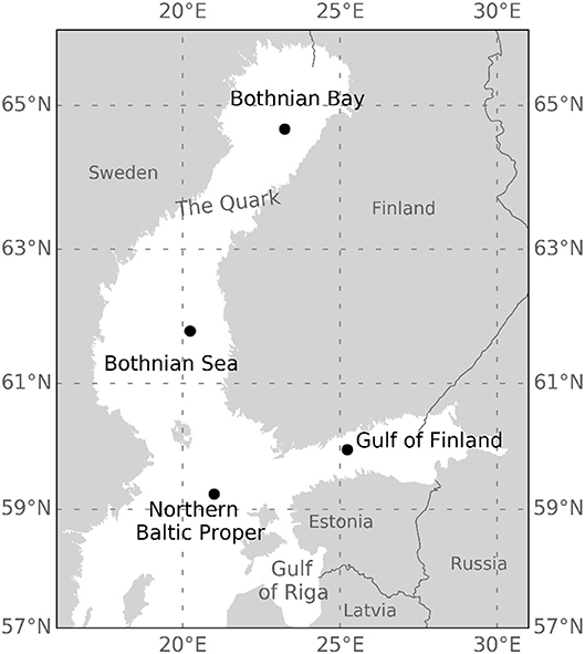
Figure 1. Sub-basins of the northern Baltic Sea and locations of the FMI wave buoys (black dots).
Third-generation wave models, such as WAM, WAVEWATCH III®, and SWAN, are able to account for ice conditions. Therefore, many of the existing wave hindcast statistics have somehow accounted for ice conditions (e.g., Günther et al., 1998; Swail et al., 2006; Reistad et al., 2011; Tuomi et al., 2011; Björkqvist et al., 2018). A typical way to account for ice in wave models is to exclude grid points from the calculations if the ice concentration is greater than a certain threshold value, e.g., 30% (Tuomi et al., 2011). A more sophisticated method to account for ice conditions has been presented by e.g., Tolman (2003), who proposed that ice concentration is treated as an additional grid obstruction, which attenuates the propagation of wave energy between the grid points. Recently, Doble and Bidlot (2013) also presented a method to attenuate the modeled wave energy in order to achieve better wave forecasts in the marginal ice zone. Furthermore, sophisticated source terms are being developed in order to account for wave-ice interaction in wave models more accurately (e.g., Rogers and Orzech, 2013; Rogers and Zieger, 2014; Rogers et al., 2016).
There are several different sources for ice data. In the Baltic Sea, one good source is the ice charts produced by the national Ice Services. The ice charts are based on combined information from satellite analyses, ice observations from ships and coastal measurement sites, and expert analyses. These products have existed in digitized format for at least the past 10–20 years. When making hindcasts for longer historical periods, or when making climate scenarios, ice concentrations produced by 3D ocean-ice models are typically used. The accuracy of the present state-of-the-art models in presenting the Baltic Sea ice conditions has been shown to be relatively good, e.g., by Löptien et al. (2013) and Pemberton et al. (2017). There are also satellite-based products such as OSISAF (Tonboe et al., 2016), which provide ice concentration data for northern and southern latitudes. However, their resolution is still quite coarse considering the small size and complex shape of the Baltic Sea.
In addition to the different sources of ice data—and the various ways to handle them—there is another complication in compiling wave statistics for seasonally ice-covered seas: how to handle the time of year when a sea area is ice covered and the significant wave height equals zero. A common approach is to include only values from the time when the sea is ice free (e.g., MacLaren Plansearch Limited, 1991). This is the prevailing method when measured data is presented. On the other hand, when wave statistics are used to estimate wave energy resources, the wave height is set to zero when there is ice (e.g., Cornett, 2008). The lack of historical sea ice data may also hinder the use of ice conditions when compiling wave statistics from model data (Gorman et al., 2003). Also, ignoring ice conditions in model calculations and in the formulation of statistics is the simplest way to compile wave hindcast statistics in seasonally ice-covered seas.
Tuomi et al. (2011) and Tuomi (2014) have presented five different ways to compile wave statistics in seasonally ice-covered sea areas. The statistics types are as follows: (1) measurement statistics (type M), (2) ice-time-included statistics (type I), (3) ice-free time statistics (type F), (4) hypothetical no-ice statistics (type N), and (5) exceedance time statistics (type ET). They differ in how they deal with the time when there is ice or when the data is missing. None of them is perfect, and each type has a specific application for which it is more suitable than the other types.
In this study, we use two different methods to handle the ice conditions in the wave model WAM. The first method excludes grid points from the calculations if the ice concentration exceeds a certain threshold value. This method was chosen since it has been traditionally used in operational forecasting and in wave hindcast statistics presented for the Baltic Sea. The second method is based on the work by Tolman (2003). This approach has been utilized in the Baltic Sea to account for unresolved coastal archipelagos (Tuomi et al., 2014) and also lately in the development of the CMEMS BAL MFC wave forecast (Tuomi et al., 2018). We also use ice information from two different sources: the daily ice concentrations from the Finnish Meteorological Institute's (FMI) ice service and daily mean ice concentrations from the Swedish Meteorological and Hydrological Institute's (SMHI) NEMO-Nordic simulation. The effect of the different handling of ice is studied by running the wave model for four different ice winters. The wave hindcasts are validated against altimeter measurements. Monthly mean, maximum, and exceedance statistics are presented for the northern Baltic Sea and differences between the four hindcasts in presenting the wave conditions and statistics are analyzed and discussed.
2. Modeling
We made simulations for four winters: 2009, 2010, 2011, and 2012. All simulations were run with the wave model WAM, using wind forcing from RCA4 down-scaled ERA-Interim. The simulations were run for January–April, which are the months that typically have an ice cover even in the mildest winters. We used two different methods to handle ice in the WAM model and two data sources for ice concentrations. The details of the modeling and forcing used are explained in the following Sections.
2.1. Wave Model WAM
We used the third-generation wave model WAM (WAMDI, 1988; Komen et al., 1994) to simulate the Baltic Sea wave field, which evolution is determined by calculating the wave energy spectrum. To this end, WAM solves the action balance equation, which in deep water without currents can be written for spherical coordinates as:
where F(t, ϕ, λ; θ, ω) is the spectral density, which is a function of the time t, the latitude ϕ and the longitude λ. The spectral density is also a function of the spectral variables describing the wave direction (θ) and the angular frequency (ω).
The velocities in the longitudinal and latitudinal directions are given by
where cg is the group velocity and R is the radius of the Earth. Finally, the change in wave direction in spectral space is given by
The left side of Equation (1) is solved numerically using a first-order upwind scheme.
The right side of Equation (1) lists the different sources and sinks that add, dissipate, or redistribute the energy in the wave spectrum. The deep-water source terms include the wind input (Sin, Janssen, 1991), the dissipation of waves due to whitecapping (Sds, Komen et al., 1994), and the discrete interaction approximation (DIA) of the nonlinear four-wave interactions (Snl, Hasselmann et al., 1985).
WAM has been developed to be used also in areas with finite depth (Monbaliu et al., 2000), and cycle 4.5.4, therefore also includes source terms to account for the bottom friction (Hasselmann et al., 1973) and the depth-induced wave breaking (Battjes and Janssen, 1978). In this study, all properties accounting for the finite depth were switched on.
We used a 1 nmi (c. 1.852 km) resolution grid for the Baltic Sea with additional grid obstructions for the coastal archipelagos in the northern Baltic Sea. The model wave spectra comprised of 36 directions and 35 frequencies (0.04177–1.06719 Hz). The same grid and model configuration is used in the CMEMS BAL MFC wave analysis and forecast system (marine.copernicus.eu, BALTICSEA_ANALYSIS_FORECAST_WAV_003_010), run by FMI (e.g., Tuomi et al., 2018).
2.2. Methods to Handle Ice in a Wave Model
A method to handle the seasonal ice cover has been present in FMI's operational wave model applications since 2001, when operational forecasts with a coupled atmosphere-wave model started (Järvenoja and Tuomi, 2002). At first, the ice conditions were handled by excluding grid points from the calculations if they had an ice concentration over 30%. Until 2009, this was done through a bathymetry modification by changing the ice-covered areas to land points. Since 2009, ice conditions have been handled by setting the energies in the wave spectrum to zero at points where the ice concentration exceeds the threshold value.
To further develop the methods to handle ice conditions in seasonally ice-covered seas, we used the method introduced by Tolman (2003) to treat unresolved ice in a wave model grid. We have previously implemented this method to account for the wave energy attenuation caused by unresolved islands in order to improve the quality of the WAM-model results in the coastal archipelagos of the northern Baltic Sea (Tuomi et al., 2014).
Tolman (2003) presented how the energy fluxes between the grid cells can be reduced according to subgrid-scale obstructions
where αi, − and αi, + are transparencies at cell boundaries and Gi, − and Gi, + are fluxes at the cell boundaries.
The transparencies at cell boundaries vary between 0 and 1, with 0 meaning a closed boundary and 1 a totally open boundary. The obstructions, land or ice, that are typically defined at the center of the grid boxes are converted to transparencies at cell boundaries according to
where αi is the obstruction at the cell center. The outflow transparency αi, + is set to 1 by default.
We used a threshold value of 70% to determine the treatment of the ice in a grid cell. When the ice concentration in a grid point was smaller than 70%, the ice was treated as additional grid obstruction, which reduced the energy between grid points according to Equation (5). Grid points having an ice concentration of over 70% were excluded from the calculations. Different wave model configurations are described in Table 1.
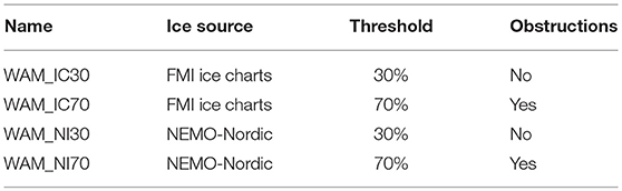
Table 1. WAM configurations.
The threshold values used for ice concentration in this study are based on the World Meteorological Organization (WMO) classification of ice compactness (WMO, 2015). In the classification, 30% is used as an upper limit for very open drift ice and 70% as a lower limit for close drift ice.
2.3. Forcing
2.3.1. Wind Forcing
We used downscaled ERA-Interim data (Dee et al., 2011) as a wind forcing for the wave model. The downscaling was done with the Swedish Meteorological and Hydrological Institute's regional climate model RCA4, using spectral nudging (Berg et al., 2013). The re-analysis is available for the years 1979–2013. The horizontal resolution of the forcing is 11 km, and the wind fields are available with 3-h intervals.
2.3.2. Gridded Ice Charts
FMI's Ice Service produces daily ice concentration maps, which are also available as a gridded product. The daily updated charts are compiled on the basis of satellite observations, available in-situ observation and expert analysis. For the period 2009–2012, the ice charts were available in gridded format with 0.02° × 0.01° resolution, for longitude and latitude, respectively. The ice concentrations were interpolated to the WAM grid points using the nearest neighbor method.
2.3.3. NEMO-Nordic
Daily mean ice concentrations from the SMHI NEMO-Nordic (e.g., Hordoir et al., 2019) simulation were used as forcing for the wave model. The data was available in 2 nmi (c. 3.7 km) resolution for the Baltic Sea region and the NEMO-Nordic simulations were run using the same atmospheric forcing as the WAM model runs (see description in section 2.3.1). The ice concentrations were interpolated to the WAM grid points using the nearest neighbor method.
3. Ice Winters 2009–2012
The winters 2009–2012 were selected for this study, since they included different types of Baltic Sea ice winters, namely one mild, one severe, and two average winters (Figure 2). The severity classification of the Baltic Sea ice season is based on the maximum extent of the ice cover from the winters 1960/1961 to 2009/2010. The severity of the winter is determined by the area of total extent compared to the long-term mean. A winter with a maximum extent below 115,000 km2 is classified as mild, while severe winters have a maximum extent of over 230,000 km2. The classification does not consider duration, ice concentration, thickness, or deformation degree.
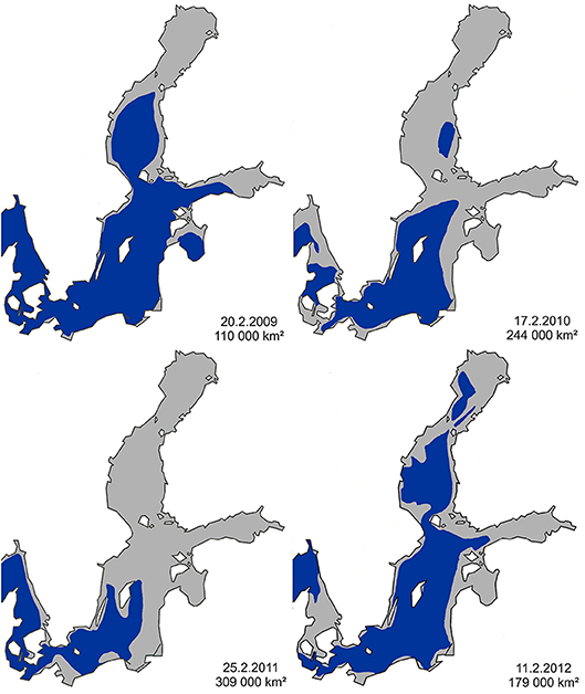
Figure 2. Maximum ice extent in the Baltic Sea in 2009 (Upper left), 2010 (Upper right), 2011 (Lower left), 2012 (Lower right). Open water is shown with blue color and ice-covered areas with gray.
The ice winter 2008/2009 was mild in the Baltic Sea, compared to the long-term average. There was a significant amount of sea ice only in the Bothnian Bay and the eastern part of the Gulf of Finland (Figure 2, upper left). In the Bothnian Bay, the freezing started after mid-November, which was 3 weeks later than the long-term average. Larger areas started to freeze in the beginning of January. The maximum ice extent occurred on February 20, which is 1 week earlier than an average winter. The Bothnian Sea and Gulf of Finland were mostly ice free by the April 19. By the end of May the Bothnian Bay was also free of ice, thus ending the ice season.
The ice winter of 2009/2010 was average when considering the maximum ice extent. However, the ice winter was over a month shorter than average in the northern parts of the Bothnian Bay. The ice season started in mid-December, and during January most of the Bothnian Bay was ice covered, along with coastal areas of the Bothnian Sea. The maximum ice extent was reached by February 17, almost 2 weeks earlier than on average (Figure 2, upper right). The Gulf of Finland and the Bothnian Sea were free of ice on April 19 and the Bothnian Bay on May 31.
Of the four winters in this study, the ice winter of 2010/2011 was the most severe. In the Bothnian Sea, the northern Baltic Proper, and the Gulf of Finland, the ice winter was between 2 and 6 weeks longer than the average. The maximum ice cover was reached on February 25 (Figure 2, lower left). By this time the Bothnian Bay, Bothnian Sea, Gulf of Finland, and Gulf of Riga, as well as the northern part of the Baltic Proper, were totally ice covered. At the end of February, southerly winds packed the ice toward the coast, thus reducing the ice-covered area while causing ice ridges and difficulties for the ship traffic. By May 14, the Gulf of Finland was completely ice-free, and 1 week later also the Bothnian Sea. The ice season ended on the May 24.
The ice winter of 2011/2012 was average based on the ice extent evaluation, but it started exceptionally late and also ended earlier than on average. In the Bothnian Bay the ice winter was from over 4 weeks to almost 6 weeks shorter than on average, and in the Bothnian Sea and the Gulf of Finland about 3 weeks shorter than on average. The northern Baltic Proper remained ice-free throughout the winter. The ice extent reached its maximum on February 11, 2 weeks earlier than on average (Figure 2, lower right). The Gulf of Finland was free of ice by the first week of May and the Bothnian Bay on May 19.
4. Validation
The validation of the wave model results in, and close to, the ice-covered areas is difficult. The wave buoys are usually recovered well before the sea area freezes, and in the northern part of the Baltic Sea the measurement period is typically from May/early June until December/early January.
We used altimeter data to get some estimate of how the two different ice products and two different ways to handle ice conditions in the wave model affected the quality of the wave hindcasts. Data were extracted from the IFREMER Global altimeter SWH data set (Queffeulou and Croizè-Fillon, 2017). For the period in question there were data from five different satellites, namely ERS2, ENVISAT, JASON1, JASON2, and CRYOSAT. We used corrected SWH values, which for ERS2, ENVISAT, JASON1 and JASON2 are based on Queffeulou (2004); Queffeulou et al. (2011), and for CRYOSAT on Queffeulou (2013). In the dataset, the ice covered areas have been masked out based on the Polar Sea Ice concentration product by CERSAT (cersat.ifremer.fr). In the Baltic Sea, Kudryavtseva and Soomere (2016) have evaluated, that ice starts to affect the altimeter SWH already with a 10% concentration and that the effects are notable at concentrations of 30%. Therefore, using the ice data to mask out the altimeter SWH values from partially ice-covered areas is important.
The comparison of the simulated and altimeter SWH was performed only for the Gulf of Bothnia, i.e., the Bothnian Sea, the Quark, and the Bothnian Bay. This area also has ice during mild winters, as described in section 3, and has been shown to have good-quality altimeter data when compared with wave buoy measurements (e.g., Kudryavtseva and Soomere, 2016).
The accuracy of the simulations was relatively good (Figure 3) and comparable to earlier wave model studies presented for this area (e.g., Tuomi et al., 2011). Generally, the lower values of SWH were underestimated and higher values (over 3.5 m) were overestimated by the model. The underestimation of the lower values of SWH was larger when the ice concentrations were obtained from NEMO-Nordic than for the runs using ice concentrations from the FMI ice charts. As the ice charts are based on satellite and in-situ data, this was expected. However, the differences were relatively small, indicating that the NEMO-Nordic can reproduce the ice concentrations quite well in the northern Baltic Sea. There were also some discrepancies resulting from the different ways to handle ice conditions, but these were significantly smaller than those arising from using different sources of ice data.
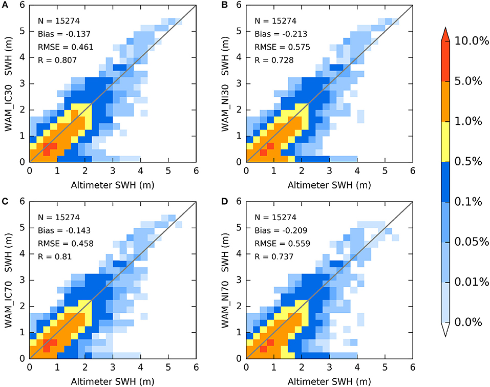
Figure 3. Scatter plots where the SWH from four model setups are compared to the altimeter SWH. The colors indicate the concentration of the values. Explanations of model setups (A) WAM_IC30, (B) WAM_NI30, (C) WAM_IC70, and (D) WAM_NI70 are presented in Table 1. Number of comparison points (N), bias, root-mean-square error (RMSE) and Pearson correlation (R) are presented together with each setup.
The comparison also revealed a few occasions when the altimeter measured a non-zero SWH, even though both ice data sources showed the grid cell to contain ice. There are fewer of these cases in the runs that use data from FMI's ice charts than in those using data from NEMO, and the discrepancy can mostly be attributed to small differences in the location of the ice edge between the different products.
Due to the small size and shape of the Baltic Sea, the accuracy of the modeled significant wave height is quite sensitive to the accuracy and resolution of the forcing wind field. The wind forcing used in this study (cf. section 2.3.1) has quite a coarse resolution, 11 km, and is intended for running hindcasts or reanalysis. We used it to have a consistent simulation with the NEMO-Nordic, which was run using the same meteorological forcing. The wave model setup used in this study, is also used in the CMEMS BAL MFC wave analysis and forecast system. Those forecasts utilize the operational FMI-HARMONIE wind fields with about 2.5 km horizontal resolution, which naturally leads to considerably better accuracy in simulated SWH (Tuomi et al., 2018; Vähä-Piikkiö et al., 2019).
5. Wave Statistics
The WAM simulations for Jan–Apr 2009–2012 were used to calculate the mean and maximum values of significant wave height. When presenting the statistics we use the ice-time-included statistics (type I, Tuomi et al., 2011), i.e., during the time when the sea area is ice-covered, the significant wave height is set to zero. These types of statistics give lower mean values in the seasonally ice-covered areas than the other statistics types. Considering the applications, for which type I statistics is a good choice, one example is the estimation of wave energy resources, as already discussed in Section 1. Recently, for example Nilsson et al. (2019), have used Type I statistics to evaluate the wave energy potential for the Baltic Sea. Type I statistics is also a good choice when evaluating the fatigue loads from waves on offshore structures, and similar phenomena of a cumulative nature in seasonally ice-covered seas, when the loads imposed by ice conditions are evaluated separately. Furthermore, type I statistics can be used when the wave-related requirements and economic risks for shipping are estimated for the lifetime of operations, which are carried out year-round.
5.1. Monthly Mean Values
The monthly mean values of SWH, calculated from the four wave model runs for 2009–2012, showed some differences (Figures 4, 5). The largest differences, up to 0.3 m, were between the runs using the ice chart (WAM_IC) and NEMO (WAM_NI) data. The different methods to handle ice resulted in considerably smaller differences, typically smaller than 0.05 m (Figures 4G,H). Therefore, for Feb–Apr, we only present the mean values of the WAM_IC30 and WAM_NI30 runs (Figure 5). The differences in the monthly mean SWH values between WAM_IC and WAM_NI resulted from the differences in the ice extent and the location of the ice edge in two ice products. In the Bothnian Bay, the use of NEMO-Nordic ice concentrations resulted in a lower mean SWH in every month. The choice of ice product also affected the values in the Quark and the Bothnian Sea. However, in these areas, the higher mean SWH was sometimes obtained when using NEMO-Nordic ice concentrations.
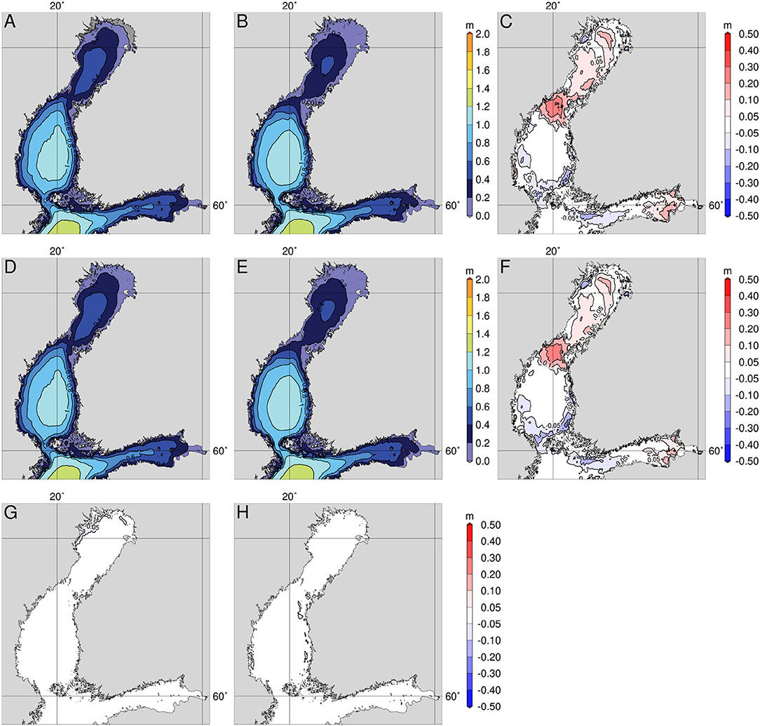
Figure 4. Mean values of significant wave height in January 2009–2012. Ice-included-time statistics, type I. (A) WAM_IC30. (B) WAM_NI30. (C) WAM_IC30–WAM_NI30. (D) WAM_IC70. (E) WAM_NI70. (F) WAM_IC70–WAM_NI70. (G) WAM_IC30–WAM_IC70. (H) WAM_NI30–WAM_NI70.
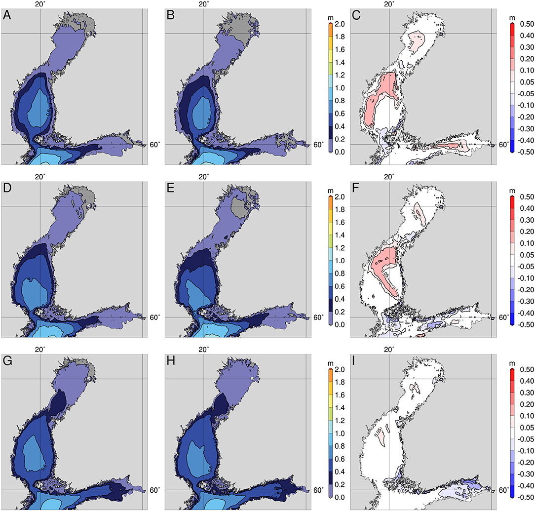
Figure 5. Mean values of significant wave height in February (A–B), March (D–E), and April (G–I) 2009–2012 for WAM_IC30 (A,D,G) and WAM_NI30 (B,E,H) and the difference between them (C,F,I; WAM_IC30–WAM_NI30).
The lower mean values of SWH when using the NEMO-Nordic ice concentration results from the overestimation of ice extent in the model reported e.g., by Pemberton et al. (2017). They also found that, on average, the ice cover increased faster and retreated earlier in NEMO-Nordic than in observations.
Of the individual years, the differences between WAM_IC and WAM_NI runs were largest in 2009 (not shown). During this year, the ice extent in NEMO-Nordic runs was considerably larger than in the FMI ice charts both in February and March. The ice winters of 2010 and 2011 had smaller differences, since almost the whole Gulf of Bothnian and Gulf of Finland was covered in ice during these times (cf. Figure 2). In 2012, there were differences mainly in the Bothnian Bay and the eastern part of the Gulf of Finland.
5.2. Monthly Maximum Values
There were larger differences between the monthly maximum values than the monthly mean values (Figures 6–9). The two ways to handle the ice conditions lead to the largest differences in the Bothnian Bay and in the northern part of the Bothnian Sea. In March, there were also differences in the northern Baltic Proper (Figure 8) caused by the ice concentrations below 30% in the FMI ice charts, which were treated as only partly open water in the WAM_IC70 run. The method by Tolman (2003) reduces the propagation of wave energy in partially ice-covered areas (cf. section 2.2), which leads to lower values of significant wave height. However, there were also some areas in which the runs utilizing the Tolman (2003) method gave higher maximum values than the runs using the 30% threshold value: for example, in February, in the northernmost part of Bothnian Bay and in the easternmost part of the Gulf of Finland (Figure 7). This will be further discussed in section 6.
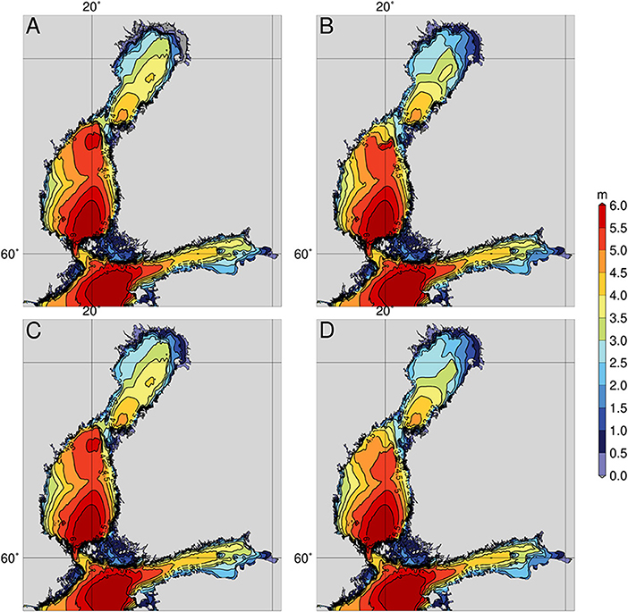
Figure 6. Maximum values of significant wave height in January 2009–2012 for (A) WAM_IC30, (B) WAM_NI30, (C) WAM_IC70, and (D) WAM_NI70.
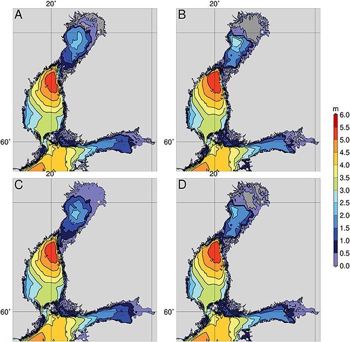
Figure 7. Maximum values of significant wave height in February 2009–2012 for (A) WAM_IC30, (B) WAM_NI30, (C) WAM_IC70, and (D) WAM_NI70.
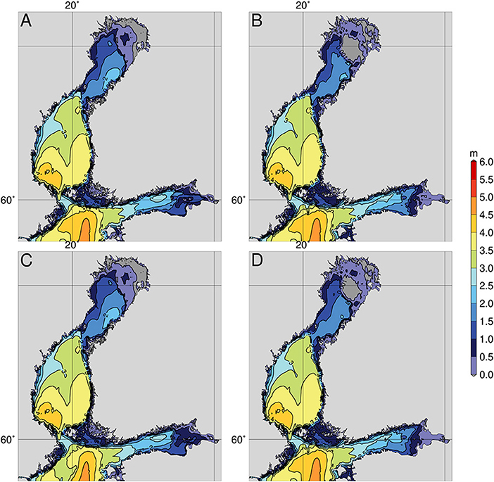
Figure 8. Maximum values of significant wave height in March 2009–2012 for (A) WAM_IC30, (B) WAM_NI30, (C) WAM_IC70, and (D) WAM_NI70.
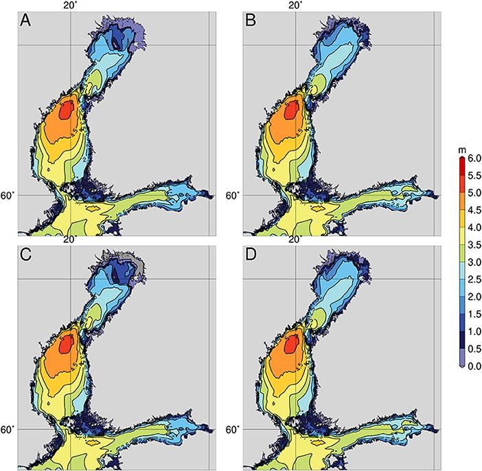
Figure 9. Maximum values of significant wave height in April 2009–2012 for (A) WAM_IC30, (B) WAM_NI30, (C) WAM_IC70, and (D) WAM_NI70.
There were also significant differences in the monthly maximum values between WAM_IC and WAM_NI. The largest differences were again in the Bothnian Bay, the northern part of the Bothnian Sea, and in the easternmost part of the Gulf of Finland. The largest difference was 3.2 m in January in the northern part of the Bothnian Sea near the Quark. The maximum value of SWH simulated by WAM_IC30 and WAM_IC70 was 5–6 m, whereas by WAM_NI30 and WAM_NI70, it was 2.5–4.5 m (Figure 6).
The situation resulting in the largest differences in the maximum values is shown in more detail in Figure 10. Although NEMO-Nordic simulates the ice extent fairly well, there was slightly more ice in the northern part of the Bothnian Sea than in the FMI ice charts. Because of this, WAM_NI30 and WAM_NI70 simulated no waves in the area where WAM_IC30 and WAM_IC70 produced the maximum values. This resulted in an over 5 m difference in the SWH in the northern part of the Bothnian Sea. The difference in the January maximum values is naturally lower, since there are other high wind situations in which the sea area has also been free from ice in the WAM_NI30 and WAM_NI70.
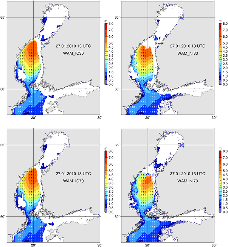
Figure 10. Wave hindcast for 27.1.2010 13 UTC with WAM_IC30 (Upper left), WAM_NI30 (Upper right), WAM_IC70 (Lower left), and WAM_NI70 (Lower right).
Figure 10 also shows how the additional grid obstructions affect the simulation of the wave field. The WAM_IC70 and WAM_NI70 runs showed slightly smaller values of significant wave height in the southwestern Bothnian Sea, north of the area, which was ice covered in all runs, than the WAM_IC30 and WAM_NI30 runs. All simulations showed the close drift ice field (ice concentration over 70%), but only the method relying on grid obstructions captured the surrounding, very open, drift ice field (ice concentration less than 30%). The grid obstruction attenuates the wave energy in the grid cells that have partial ice cover according to the method presented in section 2.2. The effect of the additional grid obstruction is demonstrated even better between the WAM_NI30 and WAM_NI70 runs in the north-western part of the Bothnian Sea, where WAM_NI70 produces lower values of SWH than WAM_NI30, since it is also able to account for ice concentrations less than 30%.
5.3. Statistics at Wave Buoy Locations
We studied the monthly statistics in more detail at four locations. The locations were selected to be those of FMI's operational wave buoy locations in the Bothnian Bay, the Bothnian Sea, the northern Baltic Proper, and the Gulf of Finland (locations shown in Figure 1). These sites represent open sea conditions for each of the sub-basins in the northern Baltic Sea.
The monthly mean, maximum and exceedance values at these locations showed that the differences between the four wave model simulations were relatively small in the Bothnian Sea (Figure 11) and in the Northern Baltic Proper (not shown). In the Gulf of Finland, the different sources of ice information had only small effects on the mean, maximum, and exceedance values when the 30% threshold value for ice concentration was used (Figure 11C). However, there were larger differences between the WAM_IC70 and WAM_NI70 runs, which used the grid obstructions (Figure 11F).
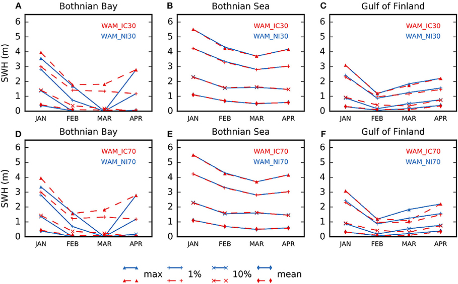
Figure 11. Monthly mean and maximum values of SWH and 1% and 10% exceedance values at 3 locations in the Baltic Sea (locations shown in Figure 1). (A,D) show statistics at the Bothnian Bay buoy location, (B,E) at the Bothnian Sea buoy location and (C,F) at the Gulf of Finland buoy locations. See Table 1 for further details about the model configurations.
In the Bothnian Bay, the differences between the simulations were larger than at the other locations (Figures 11A,D). The largest differences were in March, when WAM_IC30 and WAM_IC70 gave c. 1.8 m as the maximum value, whereas WAM_NI30 and WAM_NI70 gave 0 m. The maximum value from the WAM_IC30 and WAM_IC70 is from a high wind situation on March 16, 2012. The 2012 ice winter was average, but the length of the ice season was shorter than on average (cf. section 3). In mid-March the ice edge was close to the Bothnian Bay buoy location and retreated northward on 15–16th, which allowed higher waves to propagate into this location. In the simulations WAM_NI30 and WAM_NI70, the area is totally ice covered during March, leading to a maximum SWH of 0 m.
The histograms and cumulative probability distribution curves for the four buoy locations also show that the differences between WAM_IC30 and WAM_NI30 simulations are largest in the Bothnian Bay (Figure 12). In the Bothnian Sea and the northern Baltic Proper, the differences are small, almost nonexistent. The WAM_IC70 and WAM_NI70 differed only slightly from the WAM_IC30 and WAM_NI30, respectively and are, therefore, excluded from this analysis. The histograms also demonstrate that, in the Bothnian Bay and the Gulf of Finland, the ice season has the strongest effect on the wave climate. In the Bothnian Bay 83–88%, of the SWH values during Jan–Apr are in the range 0.00–0.25 m, while the corresponding percentages for the Gulf of Finland wave buoy location are 67–70%. In the Bothnian Sea buoy location, only 34% and in the Northern Baltic Proper, c. 12%.
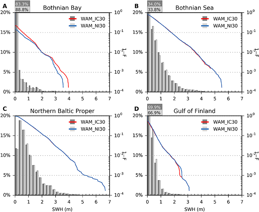
Figure 12. Histograms and cumulative probability distributions of hindcast SWH at the four wave buoy locations (A) Bothian Bay, (B) Bothian Sea, (C) Northern Baltic Proper and (D) Gulf of Finland (locations shown in Figure 1). Values for configuration WAM_IC30 are presented with dark gray and red and for WAM_NI30 with light gray and blue. The percentage of the first bin (0–0.25 m) is presented in the upper-left corner of the plot with corresponding color.
6. Wave Forecasting in Seasonally Ice-Covered Seas
Even though the different approaches to account for ice in the wave model induced only relatively small differences in the hindcast statistics, the effects can be considerably larger in operational wave forecasting. When using the method adapted from Tolman (2003), the threshold for a point to be completely excluded from the calculations is set to a relatively high value, such as 70%. Smaller ice concentrations are accounted for by additional grid obstruction, which allows for the forecasting of waves in areas that have only a partial ice cover, such as open drift ice fields. The grid obstructions also, at least to some extent, account for how the drift ice attenuates the waves.
To demonstrate what consequences the various ways to account for the ice conditions can have on the modeled wave field, we examined a high wind and wave situation from March 2011 in more detail. This occasion was discussed in section 5.2, since it caused large differences in the monthly maximum values in the northern Baltic Proper. The two approaches to implement the FMI ice chart data in the wave model produced different simulated significant wave heights in both the Bothnian Sea and in the northern Baltic Proper on March 9, 2011 at 18 UTC (Figure 13, upper panel). In the Bothnian Sea there was drift ice with a 40–60% concentration, which means that the 30% threshold completely excluded these points from the calculations. Still, the significant wave height in these areas was 0.5–1 m when the 70% threshold and additional grid obstructions were used. Conversely, in the northern Baltic Proper north off the Gotland island, there was a drift ice field with a concentration of only 10–30%. With the 30% threshold value, these grid points were considered as completely open water, while the grid obstructions captured the effect of the drift ice on the growth and propagation of the waves, thus leading to considerably lower wave heights (Figure 13, upper panel).
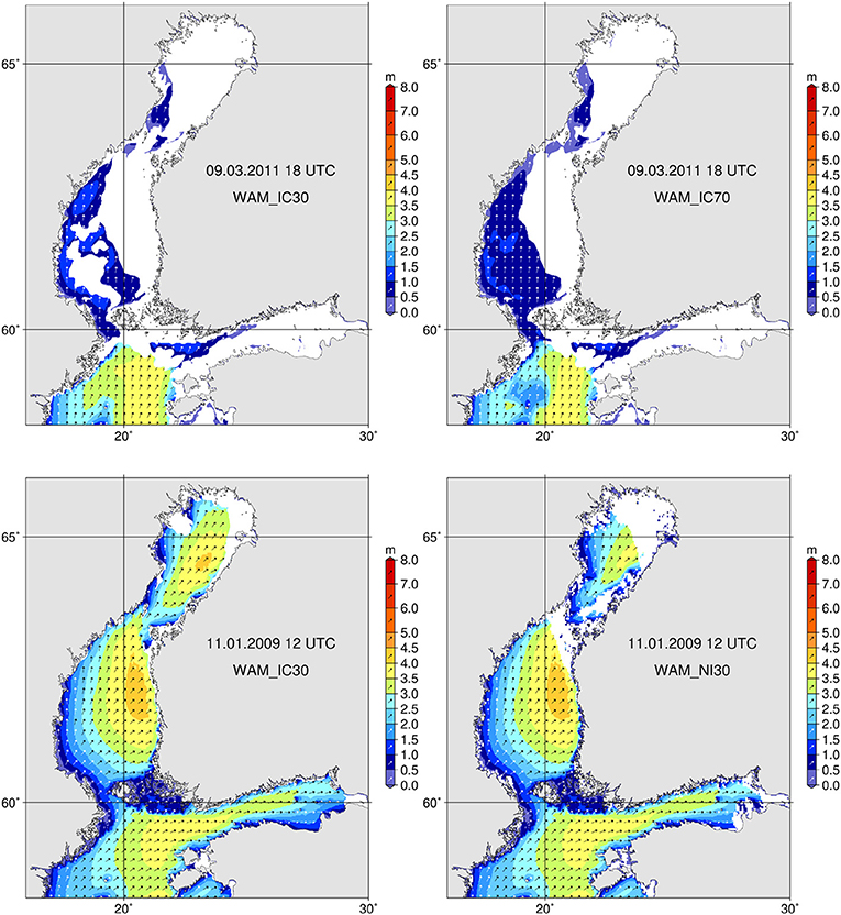
Figure 13. Wave hindcast for 9.3.2011 18 UTC with WAM_IC30 (Upper left) and WAM_IC70 (Upper right) and for 11.1.2009 12 UTC with WAM_IC30 (Lower left) and WAM_NI30 (Lower right).
As discussed earlier, the ice conditions shorten the fetch over which the waves grow, while also changing the fetch geometry. On Jan 11, 2009, there was a high wind situation in the Gulf of Bothnia inducing over 3 m significant wave heights both in the Bothnian Sea and in the Bothnian Bay (Figure 13, lower left panel). During this occasion, the NEMO-Nordic simulated ice in the Quark and in the eastern part of the Bothnian Bay, although no ice was present in the FMI ice charts. The NEMO-ice completely changed the fetch conditions in the Bothnian Bay, leading to lower significant wave heights (Figure 13, lower right panel). These types of differences in the ice concentrations can also have quite a significant impact on the exceedance values and maximum values of the significant wave height, as already shown in section 5.3. Nevertheless, the differences would most likely be minimized if a longer hindcast period was used.
7. Discussion
We presented two different methods to handle ice conditions in wave model simulations and ran the wave model WAM using two different sources for ice concentrations, namely FMI ice charts and an SMHI NEMO-Nordic hindcast. The results showed that, in most of the areas, the choice of data source had a larger impact on the results than the choice of the method with which the ice concentrations were handled in the wave model. This is quite expected, since the two ways to handle ice only result in small differences in the wave field, typically near the ice edge.
We did not evaluate the accuracy of the ice concentrations used in this study. The ice concentrations simulated by NEMO-Nordic have been evaluated in Pemberton et al. (2017). They found, that, overall the NEMO-Nordic simulated ice concentrations with relatively good accuracy, but the ice extent was slightly overestimated in the Gulf of Bothnia, and the ice winter started and ended earlier compared to the observations. The FMI ice charts or ice charts produced by the other operational centers in the Baltic are the best available information of the Baltic Sea ice conditions, as they are based on satellite data, in-situ measurements, and expert evaluations. Also, the validation against altimeter data showed that the WAM runs, using FMI ice chart data, were more accurate than those forced with NEMO-Nordic ice concentrations. The differences in the monthly mean values, however, were relatively small and mostly related to the slightly larger ice extent in the NEMO-Nordic hindcasts compared to the FMI ice charts. This resulted in somewhat smaller values of mean SWH for model runs forced with NEMO ice, especially in the Bothnian Bay and in the Gulf of Finland. The monthly maximum values showed larger differences, up to 3.2 m in the northernmost part of the Bothnian Sea, and there were also significant differences in other areas. For example, the more detailed analysis of the wave statistics at the buoy locations showed that, in the Bothnian Bay, the four simulations lead to considerable differences in the maximum and 1% exceedance values. The analysis of the maximum values for the northern Baltic Sea indicated that similar differences between the WAM_IC and WAM_NI runs also exist in the Quark area and in the coastal areas of the Bothnian Sea.
Because the Baltic Sea is small, the changes in fetch are important for the generation of waves. The location of the ice edge, therefore, becomes an important factor in the high-wind and storm situations, as demonstrated in section 5.2 (Figure 10) and section 6 (Figure 13, lower panel). We also showed that, under such weather conditions the use of obstruction grids might become important, since they can capture the attenuating effect of possible drift ice fields that have a relatively low ice concentration. However, it is difficult to evaluate, the accuracy of the wave simulations near the ice edge or in the drift ice field, since there are no measurements to compare the results against. To further develop the wave modeling during the Baltic Sea ice winter, measurements with instruments that are able to measure waves in the ice field and near the ice edge are needed.
In this study, we only modeled the months that have significant ice cover in the Baltic Sea, namely Jan–Apr. Therefore, only the differences in the monthly statistics could be studied. Most of the earlier studies in the Baltic Sea handle either annual or seasonal statistics. We estimate that the differences in the annual wave statistics will be smaller than the ones presented here for the monthly statistics, since the ice season only covers less than 6 months of the year and outside ice season, the different methods results to exactly the same SWH. In seasonal statistics, the differences can be significant, for winter and spring seasons, at least in the Bothnian Bay and the Gulf of Finland. However, 4 years is a relatively short time to study maximum values, especially in monthly stratified statistics. The differences will most likely diminish when longer periods are used.
The temporal resolution of the ice data used in this study was 1 day. In operational forecasting, when the ice is taken from a 3D ocean-ice model, such as NEMO-LIM3, the ice fields could be updated hourly. This means that the changes in the ice conditions during the forecast run can be accounted for with higher temporal resolution, leading to better estimates of the SWH, especially in high-wind and storm situations, when there can be quite rapid changes in the ice concentration.
The data and methods used in this study only included ice concentrations. Other parameters, such as ice thickness, can be important in the wave–ice interactions. For example, thin new ice is more easily broken and fragmented by waves than, for example, thick landfast ice. However, accounting for these types of interactions, a coupled wave–ice model is needed.
8. Conclusions
We made a wave hindcast study to illustrate how different methods to handle ice conditions in the wave model simulations and different sources for ice data affect the wave model results, wave hindcast statistics, and operational wave forecasts.
The comparison against altimeter data showed that the accuracy of the wave hindcasts during the ice season was better, when FMI ice charts were used as the source of ice concentrations compared to the runs where ice concentrations were taken from SMHI NEMO-Nordic simulations.
There were only small differences in the monthly mean values of SWH between the four runs. The differences were up to 0.3 m and were seen in the Bothnian Bay, the Quark, the northern part of the Bothnian Sea, and the eastern part of the Gulf of Finland. In the Bothnian Bay, the use of NEMO ice data lead to smaller mean values for all the months (Jan–Apr) studied in this paper. In other areas, the mean values produced by runs using NEMO ice data could also be higher than those using data from FMI ice charts. In the maximum values, the differences were larger, up to 3.2 m, since in individual high-wind or storm situations, the location of ice edge and the existence and location of drift ice fields becomes important. Also, in the exceedance values studied at the buoy locations, representing the open sea conditions in each of the northern Baltic Sea sub-basins, there were significant differences in the Bothnian Bay and in the Gulf of Finland. In the Bothnian Sea and Northern Baltic Proper buoy locations, the differences between the four hindcast runs were insignificant.
The ice charts were naturally found to be a better source for ice data in the Baltic Sea wave hindcasts than the NEMO-Nordic ice concentrations. However, the differences were quite small in the mean values and when running wave hindcasts for periods for which ice charts data are not available in digitized form, using data from 3D ocean–ice model leads to sufficient accuracy in most of the Baltic Sea sub-basins. Furthermore, ice concentration forecasts provided by a 3D ocean-ice model, might improve the wave forecasts accuracy in high wind situations, when there can be large changes in the ice field.
The use of the two different methods to handle ice concentrations in the wave model resulted only in small differences in the monthly statistics. However, in specific situations the two methods lead to significant differences in the hindcast wave field. Although, it was not possible to verify the accuracy of the wave hindcasts in areas and times these differences occurred, the possibility to provide wave forecast to partially ice-covered areas supports the use of handling ice as additional grid obstructions in operational wave forecasting.
Author Contributions
LT had the original idea for this research work, and she performed the WAM simulations and most of the data analysis. HK was responsible for the model validation and formulating and analyzing the statistics at the buoy locations. HK and J-VB contributed to the analysis of the wave statistics. RH and AH performed the NEMO runs, from which the ice concentrations were used in the wave model simulations. RM developed the programs for analyzing the monthly mean and maximum statistics. JV analyzed the FMI ice chart data. KK enlightened the ways different types of statistics can be applied. LT and HK wrote the paper with help from all the co-authors.
Funding
This work has been supported by the Strategic Research Council at the Academy of Finland, project SmartSea (grant number 292 985) and E.U. Copernicus Marine Service Programme.
Conflict of Interest Statement
RM was employed by the Finnish Meteorological Institute at the time of the study, but has since moved to Eniram Ltd. This has no impact on the research conducted.
The remaining authors declare that the research was conducted in the absence of any commercial or financial relationships that could be construed as a potential conflict of interest.
Acknowledgments
We thank SMHI for making the wind forcing from SMHI-RCA4 down-scaled ERA Interim available to us. Altimeter SWH data was extracted from the merged altimeter dataset produced by IFREMER.
References
Battjes, J. A., and Janssen, J. P. F. M. (1978). “Energy loss and set-up due to breaking of random waves,” in Proceedings of the 16th International Conference on Coastal Engineering (New York, NY: American Society of Civil Engineers), 569–587.
Berg, P., Döscher, R., and Koenigk, T. (2013). Impacts of using spectral nudging on regional climate model RCA4 simulations of the Arctic. Geosci. Model Dev. 6, 849–859. doi: 10.5194/gmd-6-849-2013
Björkqvist, J.-V., Lukas, I., Alari, V., van Vledder, G. P., Hulst, S., Pettersson, H., et al. (2018). Comparing a 41-year model hindcast with decades of wave measurements from the Baltic Sea. Ocean Eng. 152, 57–71. doi: 10.1016/j.oceaneng.2018.01.048
Cornett, A. (2008). “A global wave energy resource assesment,” in Proceedings of the Eighteenth (2008) International Offshore and Polar Engineering Conference (Vancouver, BC), 318–326.
Dee, D. P., Uppala, S. M., Simmons, A. J., Berrisford, P., Poli, P., Kobayashi, S., et al. (2011). The ERA-Interim reanalysis: configuration and performance of the data assimilation system. Q. J. R. Meteorol. Soc. 137, 553–597. doi: 10.1002/qj.828
Doble, M. J., and Bidlot, J.-R. (2013). Wave buoy measurements at the Antarctic sea ice edge compared with an enhanced ECMWF WAM: Progress towards global waves-in-ice modelling. Ocean Model. 70, 166–173. doi: 10.1016/j.ocemod.2013.05.012
Gorman, R. M., Bryan, K. B., and Laing, A. K. (2003). Wave hindcast for the New Zeland region: deep-water wave climate. N. Z. J. Mar. Freshw. Res. 37, 589–612. doi: 10.1080/00288330.2003.9517191
Günther, H., Rosenthal, W., Stawarz, M., Carretero, J., Gomez, M., Lozano, I., et al. (1998). The wave climate of the Northeast Atlantic over the period 1955-1994: the WASA wave hindcast. Glob. Atmos Ocean Syst. 6, 121–163.
Hasselmann, K., Barnett, T. P., Bouws, E., Carlson, H., Cartwright, D. E., Enke, K., et al. (1973). Measurements of wind-wave growth and swell decay during the Joint North Sea Wave Project (JONSWAP). Dtsch. Hydrogr. Zeitschrift 12, 1–95.
Hasselmann, S., Hasselmann, K., Allender, J. H., and Barnett, T. P. (1985). Computations and parameterizations of the nonlinear energy transfer in a gravity-wave spectrum. Part II: Parameterizations of the nonlinear energy transfer for application in wave models. J. Phys. Oceanogr. 15, 1378–1391.
Hordoir, R., Axell, L., Höglund, A., Dieterich, C., Fransner, F., Gröger, M., et al. (2019). Nemo-Nordic 1.0: a NEMO-based ocean model for the Baltic and North seas-research and operational applications. Geosci. Model. Dev. 12, 363–386. doi: 10.5194/gmd-12-363-2019
Janssen, P. A. E. M. (1991). Quasi-linear theory of wind-wave generation applied to wave forecasting. J. Phys. Oceanogr. 21, 1631–1642.
Järvenoja, S., and Tuomi, L. (2002). Coupled atmosphere-wave model for FMI and FIMR. Hirlam Newslett. 40, 9–22.
Komen, G. J., Cavaleri, L., Donelan, M., Hasselmann, K., Hasselmann, S., and Janssen, P. A. E. M. (1994). Dynamics and Modelling of Ocean Waves. Cambridge: Cambridge University Press.
Kudryavtseva, N. A., and Soomere, T. (2016). Validation of the multi-mission altimeter wave height data for the Baltic Sea region. Estonian J. Earth Sci. 65, 161–175. doi: 10.3176/earth.2016.13
Löptien, U., Mårtensson, S., Meier, H. E. M., and Höglund, A. (2013). Long-term characteristics of simulated ice deformation in the Baltic Sea (1962-2007). J. Geophys. Res. 118, 801–815. doi: 10.1002/jgrc.20089
MacLaren Plansearch Limited (1991). Wind and Wave Climate Atlas Volume I, The East Coast of Canada. Transport Canada Publication No. TP10820E.
Monbaliu, J., Padilla-Hernández, R., Hargreaves, J. C., Albiach, J. C. C., Luo, W., Sclavo, M., et al. (2000). The spectral wave model, WAM, adapted for applications with high spatial resolution. Coast. Eng. 41, 41–62. doi: 10.1016/S0378-3839(00)00026-0
Nilsson, E., Rutgersson, A., Dingwell, A., Björkqvist, J.-V., Pettersson, H., Axell, L., et al. (2019). Characterization of wave energy potential for the Baltic Sea with focus on the Swedish Exclusive Economic Zone. Energies 12:793. doi: 10.3390/en12050793
Pemberton, P., Löptien, U., Hordoir, R., Höglund, A., Schimanke, S., Axell, L., et al. (2017). Sea-ice evaluation of NEMO-Nordic 1.0: a NEMO–LIM3.6-based ocean–sea-ice model setup for the North Sea and Baltic Sea. Geosci. Mod. Dev. 10, 3105–3123. doi: 10.5194/gmd-10-3105-2017
Queffeulou, P. (2004). Long term validation of wave height measurements from altimeters. Mar. Geodesy 27, 495–510. doi: 10.1080/01490410490883478
Queffeulou, P., Ardhuin, F., and Lefèvre, J.-M. (2011). “Wave height measurements from altimeters: validation status and applications,” in OSTST Meeting, 19–21 October, 2011 (San Diego, CA).
Queffeulou, P., and Croizè-Fillon, D. (2017). Global Altimeter SWH Data Set. Technical report, Laboratoire d'Océanographie Physique et Spatiale, IFREMER, Plouzané.
Reistad, M., Breivik, Ø., Haakenstad, H., Aarnes, O. J., Furevik, B. R., and Bidlot, J.-R. (2011). A high-resolution hindcast of wind and waves for the North Sea, the Norwegian Sea, and the Barents Sea. J. Geophys. Res. 116:C05019. doi: 10.1029/2010JC006402
Rogers, W., and Orzech, M. D. (2013). Implementation and Testing of Ice and mud Source Functions in Wavewatch III.® NRL Memo. Rep. NRL/MR/7320-13-9462, Naval Research Laboratory, Washington, DC.
Rogers, W., and Zieger, S. (2014). “New wave-ice interaction physics in WAVEWATCH III®,” in Proceedings of 22nd IAHR International Symposium on Ice (Singapore: International Association for Hydro-environment Engineering and Research (IAHR)).
Rogers, W. E., Thomson, J., Shen, H. H., Doble, M. J., Wadhams, P., and Cheng, S. (2016). Dissipation of wind waves by pancake and frazil ice in the autumn Beaufort Sea. J. Geophys. Res. 121, 7991–8007. doi: 10.1002/2016JC012251
Squire, V. A. (2018). A fresh look at how ocean waves and sea ice interact. Philos. Trans. R. Soc. Lond. A Math. Phys. Eng. Sci. 376:2129. doi: 10.1098/rsta.2017.0342
Squire, V. A., Dugan, J. P., Wadhams, P., Rottier, P. J., and Liu, A. K. (1995). Of ocean waves and sea ice. Annu. Rev. Fluid Mech. 27, 115–168. doi: 10.1146/annurev.fl.27.010195.000555
Swail, V., Cardone, V., Ferguson, M., Gummer, D., Harris, E., Orelup, E., et al. (2006). “The MSC50 wind and wave reanalysis,” in 9th International Wind and Wave Workshop, September 25–29 (Victoria, BC).
Tolman, H. L. (2003). Treatment of unresolved islands and ice in wind wave models. Ocean Model. 5, 219–231. doi: 10.1016/S1463-5003(02)00040-9
Tonboe, R., Lavelle, J., Pfeiffer, R.-H., and Howe, E. (2016). Product User Manual for OSI SAF Global Sea Ice Concentration. Technical report. Product OSI-401-b, Version 1.4.
Tuomi, L. (2014). On modelling waves and surface mixing in the Baltic Sea (Ph.D. thesis). Finnish Meteorological Institute - Contributions, No. 104. Helsinki, Finland.
Tuomi, L., Kahma, K. K., and Pettersson, H. (2011). Wave hindcast statistics in the seasonally ice-covered Baltic Sea. Boreal Environ. Res. 16, 451–472.
Tuomi, L., Pettersson, H., Fortelius, C., Tikka, K., Björkqvist, J.-V., and Kahma, K. K. (2014). Wave modelling in archipelagos. Coast. Eng. 83, 205–220. doi: 10.1016/j.coastaleng.2013.10.011
Tuomi, L., Vähä-Piikkiö, O., Siili, T., and Alari, V. (2018). “CMEMS Baltic Monitoring and Forecasting Centre: high-resolution wave forecasts in the seasonally ice-covered Baltic Sea,” in Operational Oceanography serving Sustainable Marine Development. Proceedings of the Eight EuroGOOS International Conference. 3-5 October 2017, Bergen, Norway, eds E. Buch, V. Fernàndez, D. Eparkhina, P. Gorringe, and G. Nolan (Brussels: EuroGOOS).
Vähä-Piikkiö, O., Tuomi, L., and Huess, V. (2019). Quality Information Document (QUID) Baltic Sea Wave Analysis and Forecasting Product BALTICSEA_ANALYSIS_FORECAST_WAV_003_010: issue 2.0. Technical report.
Keywords: wave modeling, seasonal ice cover, forecasting, statistics, Baltic Sea
Citation: Tuomi L, Kanarik H, Björkqvist J-V, Marjamaa R, Vainio J, Hordoir R, Höglund A and Kahma KK (2019) Impact of Ice Data Quality and Treatment on Wave Hindcast Statistics in Seasonally Ice-Covered Seas. Front. Earth Sci. 7:166. doi: 10.3389/feart.2019.00166
Received: 04 December 2018; Accepted: 14 June 2019;
Published: 10 July 2019.
Edited by:
Martin Stendel, Danish Meteorological Institute (DMI), DenmarkReviewed by:
Tarmo Soomere, Tallinn University of Technology, EstoniaXander Wang, University of Prince Edward Island, Canada
Copyright © 2019 Tuomi, Kanarik, Björkqvist, Marjamaa, Vainio, Hordoir, Höglund and Kahma. This is an open-access article distributed under the terms of the Creative Commons Attribution License (CC BY). The use, distribution or reproduction in other forums is permitted, provided the original author(s) and the copyright owner(s) are credited and that the original publication in this journal is cited, in accordance with accepted academic practice. No use, distribution or reproduction is permitted which does not comply with these terms.
*Correspondence: Laura Tuomi, bGF1cmEudHVvbWlAZm1pLmZp