Nighttime Cooling of an Urban Pond

One of the processes by which open water cools the air during hot summer days is by storing the heat and increasing its own temperature. This heat is then released at night. The aim of this paper is to analyze this cooling process by quantifying the magnitude of turbulent, latent and sensible, heat fluxes in comparison to radiative and ground fluxes. A detailed vertical temperature profile was measured in an urban pond (~70 cm deep with surface area of 3,627 m²) in Delft (NL) using Distributed Temperature Sensing for a period of one month. The results show that, from the total of 2.7 MJm⁻² of heat released by the pond on an average summer night, 43% of the thermal energy is emitted as longwave radiation, 39% as latent energy, and only 11% as sensible heat. An additional 0.10–0.32 MJm⁻² is transferred into the bottom of the lake. Temperature distribution and cooling of the water profile is influenced by weather conditions during the preceding day. This paper provides an insight into a behavioral pattern of an urban pond at night. The results can shed some light into the potential of urban bodies to increase the air temperature of their surroundings at night.

1. Introduction

High air temperatures can have a negative effect on human health and well-being. Several studies have shown that higher temperatures can lower the quality of sleep, and increase the risk of respiratory illnesses and cardiovascular mortality (e.g., Patz et al., 2005; Tan et al., 2007). Impact of extreme heat on humans is especially visible in cities, because urban areas generally experience higher temperatures than rural areas. Such Urban Heat Islands (UHI) are mostly caused by different heat capacities and albedo of urban surfaces, lower evaporation, anthropogenic heat production, and the specific geometry of street canyons (Oke et al., 1991; Lee, 1993; Ryu and Baik, 2012; Gago et al., 2013).

One of the possible ways to decrease air temperature in the urban environment is to increase evaporation by open water, such as ponds, channels, or fountains. Comparative studies have shown that from all the urban land use types, open water is the most efficient in reducing UHI at a local scale (e.g., Rinner and Hussain, 2011; Olah, 2012). Already a small pond can reduce temperature in its surroundings up to several degrees (Halper et al., 2012), especially in the morning, when the evaporative cooling effect is the strongest (Hathway and Sharples, 2012). Most pronounced influence of open water on temperature was measured close to the shore (Xu et al., 2010) and an effect of a big enough lake can be observed even at several kilometers (Theeuwes et al., 2013). Several studies agreed that proximity to open water dampens the diurnal temperature pattern (e.g., Wang et al., 2011; Theeuwes et al., 2013; CPC-Consortium, 2014; Steeneveld et al., 2014).

Strongest UHI is generally measured at night (Oke, 1982). Although the absolute temperatures are lower at night, the differences between urban and rural temperatures are at its maximum. In contrast to their daytime cooling effect, urban water bodies might contribute to higher air temperatures at night(Albers et al., 2015). Water has a high thermal inertia, which causes water bodies to have relatively high temperature at the end of a night compared to other urban land use types (Oswald et al., 2012; Yang and Zhao, 2015). Nonetheless, some studies concluded that water bodies provide cooling effect also at night, although to a limited extent (Coutts et al., 2012; Syafii et al., 2016).

The way urban water bodies influence air temperature at night has not been extensively studied so far and reported measurements show contradictory results. A comprehensive literature review by Manteghi et al. (2015) identified a lack of research about the potential night-time heating effect of urban water bodies, and a need for understanding the mechanisms.

This research aims to contribute to the understanding of thermal behavior of an urban pond during summer nights. This paper provides an analysis of temperature measurements and meteorological data from an urban pond in Delft, The Netherlands. We quantify the energy balance over the night, hence the magnitude of turbulent, sensible and latent, heat fluxes in comparison to radiative and ground fluxes, and the total decrease in temperature of the water.

2. Methods

2.1. Measurement Location

The measurements took place from 12 July till 7 August, 2014 in a shallow urban pond in Delft, The Netherlands (52.007° N, 4.375° E). The climate of The Netherlands is a moderate oceanic climate with summer starting in June and ending mid-late September. We chose a representative urban setting with an office building to the north and a residential building to the south. Several family houses with small gardens were located in the north-western direction from the setup and to the east was a quiet street with four floor residential buildings. The water was highly turbid and stagnant, except for rain conditions when the runoff from the streets was redirected to the pond. Water depth was ~70 cm and the average area of water surface is 3,627 m². The bed of the pond was covered with a soft layer of decomposing leaves. The pond had grassy embankments.

A vertical temperature profile was measured in the pond using Distributed Temperature Sensing (DTS). DTS is based on the backscatter of a laser beam traveling through a fiber optic cable and can be used for high-resolution temperature measurements. More information about this method can be found in Selker et al. (2006) and Tyler et al. (2009).

A downside of DTS is that during daytime, this method can lead to inaccuracies in temperature measurements due to incoming solar radiation (Hilgersom et al., 2016). For nighttime measurements, this is not a problem. Additionally, the measurement setup was shaded during the early morning hours and late evening. The late-evening shading ensured that the construction was not heated by the incoming solar radiation after sunset (Hilgersom et al., 2016).

Two DTS setups were placed in the north-east corner of the pond, each in the form of a 200 cm long transparent PVC tube with a diameter of 11 cm. To ensure ventilation, four 2 cm diameter holes were drilled every 6–8 cm in the tube. An optical cable was wrapped around the perforated tube with 0.50 cm spacing (see Figure 1). Temperature was measured every 5 min using a Silixa Ultima (Silixa Ltd., Hertfordshire, UK) with 0.126 m sampling resolution. Resulting measured vertical resolution of the described set-up was 0.18 cm. One column (right one in Figures 1a,b) was used for the analysis. The other column was used to study potential spatial differences in the pond. Temperature differences between the two measurement columns can be found in Supplementary Material. All data can be accessed at 4TU repository (Solcerova et al., 2017).

FIGURE 1

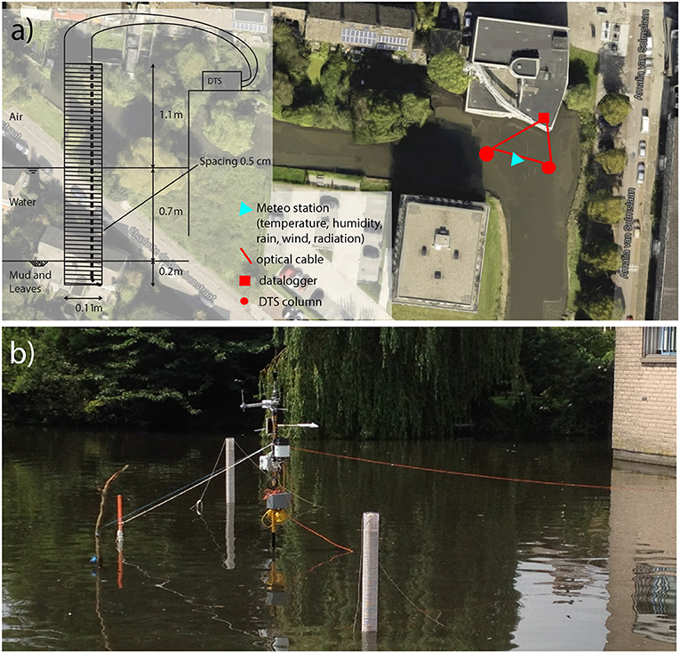
Figure 1. (a) Positioning of measurements in an urban pond in Delft, and detailed scheme of the DTS measurement setup. (b) View of the setup from the western shore of the pond. Water depth is about 0.7 m, the columns reached about 0.2 cm into the mud and leaves layer at the bottom of the pond.

A fully equipped HOBO weather station (Onset Computer CO., Bourne, MA, USA) was placed in between the two DTS columns. A full set of atmospheric variables was monitored during the whole experiment including atmospheric pressure, air temperature, relative humidity, wind speed and wind direction, and precipitation. Additionally, incoming and outgoing short- and long-wave radiation was measured using a CNR4 radiometer (Kipp & Zonen, The Netherlands).

2.2. Analysis Methodology

The analysis focuses only on the night-time. Night-time was defined as the time when incoming shortwave radiation equalled zero for all the days of the measurement period. After adjusting for different sunset and sunrise times the night was defined as the period between 23:00 and 5:00 CEST.

Conditions above an urban pond at night are predominantly unstable; the water is warmer than the air. On top of that, during our experiment the wind speeds were very low, on average 1.0 ms⁻¹. Due to these circumstances the standard calculation of sensible and latent heat flux using bulk aerodynamic method (Hicks, 1975) was not possible. The wide scale of measured meteorological variables and a detailed temperature profile allowed us to calculate the Bowen ratio [B [−], Bowen, 1926; Barr et al., 1994] and subsequently derive the turbulent fluxes.

$\begin{array}{ll}B=\frac{H}{E}& (\mathrm{1a})\end{array}$

$\begin{array}{ll}B=\frac{C_p(T_{ws}-T_a)}{\lambda (q_s-q_z)}& (\mathrm{1b})\end{array}$

where H [Wm⁻²] is the sensible heat, E [Wm⁻²] is the latent heat, C_p = 1006.43 J kg⁻¹K⁻¹ is the specific heat of air, λ is the latent heat of evaporation of water [J kg⁻¹], T_a is air temperature [°C], T_ws is water surface temperature [°C], q_s is saturated specific humidity at water-surface temperature [kg kg⁻¹], and q_z is specific humidity [kg kg⁻¹]. λ, q_s, and q_z were calculated for each time step (Abbasi et al., 2017).

$\begin{array}{ll}\lambda =2.501*10^6-2361T_a& (2)\end{array}$

$\begin{array}{ll}{q}_s=\frac{0.6108e_{sat}}{P_{atm}}& (3)\end{array}$

$\begin{array}{ll}{q}_z=\frac{0.6108e_a}{P_{atm}}& (4)\end{array}$

where e_sat [kPa] is saturated vapor pressure, e_a [kPa] actual vapor pressure, and P_atm [kPa] is atmospheric pressure. e_sat and e_a were calculated using Tetens equation.

Additionally, water surface temperature was calculated from measured outgoing longwave radiation using Stefan-Boltzmann law. Although it would be potentially possible to use DTS setup, surface temperature as measured by DTS is subject to complex small scale convective processes (Solcerova et al., 2018). For this reason, surface temperature as measured by outgoing longwave radiation, which integrates over a large area, is seen as more robust and is used throughout this paper.

$\begin{array}{ll}{T}_{ws}=\sqrt[4]{\frac{R{l}_{out}}{\sigma ϵ}}& (5)\end{array}$

where T_ws the surface temperature [K], Rl_out is the measured outgoing longwave radiation [Wm⁻²], ϵ = 0.98 [–] the emissivity of water (Wen-Yao et al., 1987), and σ = 5.67^*10⁻⁸ Wm⁻²K⁻⁴ the Stefan-Boltzmann constant.

Some of the measured outgoing longwave radiation will be incoming longwave reflected by the water surface, which has an albedo of (1-ϵ). It is difficult to come to an accurate estimate of this part of the radiative balance because the surrounding buildings make for a geometrically complex surrounding. Typical night-time values of outgoing and incoming longwave radiation were 420 Wm⁻² and 360 Wm⁻², respectively. If we assume no net directional effects, (1-ϵ) = 2% of the incoming longwave radiation, or 7 Wm⁻², should be subtracted from Rl_out in Equation 5. This falls well within the 4% accuracy of the radiometer, so we have not taken this effect into account, but there could be an average over-estimation of up to 1.2°C.

For this analysis, we assume closure of the energy balance between the amount of energy that was recorded as a temperature decrease over the whole water depth over night-time (Q_water) and the outgoing radiative (R_net), turbulent (H and E), and ground (G) fluxes (all fluxes are in [Wm⁻²]). The overview of the different fluxes can be found in Figure 2.

$\begin{array}{ll}-Q_{water}+R_{net}-H-E-G=0& (6)\end{array}$

so we define Q_res as

$\begin{array}{ll}{Q}_{res}=-Q_{water}+R_{net}-G=H+E& (7)\end{array}$

for which

$\begin{array}{ll}{Q}_{water}=\frac{\Delta T}{\Delta t}m{C}_p& (8)\end{array}$

where m is the mass of water and ΔT = T_morning − T_evening. For shorter time periods (the measurements were taken with 5 min time steps) the assumption of closure over the whole water depth becomes less reasonable. To establish hourly energy fluxes, we have used the observed temperature change for each hour of the night to calculate Q_water and used this in calculation of the hourly turbulent heat fluxes. Water depth was taken from the DTS temperature measurements for each time step.

FIGURE 2

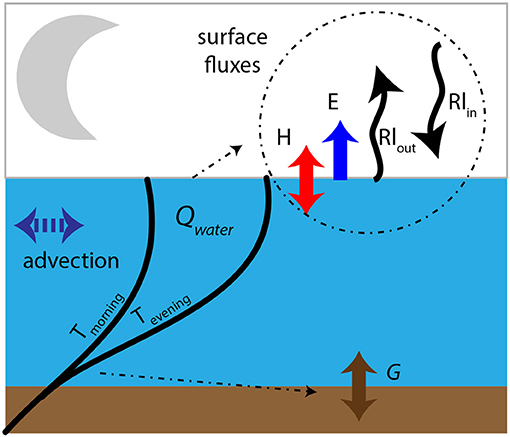
Figure 2. Schematic representation of all heat fluxes influencing the balance of an urban pond at night. Q_water represents the heat released by the pond over night as defined by integrating over the temperature change between evening (T_evening) and morning (T_morning) temperature. We define upward turbulent fluxes (E and H) as positive and downward as negative. Ground flux (G) and the net radiation are defined as positive in downward direction. This is consistent with the consensus of flux sign based on its direction.

The net radiation energy flux over night was calculated as the difference between incoming and outgoing longwave radiation (R_net = Rl_in − Rl_out [Wm⁻²]). As Rl_in was always smaller than Rl_out above the pond at night, hence net radiation resulted in negative values. Shortwave radiation was considered, and confirmed by measurements, to be zero at night.

The sensible and latent heat flux can be derived from the Bowen ratio as follows:

$\begin{array}{ll}E=\frac{Q_{res}}{1+B}& (9)\end{array}$

$\begin{array}{ll}H=\frac{Q_{res}}{1+\frac{1}{B}}& (10)\end{array}$

Ground heat flux (G [Wm⁻²]) was calculated from the slope of the temperature gradient of the lowest 10 cm using

$\begin{array}{ll}G\approx K_{mud}\frac{\Delta T}{\Delta z}& (11)\end{array}$

where K_mud = 2.2 Wm⁻¹K⁻¹ is the thermal conductivity of wet soil [recommended estimate for when detailed information about the soil is not available; (Farouki, 1981)], Δz = 0.1 m, and ΔT is a temperature difference [K].

Advection was considered irrelevant most of the time due to stagnant water conditions. Potential exceptions are two nights with heavy rainfall (07/20 and 07/28) when there was an influx of cold water and a peak in water level.

3. Results

Figures 3a,b show the weather conditions at the measurement site. There is a gap in the dataset on 07/25 because of power failure. During the measurement period the conditions were mostly sunny with few cloudy days, and only two days with an overcast sky (07/21 and 08/06). Air temperatures varied between 15 and 34°C for daytime, and 15 and 27°C for night time (Figure 3b). Wind speed reached highest values at night, while during the day, the conditions were often windless with average wind of 0.3 ms⁻¹ (Figure 3a).

FIGURE 3

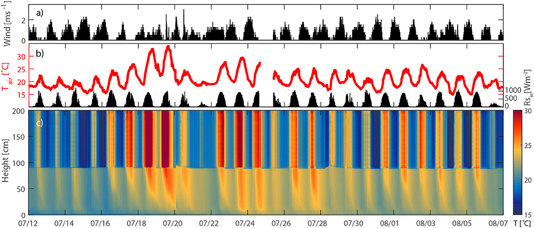
Figure 3. Measured variables for the whole period. (a) wind speed, (b) air temperature and radiation, 2 and 1.5 m above the water surface, respectively, (c) water and air temperature measured by the setup.

Figure 3c shows 5 min temperature measurements taken by the DTS setup for both water and air. Recorded profiles in both set-ups were very similar. A diurnal pattern is clearly visible for both air and water, although fluctuations in water temperature are not as strong. Increase in water level is visible after the two heavy rainfall events on 07/20 and 07/28.

In order to derive the latent and sensible heat flux using Equations 7 and 9, we needed to first calculate the radiative flux (R_net), the ground flux (G), and the net change in heat storage in the pond (Q_water). The resulting fluxes can be found in Figures 4a,b. The results in Table 1 show than on average 43% of the heat is lost through radiation and 7% is transferred downwards and stored in the muddy underlayer, leaving 50% of the energy available for turbulent fluxes (Q_res).

FIGURE 4

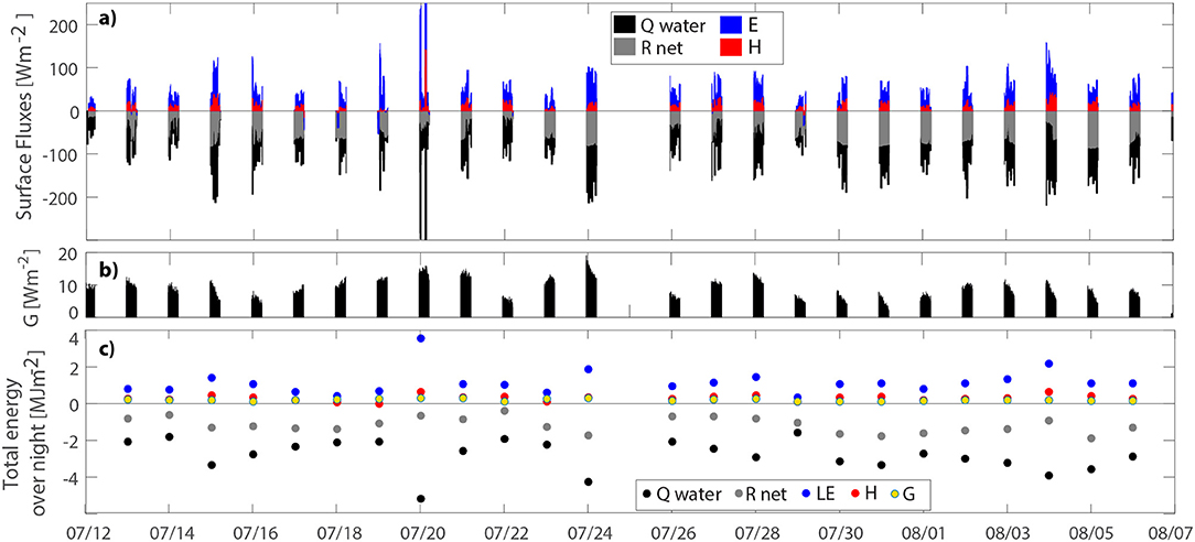
Figure 4. (a) Fluxes at the water surface in Wm⁻² at the night-time (23:00-05:00). E and H are positive in upward direction (from water to air), while Rl_net is positive in downward direction (from air to water) due to different definition of turbulent and radiative fluxes. (b) Ground flux from water to the bottom of the pond (positive in downward direction). (c) Sums of the different fluxes over each night in MJm⁻².

TABLE 1

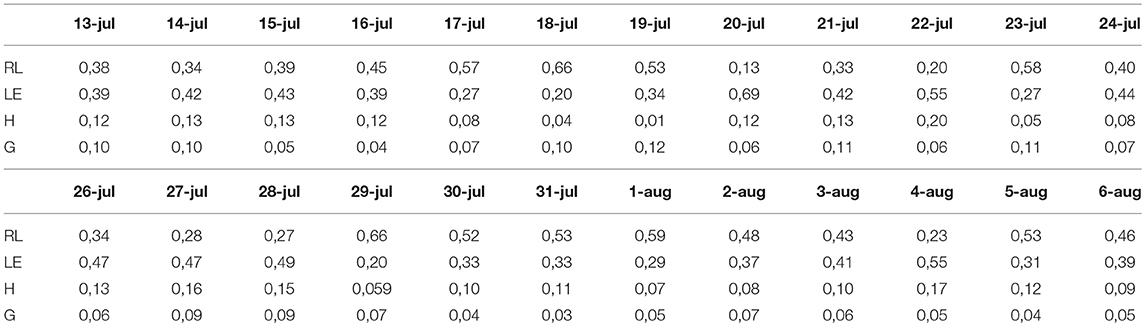
Table 1. Ratios of different fluxes with Q_water (flux/Q_water) for each day of the measurement period.

Second, the Bowen ratio was calculated (Figure 5). The nighttime values ranged form -0.07 and 0.46 with average of 0.27. The calculated values of sensible heat flux were, therefore, on average about four times smaller than latent heat flux, meaning that four times more heat was used for evaporation than was used for heating the air. The results suggest that, on average, 39% of the available energy was released by latent heat flux and only 11% in the form of sensible heat. Day-to-day ratio of the fluxes, however, varied. Sensible heat varied between 1% (07/19) and 20% (07/22). Latent heat flux made up between 20% (07/18) and 69% (07/20) of the total thermal energy emitted.

FIGURE 5

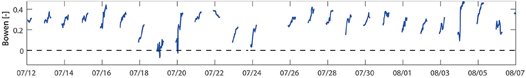
Figure 5. Bowen ration for night time.

The ratio of the turbulent and the radiative fluxes is strongly dependent on the meteorological conditions and climate of the location. For arid areas, the evaporative cooling can reach up to 57% of the total net cooling (Ali, 2007). Measured values of up to 69% of latent heat compared to other fluxes suggest that the warm dry air in the urban area can create a night-time oasis effect above an urban pond. The influence of meteorological conditions on Bowen ratio is easily visible during and after the heat wave (07/17 – 07/19). During the heat wave the Bowen ratio reaches the lowest values. This is due to increase in evaporation in combination with the relatively cold water surface compared to the air temperature; low sensible heat. Contrastingly, right after the heat wave, when the water temperature is relatively warm, the Bowen ratio peaks and stays relatively high during both day and night (07/20 – 07/22).

As Q_water resulted from integrating the temperature change over depth, temperature changes in deeper layers (Figures 6, 7a) of the pond provide an extra insight into the mechanism of night-time cooling of this urban pond and are vital for understanding the results presented in Figure 4. Both the instantaneous values of surface fluxes (Figure 4a), as well as the net temperature change overnight (Figure 4c), are dependent on the weather conditions during the previous day.

FIGURE 6

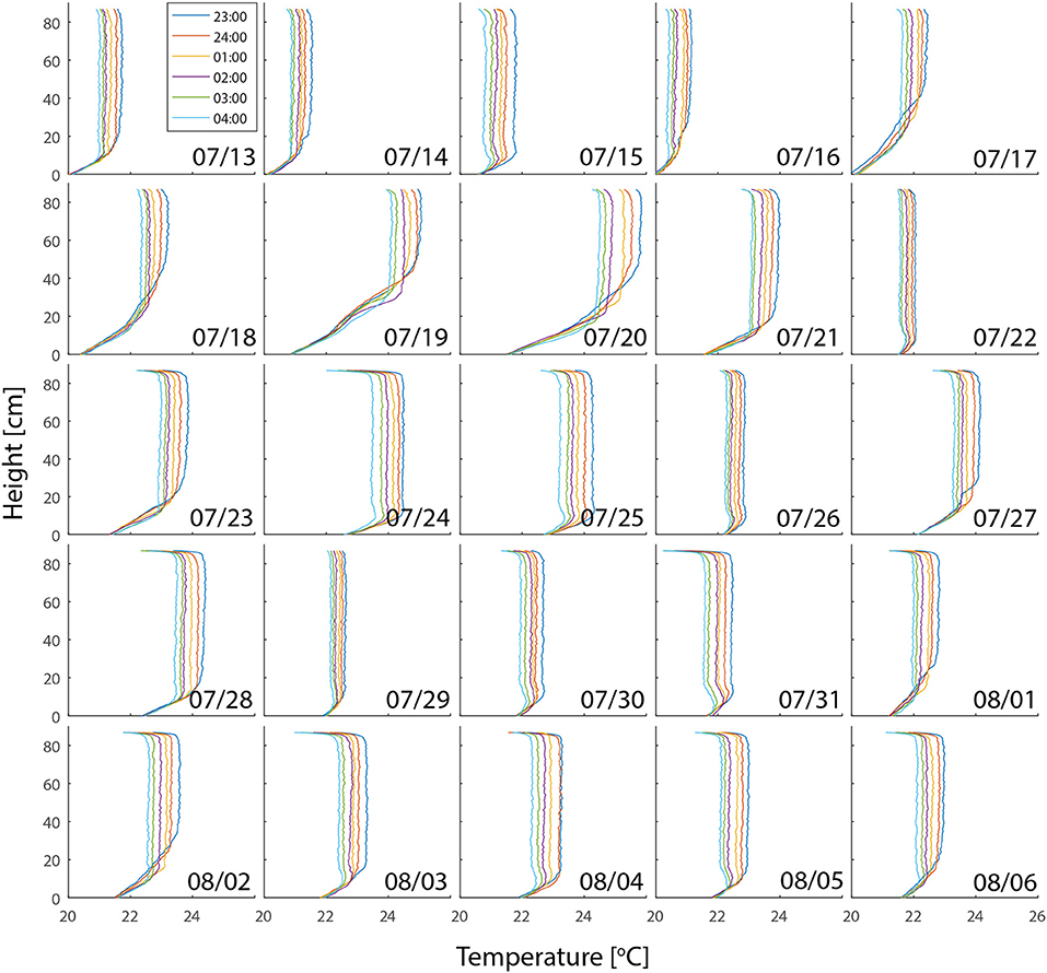
Figure 6. Instantaneous water temperature profiles at five different times each night of the measurement period. The night of 07/12–07/13 is annotated as 07/13 etc.

FIGURE 7

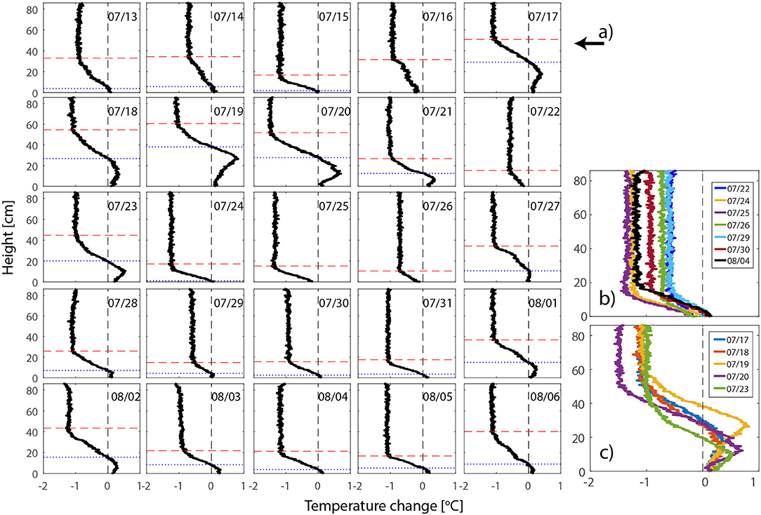
Figure 7. (a) Change in water temperature profile (T_morning– T_evening) for each day of the measurement period. Dashed line (red) shows location of the top well-mixed layer. Dotted line (blue) shows the depth at which the water experienced increase in temperature over the night. Subplot (b) shows examples of temperature profiles representing uniform change over the whole water depth with none or small increase of the bed sediment temperature, and subplot (c) shows examples of temperature profiles with net temperature increase in the lower water levels. All profiles start at the bottom of the lake (h = 0) and end at the water level (h = 86 cm).

The type of profile typical for nights following a relatively cloudy or cold day is shown in Figure 7b. Water temperature change during these nights was gradual and equal for the whole profile. Close to the bottom of the lake, where the muddy layer begins (ca 10–15 cm from the bottom), the temperature was more stable and did not change much in the course of one night. The surface energy balance during such nights occasionally resulted in negative latent and sensible heat flux values for the last hour of the night (e.g., 07/29). This was caused by the assumption of energy balance closure on hourly basis, and the combination of only small decrease in water temperature (Q_water) and longwave radiation being still relatively high.

Second type of net temperature change profile (Figure 7c) usually follows warm days with a clear sky, for example 07/18 (Figure 3). High turbidity of the water in the pond caused that only about half of the water profile experienced increase in temperature during the day. This resulted in a high temperature difference between the top layer (25.2°C) and the bottom layer (20.8°C) of the water at the beginning of the night. Energy for heating up the lower layers of water and the bed sediment was extracted from the top layer of water leaving less energy available to be released to the air. This situation is mainly visible during the first hour of the night, when the total temperature change in the water profile (Q_water) is close to zero, while the net longwave radiation is about –50 Wm⁻². As energy balance closure is assumed over each hour, the surface fluxes distribution in Figure 4a shows a negative sensible and latent heat flux. A similar, but more extreme, situation is visible also the following night (07/20).

The bottom 10 centimeters of the temperature profile represent the bed of the pond. Figure 6 shows that the bottom of the pond had always the lowest temperature of the whole profile. The lowest 10 cm of the profile always experienced a temperature gradient from warmer layers above, to the cold bottom of the pond. Above the lowest 10 cm was a transition layer of loose mud that functioned as a temperature buffer. This buffering is clearly visible in temperature profiles from nights following cold cloudy days (especially 07/31, Figure 6). In the evening of those nights, the buffer layer had a temperature similar to the water, but did not cool at the same rate, staying relatively warm compared to both the water and the bed. This difference in thermal behavior of this layer is probably caused by different composition of the mud with a high percentage of decomposing organic matter.

4. Discussion

The Bowen ratio used in this research (Equation 1) assumes equal transfer coefficients for water vapor and heat, which may not be a valid assumption away from neutral conditions. This is known as the β closure method (Green et al., 1994) and has been widely used (e.g., Hoedjes et al., 2002; Solignac et al., 2009; McJannet et al., 2011; Schilperoort et al., 2018). This method assumes that the air temperature is measured above the water surface, close enough not to be influenced by other variables (Bink, 1996), which was the case for this research. Relatively homogeneous air temperature profiles above water level are also visible in Figure 3c.

Uncertainty in the ground flux calculation is introduced by the choice of thermal conductivity of wet soil. 2.2 Wm⁻¹K⁻¹ is a value commonly used, when soil analysis is not possible (Farouki, 1981), however the values of thermal conductivity of wet soil vary between 1.5 and 2.5 Wm⁻¹K⁻¹ (Kersten, 1949; Johansen, 1977; Côté and Konrad, 2005), or even up to 6 Wm⁻¹K⁻¹ for saturated quartz sands (Zhang et al., 2015). Increasing the thermal conductivity of the mud to the highest value found in literature, will increase the ground flux by approximately factor 3. However, ground flux is likely to stay the smallest of all components.

Situations when the calculated latent heat flux resulted in negative values very well represent the weakness of using Bowen ratio and energy balance at an hourly basis to calculate turbulent fluxes. Assuming that the heat (temperature) change over the whole depth will be the same as the sum of the outgoing fluxes is valid when considering the whole night period. On hourly basis, this method can lead to unreasonable results. One hour time step was chosen as a compromise between the need to have as short time steps as possible to ensure validity of Bowen ratio, and the need to take as long time step as possible to ensure that the temperature change over the whole water depth will be representative to the heat released. Hourly averages are often used by authors to estimate turbulent fluxes (e.g., Sene et al., 1991; Meijninger and De Bruin, 2000).

The hourly closure can pose a problem especially after extremely sunny and warm days for highly turbid waters. When heat is not evenly distributed over the depth and the top layer of water is much warmer than water below, the calculation will result in negative values for latent heat flux (07/18). Besides negative latent heat flux, the calculation can also result in extreme values. For example, at 03:05 on 07/20 the calculated latent heat flux peaked to a false 630 Wm⁻². This sudden bias was caused by extreme temperature drop during that hour related to influx of cold rain water. This is why this outlier was removed from the dataset used to calculate the average fluxes. A more detailed modeling of the energy fluxes in the water would be required to get better estimates of the turbulent energy fluxes for these exceptional nights.

Despite the above described weaknesses, the energy balance method provides an reasonable estimate for calculation of surface energy fluxes, certainly when integrated over the whole night instead of hourly energy balances. It does not require a complex model that would calculate the fluxes under unstable atmospheric conditions. Nonetheless, due to its weaknesses, it is always necessary to take into account the whole picture. Combination of Figures 4a,c with the profiles in Figures 6, 7 provides a comprehensive story about how heat leaves an urban pond at night. It is necessary to take into account all the aspects that can influence the energy balance of the pond in order to avoid misinterpretations of the data.

There are very few quantitative studies, none focusing explicitly on night time effects to our knowledge. Oswald et al. (2012) show a weak correlation between distance to a large water body and air temperature in Detroit. Areas within 6 km showed a higher low temperature (+0.5°C) and a slightly lower high temperature (–0.3°C) than areas further away. Although this setting is not directly comparable to that of the small urban setting studied here, a general dampening of extremes was observed in both cases. The second relevant study is (Theeuwes et al., 2013), which used detailed modeling of a general urban setting with and without an idealized lake in an urban. Temperature differences of up to 2°C were simulated for the situation with and without water present. Temperature at 6:00 was up to 2°C higher when water was present compared to the situation where no water was present. However, this study was purely based on numerical simulations under idealized (windy) conditions. For example, the distribution of temperature over the water column due to turbidity was not taken into account, while this seems to be central to our case where night time warming is relatively small.

Here presented research showed that only 11% of the heat released influences the air temperature. Further studies should focus on comparing these findings to energy balances of different urban surfaces. Water is known to have high thermal inertia which causes slower release of the stored heat, this results in water being the warmest surface by the end of the night.

5. Conclusion

This paper analyzed data from a measurement campaign in a shallow urban pond in Delft, The Netherlands, in the summer of 2014 in order to assess the energy balance of such an urban surface water during hot summer nights. Previous research has shown that water bodies at night have the highest surface temperature of all the urban surfaces (Theeuwes et al., 2013; Yang and Zhao, 2015; Syafii et al., 2016), and therefore act as a heating element of the city. The results of this study show that, on an average hot summer night, radiative cooling (43 ±14%) and latent heat flux (39 ±11%) are the predominant ways the heat escapes the water body. Sensible heat flux, which is the only one that increases the air temperature, made up to just around 11% (±4%) of all the energy released by the pond at night. The remaining 7% (±2%) was drained into the bed sediment.

Weather conditions of the preceding day have a strong effect on the temperature distribution in the water column and on the cooling of the pond the night after. During warm days with high incoming solar radiation (e.g., 07/17–07/19), the high turbidity of the pond caused the upper layers of water to become much warmer (up to 5°C) than the water temperature near the bed. At night, this warm top layer predominantly heated the underlying water and the effect on the air was therefore minimal. Cold cloudy days resulted in smaller increases in water temperature and a more uniform temperature profile in the evening.

Lowest 10–15 cm of the measured profile was in the mud on the bottom of the pond. The deepest point measured in this campaign was the coldest point of the night-time profiles for all days and the lowest 10 cm of mud always experienced a temperature gradient suggesting a heat flux from water to the bed. This ground flux was estimated to range between 0.10 and 0.32 MJm⁻² per night but uncertainty in the thermal conductivity of the bed sediment is large.

This paper confirms the previously found heating effect of open water bodies at night for moderate climate cities (Oswald et al., 2012; Theeuwes et al., 2013). On top of that, we have shown that although an urban water body is a hot spot during nighttime, only around a tenth of the heat is released in a form that directly influences the air temperature. Small water bodies are notoriously difficult to generalize; even more so if their surroundings are as heterogeneous as urban landscape. Therefore, a body of case studies needs to be developed to fully understand how precisely do small water bodies influence urban climate, both during day- and nighttime. When this goal is reached, findings of this paper can further contribute to more appropriate and better informed use of open water in urban areas. Additionally, the data set is freely available and can already be used for validation of urban climate models (Solcerova et al., 2017).

Author Contributions

AS designed measurement setup and experiments, performed experiments and wrote the initial paper. AS, FvdV, and NvdG analyzed data and contributed to writing the paper.

Funding

Funding for this research was provided by research project Blue-Green Dream and the Climate KIC organization.

Conflict of Interest Statement

The authors declare that the research was conducted in the absence of any commercial or financial relationships that could be construed as a potential conflict of interest.

Acknowledgments

This research is part of a Climate KIC research project Blue-Green Dream, investigating the cooling effects of blue-green climate adaptation measures in urban areas. All data can be obtained from 4TU Center for Research Data.

Supplementary Material

The Supplementary Material for this article can be found online at: https://www.frontiersin.org/articles/10.3389/feart.2019.00156/full#supplementary-material

References

Abbasi, A., Annor, F. O., and van de Giesen, N. (2017). Effects of atmospheric stability conditions on heat fluxes from small water surfaces in (semi-) arid regions. Hydrol. Sci. J. 62, 1422–1439. doi: 10.1080/02626667.2017.1329587

CrossRef Full Text | Google Scholar

Albers, R., Bosch, P., Blocken, B., van den Dobbelsteen, A., van Hove, L., Spit, T., et al. (2015). Overview of challenges and achievements in the climate adaptation of cities and in the climate proof cities program. Build. Environ. 83, 1–10. doi: 10.1016/j.buildenv.2014.09.006

CrossRef Full Text | Google Scholar

Ali, A. H. H. (2007). Passive cooling of water at night in uninsulated open tank in hot arid areas. Energy Conver. Manage. 48, 93–100. doi: 10.1016/j.enconman.2006.05.012

CrossRef Full Text | Google Scholar

Barr, A. G., King, K., Gillespie, T., Den Hartog, G., and Neumann, H. (1994). A comparison of bowen ratio and eddy correlation sensible and latent heat flux measurements above deciduous forest. Bound. Layer Meteorol. 71, 21–41. doi: 10.1007/BF00709218

CrossRef Full Text | Google Scholar

Bink, N. (1996). The ratio of eddy diffusivities for heat and water vapour under conditions of local advection. Phys. Chem. Earth 21, 119–122.

Google Scholar

Bowen, I. S. (1926). The ratio of heat losses by conduction and by evaporation from any water surface. Phys. Rev. 27:779.

Google Scholar

Côté, J., and Konrad, J.-M. (2005). A generalized thermal conductivity model for soils and construction materials. Can. Geotechn. J. 42, 443–458. doi: 10.1139/t04-106

CrossRef Full Text | Google Scholar

Coutts, A. M., Tapper, N. J., Beringer, J., Loughnan, M., and Demuzere, M. (2012). Watering our cities: The capacity for water sensitive urban design to support urban cooling and improve human thermal comfort in the australian context. Progress Phys. Geogr. 37, 2–28. doi: 10.1177/0309133312461032

CrossRef Full Text | Google Scholar

CPC-Consortium (2014). Eindreport Climate Proof Cities 2010-2014. CPC-Consortium

Farouki, O. T. (1981). Thermal Properties of Soils. Technical report, DTIC Document.

Google Scholar

Gago, E. J., Roldan, J., Pacheco-Torres, R., and Ordonez, J. (2013). The city and urban heat islands: a review of strategies to mitigate adverse effects. Renew. Sustain. Energy Rev. 25, 749–758. doi: 10.1016/j.rser.2013.05.057

CrossRef Full Text | Google Scholar

Green, A., McAneney, K., and Astill, M. (1994). Surface-layer scintillation measurements of daytime sensible heat and momentum fluxes. Bound. Layer Meteorol. 68, 357–373.

Google Scholar

Halper, E. B., Scott, C. A., and Yool, S. R. (2012). Correlating vegetation, water use, and surface temperature in a semiarid city: A multiscale analysis of the impacts of irrigation by single-family residences. Geograph. Analys. 44, 235–257. doi: 10.1111/j.1538-4632.2012.00846.x

CrossRef Full Text | Google Scholar

Hathway, E. A., and Sharples, S. (2012). The interaction of rivers and urban form in mitigating the urban heat island effect: a uk case study. Build. Environ. 58, 14–22. doi: 10.1016/j.buildenv.2012.06.013

CrossRef Full Text | Google Scholar

Hicks, B. B. (1975). A procedure for the formulation of bulk transfer coefficients over water. Bound. Layer Meteorol. 8, 515–524.

Google Scholar

Hilgersom, K., Van Emmerik, T., Solcerova, A., Berghuijs, W., Selker, J., and Van de Giesen, N. (2016). Practical considerations for enhanced-resolution coil-wrapped distributed temperature sensing. Geosci. Instrum. Method. Data Syst. 5, 151–162. doi: 10.5194/gi-5-151-2016

CrossRef Full Text | Google Scholar

Hoedjes, J., Zuurbier, R., and Watts, C. (2002). Large aperture scintillometer used over a homogeneous irrigated area, partly affected by regional advection. Bound. Layer Meteorol. 105, 99–117. doi: 10.1023/A:1019644420081

CrossRef Full Text | Google Scholar

Johansen, O. (1977). Thermal Conductivity of Soils. Technical report, DTIC Document.

Google Scholar

Kersten, M. S. (1949). Laboratory Research for the Determination of the Thermal Properties of Soils. Technical report, DTIC Document.

Google Scholar

Lee, H.-Y. (1993). An application of noaa avhrr thermal data to the study of urban heat islands. Atmosph. Environ. Part B. Urban Atmos. 27, 1–13.

Google Scholar

Manteghi, G., bin Limit, H., and Remaz, D. (2015). Water bodies an urban microclimate: a review. Modern Appl. Sci. 9:1. doi: 10.5539/mas.v9n6p1

CrossRef Full Text | Google Scholar

McJannet, D., Cook, F., McGloin, R., McGowan, H., and Burn, S. (2011). Estimation of evaporation and sensible heat flux from open water using a large-aperture scintillometer. Water Res. Res. 47:W05545. doi: 10.1029/2010WR010155

CrossRef Full Text | Google Scholar

Meijninger, W., and De Bruin, H. (2000). The sensible heat fluxes over irrigated areas in western turkey determined with a large aperture scintillometer. J. Hydrol. 229, 42–49. doi: 10.1016/S0022-1694(99)00197-3

CrossRef Full Text | Google Scholar

Oke, T. R. (1982). The energetic basis of the urban heat island. Quart. J. R. Meteorol. Soc. 108, 1–24.

Google Scholar

Oke, T. R., Johnson, G. T., Steyn, D. G., and Watson, I. D. (1991). Simulation of surface urban heat islands under ‘ideal’ conditions at night part 2: diagnosis of causation. Bound. Layer Meteorol. 56, 339–358.

Google Scholar

Olah, A. B. (2012). The possibilities of decreasing the urban heat island. Appl. Ecol. Environ. Res. 10, 173–183. doi: 10.15666/aeer/1002-173183

CrossRef Full Text | Google Scholar

Oswald, E. M., Rood, R. B., Zhang, K., Gronlund, C. J., O'Neill, M. S., White-Newsome, J. L., et al. (2012). An investigation into the spatial variability of near-surface air temperatures in the detroit, michigan, metropolitan region. J. Appl. Meteorol. Climatol. 51, 1290–1304. doi: 10.1175/JAMC-D-11-0127.1

CrossRef Full Text | Google Scholar

Patz, J. A., Campbell-Lendrum, D., Holloway, T., and Foley, J. A. (2005). Impact of regional climate change on human health. Nature 438, 310–317. doi: 10.1038/nature04188

PubMed Abstract | CrossRef Full Text | Google Scholar

Rinner, C., and Hussain, M. (2011). Toronto's urban heat island - exploring the relationship between land use and surface temperature. Remote Sens. 3, 1251–1265. doi: 10.3390/rs3061251

CrossRef Full Text | Google Scholar

Ryu, Y.-H., and Baik, J.-J. (2012). Quantitative analysis of factors contributing to urban heat island intensity. J. Appl. Meteorol. Climatol. 51, 842–854. doi: 10.1175/JAMC-D-11-098.1

CrossRef Full Text | Google Scholar

Schilperoort, B., Coenders-Gerrits, M., Luxemburg, W., Jiménez Rodríguez, C., Cisneros Vaca, C., and Savenije, H. (2018). Using distributed temperature sensing for bowen ratio evaporation measurements. Hydrol. Earth Syst. Sci. 22, 819–830. doi: 10.5194/hess-22-819-2018

CrossRef Full Text | Google Scholar

Selker, J. S., Thevenaz, L., Huwald, H., Mallet, A., Luxemburg, W., Van De Giesen, N., et al. (2006). Distributed fiber-optic temperature sensing for hydrologic systems. Water Res. Res. 42:W12202. doi: 10.1029/2006WR005326

CrossRef Full Text | Google Scholar

Sene, K., Gash, J., and McNeil, D. (1991). Evaporation from a tropical lake: comparison of theory with direct measurements. J. Hydrol. 127, 193–217.

Google Scholar

Solcerova, A., Emmerik, T. v., Ven, F. v. d., Selker, J., and Giesen, N. v. d. (2018). Skin effect of fresh water measured using distributed temperature sensing. Water 10:214. doi: 10.3390/w10020214

CrossRef Full Text | Google Scholar

Solcerova, A., van de Ven, F., and van de Giesen, N. (2017). Water and Air Temperature at Amalia van Solmslaan Pond, Delft, 2014. TU Delft. doi: 10.4121/uuid:7cdcab96-aea2-48b2-939b-9eb67b3532f3

CrossRef Full Text

Solignac, P. A., Brut, A., Selves, J.-L., Béteille, J.-P., Gastellu-Etchegorry, J.-P., Keravec, P., et al. (2009). Uncertainty analysis of computational methods for deriving sensible heat flux values from scintillometer measurements. Atmos. Measure. Techn. 2, 741–753. doi: 10.5194/amt-2-741-2009

CrossRef Full Text | Google Scholar

Steeneveld, G. J., Koopmans, S., Heusinkveld, B. G., and Theeuwes, N. E. (2014). Refreshing the role of open water surfaces on mitigating the maximum urban heat island effect. Land. Urban Plann. 121, 92–96. doi: 10.1016/j.landurbplan.2013.09.001

CrossRef Full Text | Google Scholar

Syafii, N. I., Ichinose, M., Wong, N. H., Kumakura, E., Jusuf, S. K., and Chigusa, K. (2016). Experimental study on the influence of urban water body on thermal environment at outdoor scale model. Proc. Eng. 169, 191–198. doi: 10.1016/j.proeng.2016.10.023

CrossRef Full Text | Google Scholar

Tan, J., Zheng, Y., Song, G., Kalkstein, L., Kalkstein, A., and Tang, X. (2007). Heat wave impacts on mortality in shanghai, 1998 and 2003. Int. J. Biometeorol. 51, 193–200. doi: 10.1007/s00484-006-0058-3

PubMed Abstract | CrossRef Full Text | Google Scholar

Theeuwes, N. E., Solcerova, A., and Steeneveld, G. J. (2013). Modeling the influence of open water surfaces on the summertime temperature and thermal comfort in the city. J. Geophys. Res. Atmosph. 118, 8881–8896. doi: 10.1002/jgrd.50704

CrossRef Full Text | Google Scholar

Tyler, S. W., Selker, J. S., Hausner, M. B., Hatch, C. E., Torgersen, T., Thodal, C. E., et al. (2009). Environmental temperature sensing using raman spectra dts fiber-optic methods. Water Res. Res. 45. doi: 10.1029/2008WR007052

CrossRef Full Text | Google Scholar

Wang, Z. H., Lu, J., Xie, L., and Chen, S. L. (2011). “Study on heat island effect of Chongqing in summer,” in 7th International Symposium on Heating, Ventilating and Air Conditioning - Proceedings of ISHVAC 2011, Vol. 2, 588–593.

Wen-Yao, L., Field, R., Gantt, R., and Klemas, V. (1987). Measurement of the surface emissivity of turbid waters. Remote Sens. Environ. 21, 97–109.

Google Scholar

Xu, J., Wei, Q., Huang, X., Zhu, X., and Li, G. (2010). Evaluation of human thermal comfort near urban waterbody during summer. Build. Environ. 45, 1072–1080. doi: 10.1016/j.buildenv.2009.10.025

CrossRef Full Text | Google Scholar

Yang, X., and Zhao, L. (2015). Diurnal thermal behavior of pavements, vegetation, and water pond in a hot-humid city. Buildings 6:2. doi: 10.3390/buildings6010002

CrossRef Full Text | Google Scholar

Zhang, N., Yu, X., Pradhan, A., and Puppala, A. J. (2015). Thermal conductivity of quartz sands by thermo-time domain reflectometry probe and model prediction. J. Mater. Civil Eng. 27:04015059. doi: 10.1061/(ASCE)MT.1943-5533.0001332

CrossRef Full Text | Google Scholar