 Max Berkelhammer
- Department of Earth and Environmental Sciences, University of Illinois at Chicago, Chicago, IL, United States
The primary productivity of adjacent terrestrial and marine ecosystems can display synchronous responses to climate variability. Previous work has shown that this behavior emerges along the California coast where internal modes of climate variability, such as El Niño Southern Oscillation (ENSO) and the Pacific Decadal Oscillation (PDO), alter jet stream dynamics that influence marine ecosystems through changes in upwelling and terrestrial ecosystems through changes in precipitation. This study assesses whether marine-terrestrial synchrony is a widespread phenomenon across the North Pacific by utilizing satellite-derived Solar-Induced Fluorescence (SIF) and chlorophyll-α as proxies for land and sea productivity, respectively. The results show that terrestrial and marine ecosystems are consistently synchronized across 1000's of kms of the North Pacific coastline. This synchrony emerges because both marine and terrestrial ecosystems respond to climate modes with a similar north-south dipole pattern that is mirrored across the coastal interface. The strength of synchrony is modulated by the relative states of the PDO and ENSO because the terrestrial north-south dipole is strongly controlled by the PDO while the marine pattern follows ENSO. The consequence is marine and terrestrial productivity anomalies that are opposite one another along adjacent regions of the coastline. If ENSO and the PDO have shared low-frequency variance, then synchrony would be the dominant state despite local topographic and trophic diversity along the coastlines. This result suggests that climate proxy stacks that include biologically sensitive marine and terrestrial proxies would have a selective sensitivity to modes such as PDO that drive synchrony. Lastly, the coupling of land and sea productivity may have the effect of generating amplified regional responses of the carbon budget to climate variability by simultaneously enhancing the terrestrial and marine carbon sinks.
1. Introduction
Climate variability drives synchronous responses in ecosystems over large spatial domains. This effect has been well-illustrated through the tree ring network from the western US that shows spatially coherent interannual and decadal variations in tree growth (Cook et al., 2007; Fang et al., 2018). The ecological response to climate variability may also “straddle” both terrestrial and aquatic systems and generate synchronous responses across the coastal interface. This is, in fact, an assumption embedded in multi-proxy climate reconstructions that incorporate biologically-sensitive proxies from land, lake and marine systems (e.g., Abram et al., 2016). It is difficult to assess the strength and/or persistence of the terrestrial-aquatic synchrony because records such as tree rings or sediment cores are not continuous across the land-sea interface and because both age uncertainty and/or differences in the timescale of proxy response functions may obscure the presence or absence of coupled behavior. An explicit assessment of this phenomenon was done by Guyette and Rabeni (1995), who found significant correlation between the annual growth rings of trees and stream fish in the Ozark region of the US. The species share a common response to summer rainfall, which affected water availability for the trees and nutrient availability for the fish. Ong et al. (2016) extended this type of analysis to the regional scale by analyzing the common responses of corals, trees and fish across NW Australia using overlapping growth chronologies from this collection of both marine and terrestrial taxa. The authors found a common response of all species to El Niño (ENSO) through its effect on regional rainfall and SSTs. In another example from this region, Ruthrof et al. (2018) found that in response to a significant 2011 heat wave in western Australia, there was ecological collapse that straddled the coastal land and sea ecosystems leading to both widespread tree morality and coral bleaching. As illustrated by these studies in western Australia, the increase in the frequency of heat waves and potential for increased variance in ENSO with global warming has the capacity to drive greater degrees of synchrony (Rosenzweig et al., 2008; Hoegh-Guldberg and Bruno, 2010).
The North Pacific serves as an interesting domain to consider the mechanisms and pervasiveness of aquatic and terrestrial synchrony. It is a region that experiences high amplitude climate variability at a variety of timescales associated with ENSO, the Pacific Decadal Oscillation (PDO) and the Arctic Oscillation (AO) (Cayan et al., 1999; Smith and Sardeshmukh, 2000; Mantua and Hare, 2002; Newman et al., 2003; Wise, 2016), all of which have documented effects on both marine (Karl et al., 1995; Mantua et al., 1997; Fisher et al., 2015; Lindegren et al., 2018) and terrestrial ecosystems (Biondi et al., 2001; Trouet and Taylor, 2010; McCabe et al., 2012). Black et al. (2014) and Black et al. (2018) undertook a series of studies that focused on common responses between the terrestrial ecosystems in California and the marine systems in the adjacent coastal upwelling zone. Marine primary productivity along the coast is strongly tied to wind-driven upwelling (Jacox et al., 2015; García-Reyes et al., 2018), which is affected by the wintertime high pressure patterns in the North Pacific. It is these same pressure patterns that influence winter precipitation and growing season soil moisture, which limit terrestrial primary productivity and tree growth. Consequently, coherence between terrestrial and aquatic ecosystems arises through the ubiquitous effects of these atmospheric circulation patterns on regional climate (e.g., rainfall, snowpack, wind fields and temperature). By utilizing a combination of blue oak tree ring chronologies, otolith growth-increment chronologies, records of sea-bird egg laying dates and breeding success, the studies by Black et al. were able to identify synchronous behavior tied to a common wintertime atmospheric blocking pattern (Wise, 2016). As in the case of northwestern Australia (Ong et al., 2016), the periods of strongest synchrony were correlated with large ENSO events.
The aforementioned work on this topic has primarily considered synchrony in terms of coincident changes in individual aquatic and terrestrial species (e.g., blue oak or rock fish). The results have thus emphasized this phenomenon in terms of its ecological impacts, namely that changes in breeding success or mortality events could produce cascading trophic changes (Black et al., 2018). The work presented here builds from the concepts of these previous studies but seeks to assess the generality of terrestrial-marine synchrony by utilizing satellite-derived indicators of primary productivity or changes in biomass. Through the use of satellite indices, the analysis is able to consider the spatial extent of synchrony over an area of 1000's of km and test whether synchrony manifests at the scale of grid-averaged primary productivity as opposed to the response of individual species. The work is intended to expand upon the known ecological implications of terrestrial and aquatic synchrony by considering whether coherence between terrestrial and aquatic productivity might also influence interannual or decadal variability in the global carbon budget (Le Quéré et al., 2012). The motivation for this analysis is that there is significant interannual and decadal variability in the global carbon budget associated with climatic-driven variations in the terrestrial (Poulter et al., 2014; Ahlström et al., 2015) and oceanic (Eddebbar et al., 2017) carbon sinks, which can influence the rate that CO2 accumulates in the atmosphere in spite of the dominant trend associated with anthropogenic emissions (Ballantyne et al., 2012). Understanding the temporal variability of these surface carbon sink terms is critical for the development of robust carbon cycle models (Landschuetzer et al., 2016; Li et al., 2016). If terrestrial and aquatic carbon cycles are tightly coupled, this could exacerbate the effects of climate modes on variability of the global carbon budget. On the other hand, if productivity between land and sea is decoupled or asynchronous, it could have the effect of buffering the role of ocean-atmosphere climate modes (such as ENSO) on the carbon budget.
Besides potential impacts of land-ocean coupling on the global carbon budget, synchrony is also a critical aspect of the climate signal stored in multi-proxy climate reconstructions that incorporate biotic proxies from terrestrial, lacustrine and marine systems (e.g., Ahmed et al., 2013). If certain modes of climate variability have synchronous effects across the aquatic and terrestrial interface, then these modes would be strongly represented in the proxy record. For example, the aforementioned study by Guyette and Rabeni (1995) from the Ozarks showed that summer rainfall influenced both fish and tree growth whereas the trees were influenced by summer temperatures and the fish by winter temperatures. From this example, it is possible to envision how a simple proxy stack using these two records would accentuate the rainfall signal while losing the specific information on temperature seasonality within the individual records. Aspects of this problem have been discussed in the context of comparisons between lake and tree ring records by Steinman et al. (2014) who noted discrepancies between these proxies may be the result of the tree rings' sensitivity to summer moisture and the lakes' sensitivity to winter moisture. There has already been significant work on the issue of proxy seasonality and how it can be addressed within multi-proxy syntheses (e.g., Abram et al., 2016) and the analyses presented here takes a general look at this issue by quantifying the response of regional land and marine productivity to North Pacific climate modes.
The study utilizes three types of analyses applied to satellite retrievals of solar-induced fluorescence and chlorophyll-α to illustrate synchrony between marine and terrestrial ecosystems in the North Pacific. In the first part of the paper, an EOF analysis is applied to both the terrestrial, marine and a joint terrestrial and marine matrix to identify the dominant spatiotemporal modes of variability and their respective drivers (i.e., section Spatio-Temporal Patterns of Productivity and Figures 1, 3–6). In the second part of the paper, specific years are discussed (2015, 2012 and 2009), which highlight the signature and potential climate mechanisms that drive synchronous behavior (i.e., Section Case Studies of 2009, 2012, and 2015 and Figures 6, 7) and the paper concludes with a regression analysis between adjacent coastal and marine indices of productivity to specifically assess the spatial signature of terrestrial-aquatic synchrony (Section Spatial Analysis of Synchrony from Regression Analysis and Figure 8).
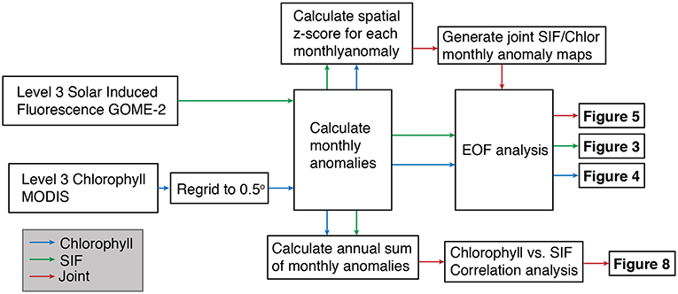
Figure 1. Diagram showing workflow of analyses and the respective figures produced through these analyses.
2. Materials and Methods
2.1. Spatial Domain
This study focuses on a domain bounded between 30° and 65°N latitude and −180° to –110 °W longitude. This area was chosen to encompass the eastern half of the North Pacific Basin and western North America. As opposed to previous work done in this region and elsewhere (Guyette and Rabeni, 1995; Black et al., 2014; Ruthrof et al., 2018), the intent was to select a large region associated with diverse marine and terrestrial ecoregions to assess the maximum scale at which synchronous behavior might be expected. The northern boundary of the domain was defined by the interface between the Pacific and Arctic oceans. While the western boundary is somewhat arbitrary, the vast majority of the chlorophyll variance occurs along the coastal margin and thus the results were not sensitive to the western boundary choice (Messié and Chavez, 2011). The terrestrial domain includes xeric regions in the southwestern US, hydric sites along the coastal ranges and arctic sites in Alaska. The consequence of including such a large terrestrial domain is that a single dominant limiting factor for productivity such as summer rainfall or radiation was not present.
2.2. Satellite and Reanalysis Datasets
2.2.1. Solar-Induced Fluorescence
Solar-Induced Fluorescence (SIF) is emitted as a byproduct of photosynthesis with two predominant peaks centered near 685 and 740 nm. A number of satellite platforms are now capable of retrieving SIF and this study uses data from the Global Ozone Monitoring Experiment 2 (GOME-2), which is flown on the MetOp-A satellite (Joiner et al., 2013). The native spatial resolution of the data was 40 × 80 km until 2013 when the resolution was improved to 40 × 40 km. The SIF retrievals used in this study are from the 734 to 758 nm window (i.e., the 740 nm peak). In this study, the Version 27 Level 3 data is used, which is a gridded product (0.5° × 0.5° grid) that has undergone some cloud filtering and bias correction (Joiner et al., 2014). We use data that covers January 2007 to December 2017, yielding 11 complete annual cycles. Further details of this dataset and how it was processed can be found in the following publications: Yang et al. (2015) and Joiner et al. (2013, 2014). This satellite product has already been applied toward analysis of spatial and temporal variability in terrestrial primary productivity in the western US forests (Berkelhammer et al., 2017), northern high latitude tundra (Luus et al., 2017) and high-latitude boreal forests (Jeong et al., 2017) and is therefore suitable for analysis of productivity within the domain of this study. No additional corrections or changes in projection/resolution were done to the data which is available from the Goddard Aura Validation Center (https://avdc.gsfc.nasa.gov/pub/data/satellite/MetOp/GOME_F/). We note that as opposed to other satellite indices of vegetation (such as NDVI), SIF is a retrieval of a rate-process (fluorescence emission) and is therefore a more direct proxy for primary productivity.
2.2.2. Chlorophyll-α
The analysis of marine productivity was undertaken using satellite retrievals of ocean chlorophyll from the MODerate-resolution Imaging Spectroradiometer (MODIS), which flies on the National Aeronautics and Space Administration (NASA) Earth Observing System (EOS). Data from the Aqua platform were used that has an early afternoon overpass. MODIS retrieves bandwidths from the following 7 channels: 620–670 (red), 841–876 (near infrared 1), 459–479 (blue), 545–565 (green), 1,230–1,250 (near infrared 2), 1,628–1,652 (short-wave infrared 1) and 2,105–2,155 nm (short-wave infrared 2). Surface chlorophyll-α concentrations in the units of mg m−3 are derived from an algorithm utilizing the green, blue and red bands that has been optimized through comparison with direct observations of chlorophyll (Hu et al., 2012). The analysis presented here is based on the Level 3 monthly product that is gridded onto a 4 km global grid over the period 2003–2017. This product and its predecessors have a long legacy for studies on analysis and modeling of marine ecosystem productivity. The satellite chlorophyll retrievals provide a robust proxy for phytoplankton biomass (e.g., Dore et al., 2008), which, in turn, has made them useful as inputs to models for marine primary productivity (Platt et al., 1991; Behrenfeld et al., 2006). We note that, unlike SIF, the chlorophyll data is an indicator of biomass concentration as opposed to primary productivity, which is a flux. Because of differences in photoefficiency, the chlorophyll retrievals cannot be taken as a linear and quantitative indicator of primary productivity. Nonetheless, we treat chlorophyll as a proxy for primary productivity (and refer to it as “marine productivity” hereafter), which is an assumption that is not always valid and one that limits the direct applicability of these results toward understanding the spatial structure of marine productivity and its influence on the strength of the carbon sink.
2.2.3. Supporting Climate Data
For analysis of climate conditions during specific years, data from NASA's modern-era retrospective analysis for research and applications (MERRA) was used (Rienecker et al., 2011). This is a reanalysis product that assimilates meteorological data and satellite retrievals to yield a global gridded estimate of the climate state on a global 0.5° latitude × 0.66° longitude grid. Comparisons of this reanalysis product and others (e.g., NCEP and ERA Interim) can be found in Rienecker et al. (2011). For this study, we utilize monthly resolved sea level pressure (Pa), 10 m U and V wind speeds (m s−1) and 2 m surface temperatures (K). In addition to the Reanalysis data, the spatiotemporal patterns in productivity were compared against the following climate modes: the Pacific Decadal Oscillation (PDO) (Mantua et al., 1997; Mantua and Hare, 2002), ENSO (specifically, the Oceanic Niño Index index) (Ropelewski and Halpert, 1986; Cayan et al., 1999; McCabe et al., 2004) and the Pacific North American pattern (PNA) (Trouet and Taylor, 2010). While this is not an exhaustive list of climate modes, these were the modes that produced the strongest correlation with the leading principal components of the different satellite products. Monthly timeseries for each of these datasets were accessed from National Ocean and Atmospheric Administration and all data were reported in normalized units. It is important to note that for PDO and ENSO, the strongest expression of the modes appears during the winter months. However, we found the strongest correlation between the climate modes and the satellite ecosystem indicators to emerge using the annual averages of the climate modes. We thus report and discuss the climate modes in terms of their annual averages, which has the effect of buffering their interannual variability by occasionally averaging periods that may include transitions from positive to negative states. There are multiple reasons why the correlations with productivity are stronger using the annual averages including that peak productivity occurs during spring and summer but may inherent legacy of the previous winter's conditions. In other words, spring wind fields might influence real time upwelling whereas wintertime anomalies in tropical Pacific SST might influence higher latitude thermocline conditions months later. Thus, there is ecological sensitivity to conditions over a longer seasonal window. While future work could benefit from exploring seasonal dynamics in the drivers of synchrony, for simplicity we hereafter discuss variability based on annual averaging.
2.3. Empirical Orthogonal Function Analysis
An Empirical Orthogonal Function (EOF) analysis was performed on monthly SIF and chlorophyll data from the domain bounded by 30° and 65°N latitude and –180° to –110 °W longitude. Both data were treated by subtracting the monthly climatological value at each grid cell to generate timeseries of monthly anomalies for each grid cell (Björnsson and Venegas, 1997) (Figure 1). For the individual analysis of the SIF and chlorophyll data, the data were not normalized by variance, which resulted in highly productive coastal regions having a larger weight on the analysis (Messié and Chavez, 2011). In order to generate a composite SIF/chlorophyll map, each of these datasets were normalized (as a spatial z-score) to produce a continuous land-sea productivity map. EOFs were then computed for the region, yielding a spatial pattern (i.e., an EOF) and a principal component (PC) time series that captured the temporal variability of each EOF mode. We consider only the first two EOFs for each analysis, which in all cases explained >50% of the variance. A calendar-year average for each of the PCs was then computed for comparison with the climate mode data. We note that the direction of the loading patterns is arbitrary, which becomes important when comparing the patterns that emerge from the individual EOF analyses (Figures 3, 4) with the joint EOF analysis (Figure 5).
2.4. Terrestrial-Aquatic Regression Analysis
To consider the spatial signature of terrestrial-aquatic synchrony, a linear regression analysis was performed between adjacent chlorophyll and SIF timeseries along each 0.5° region of the coastline. This was done by selecting all chlorophyll and SIF grid cells within 300 km of each coastal grid cell and computing an interannual average timeseries for the land and sea (Figure 1). The choice of 300 km is arbitrary but the analysis was largely insensitive to thresholds ranging from 200 to 500 km. The respective 300 km averaged land and sea timeseries were regressed against one another and a Pearson's correlation coefficient calculated. Synchrony was defined by coastal grid cells where the correlation coefficient was positive and the p < 0.1.
3. Results
3.1. Regional Patterns of Productivity and Seasonality
To provide context for the subsequent analyses, the regional patterns of chlorophyll and SIF seasonality and amplitude were assessed over the entire domain (Figure 2). Figure 2A shows the presence of high chlorophyll concentrations across the coastal regions and throughout the Arctic. At this scale, the complex pattern in the timing of peak productivity can be clearly observed (Figure 2B). The boundary between the southern and northern part of the Northeastern Pacific Basin is delineated by the North Pacific Current and observable by differences in chlorophyll seasonality such that the southern region has a peak in January and the northern region has a peak in September (Hurlburt et al., 1996). This current partially isolates the northern part of the basin affected by the Alaska and Kamchatka Currents (Figure 2). The chlorophyll peak in the intermediate zone between the north and south parts of the basin is poorly defined and is quite dynamic between years. The coastal regions of Alaska and the Pacific Northwest display a consistent chlorophyll maximum in May (Di Lorenzo et al., 2008; García-Reyes et al., 2018) while the timing of peak chlorophyll for the southern coastal regions are not spatially coherent. In terms of terrestrial productivity, SIF is maximum along the coastal mountains of the west coast of the US and across a region of high productivity in the plains of Canada that is an extension of the highly productive agricultural regions of the midwestern US (Hilton et al., 2017). Unlike chlorophyll, the terrestrial ecosystems are dominated by a wide homogenous region where peak productivity occurs in June and July. The exceptions can be found in the domain influenced by the North American Monsoon, that experiences its peak in productivity in August, and in parts of the Basin and Range region where peak productivity occurs in March (St. George et al., 2010; McCabe et al., 2012). These results are summarized by the histogram shown in Figure 2C, which illustrates the narrow and distinct distributions between the timing of peak productivity for terrestrial and coastal marine systems. In the North Pacific, the offset between the peak in terrestrial (July) and coastal marine (May) productivity is, on average, 2 months.
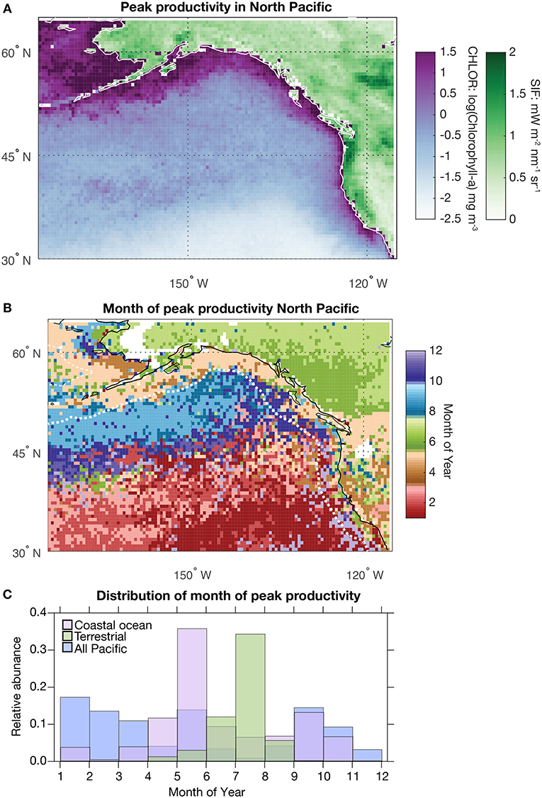
Figure 2. (A) Map showing the average of each year's maximum value for Solar-Induced Fluorescence (SIF) (greens) and chlorophyll-α (purples). (B) Map showing the average month that each grid cell reaches its peak in SIF and chlorophyll-α (as in A). The SIF data spans 2007–2017 and the chlorophyll-α data spans 2003–2017. Each dataset was gridded to a common 0.5° spatial resolution (Figure 1). (C) Distribution of the month of peak SIF and chlorophyll based on the data in (B). The coastal chlorophyll data includes all grid cells contained within the dotted white line shown in (B) (as in Figure 8).
3.2. Spatio-Temporal Patterns of Productivity
The EOF analysis of SIF identifies two dominant modes of variability that explain 34% and 24% of the variance (Figures 3A,C). The first of these modes is characterized by a strong dipole with a negative loading that runs along most of the west coast of the US and positive loadings along the coast of British Columbia and southern Alaska. The dipole is centered around a latitude of ~50° N. The PC of this EOF shows limited interannual variability and is highly correlated (r = 0.90) with annually-averaged PDO (Figure 3B). The effect of the PDO in generating a north-south dipole in tree ring widths in the western US has been identified elsewhere (e.g., MacDonald and Case, 2005) and the analysis presented here provides a spatially continuous depiction of this pattern of variability. The second EOF is also characterized by a north-south dipole with an opposite sign that has a positive loading isolated in California and into Baja and a negative loading that is diffuse across latitudes north of ~40° N (Figure 3C). The PC of this EOF is associated with higher frequency variability and most strongly correlates with the PNA (r=0.52) (Leathers et al., 1991) (Figure 3D). When taken together, these two EOFs illustrate how terrestrial productivity along the west coast is predominated by a dipole that displays both low frequency variability associated with the oceanic mode of the PDO (EOF 1) and higher frequency variability associated with the atmospheric mode of the PNA (EOF 2). The dipole largely reflects modulations between a more meridional or zonal wintertime westerly storm track such that storms can retain a zonal trajectory and strike the California coast or follow a meridional pattern due to high pressure blocking cells that results in precipitation delivered preferentially to British Columbia and Alaska (Salathé, 2006).
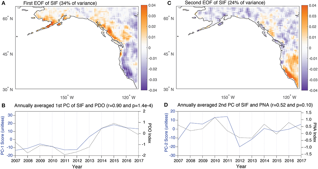
Figure 3. (A,C) The first and second EOF of SIF for the region of interest. The units are dimensionless loadings with explained variances of 34 and 24%, respectively. (B,D) The first and second annually averaged vectors of the PCs associated with the EOFs shown in above panels. The first PC vector is plotted alongside the annually-averaged PDO index (r = 0.90) and the second PC is plotted alongside PNA (r = 0.52).
The EOF analysis of chlorophyll is also characterized by two dominant modes of variability that similarly explain 33 and 25% of the variance. With both modes, the dominant loading centers occur along the coastlines where the majority of variance occurs. The first of the EOF patterns is characterized by a strong dipole with negative loadings along the central and southern California coastline and south of the Aleutian Islands. This mode is associated with positive anomalies that span the coast of northern California, Oregon, British Columbia and through to southern Alaska (Figure 4A). The PC of this EOF strongly correlates with ENSO (r = 0.85) (Figure 4B). The influence of ENSO on coastal chlorophyll is through the combined effects of changes in the tropical Pacific thermocline that migrate poleward and changes in coastal winds associated with the establishment and strength of atmospheric blocking cells in the North Pacific (Jacox et al., 2015). The second EOF of chlorophyll is associated with a widespread but diffuse negative loading along the entire coastline with isolated positive loading anomalies along the Northern California and Oregon coastlines and Vancouver Island (Figure 4C). This mode is associated with more low frequency variance and correlates most strongly with the PDO (r = 0.69) (Figure 4D) (Chhak and Di Lorenzo, 2007).
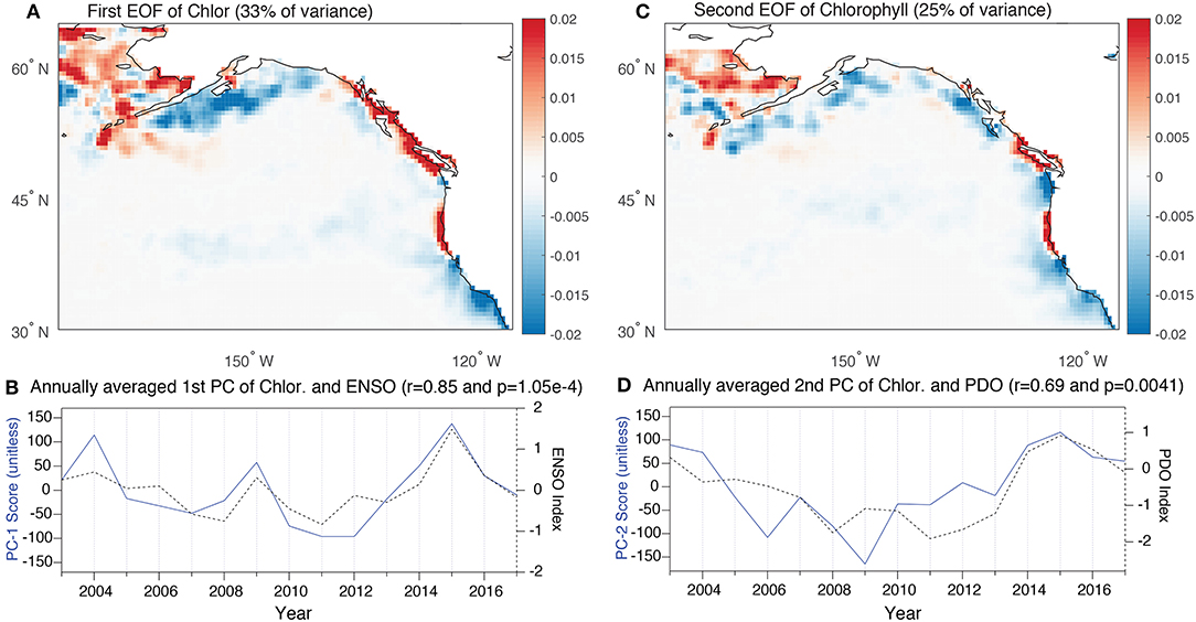
Figure 4. (A,C) The first and second EOF of chlorophyll for the region of interest. The units are dimensionless loadings with explained variances of 33 and 25%, respectively. (B,D) The first and second annually averaged vectors of the PCs associated with the EOFs shown in above panels. The first PC is plotted alongside the annually-averaged ENSO index (r = 0.89) and the second PC is plotted alongside PDO as in Figure 2 (r = 0.69).
By combining the normalized maps of SIF and chlorophyll, a third EOF analysis was done to specifically assess whether the basin-wide mode of productivity generates coherent loading between adjacent coastal and terrestrial regions. The first EOF of this field explains 33% of the variance (Figure 5A) and is associated with a strong dipole pattern centered at ~40°N. While the EOFs of individual SIF and chlorophyll fields implied there would be shared spatial variance associated with the PDO, this analysis provides explicit evidence of variability that is seamless across the marine and terrestrial interface over broad regions of the coastline from California to southern Alaska. The aquatic-terrestrial synchrony exists because of the presence of a “mirrored dipole” such that both the marine and terrestrial systems display dipoles with similar spatial extents and loadings in the same direction. The PC associated with the mirrored dipole EOF is strongly correlated with the PDO (r = 0.89) (Figure 5B). The evidence for strong synchrony in California is consistent with previous results from Black et al. (2018) but has been expanded here across a larger domain. Only a single EOF is shown for the joint marine/terrestrial field because all subsequent modes had limited explanatory power.
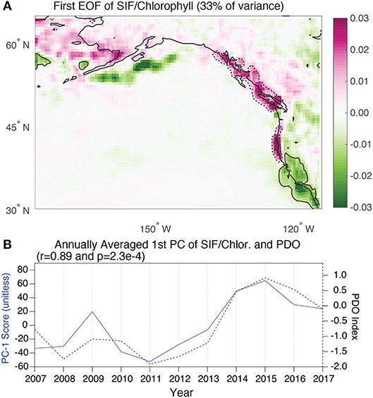
Figure 5. (A) The first EOF of the merged normalized SIF and chlorophyll maps for the region of interest. The units are dimensionless loadings with an explained variance of 33%. The dark contour (dotted and continuous) are used to highlight particular areas of synchrony and asynchrony, respectively. (B) The first annually-averaged PC vector associated with the EOF shown in above panel. The PC timeseries is plotted alongside the annually-averaged PDO index (r = 0.89).
3.3. Case Studies of 2009, 2012 and 2015
To complement the EOF analyses, a specific assessment of the absolute chlorophyll and SIF anomalies during selected years was conducted. The first of these years, 2015, was chosen as one where SIF (Figure 3), chlorophyll (Figure 4) and the joint SIF/chlorophyll (Figure 5) EOF analyses all indicated a strong north-south dipole pattern. The pattern of SIF and chlorophyll anomalies during 2015 (Figure 6A), were characterized by significant negative anomalies in productivity along the California coastline and positive anomalies across much of coastal British Columbia and southern Alaska. The dipole pattern in both terrestrial and marine productivity thus produce widespread synchrony. It is noted, however, that further north into Alaska the synchrony breaks down such that the terrestrial ecosystems were associated with positive anomalies and the ocean with negative anomalies. In contrast to 2015, 2012 was a year that was associated with a negative loading in the PC score of the joint SIF/Chlorophyll EOF (Figure 5). Indeed, unlike 2015, 2012 was not associated with a chlorophyll dipole but rather a widespread negative loading across the coastline from California through to southern Alaska. This pattern was largely mirrored on land with relatively low SIF values across the region. Like 2015, 2012 was thus also associated with synchronous behavior but with a pattern distinct from the familiar dipole. The last year considered was 2009, which was chosen as a contrasting example, where the first PC of chlorophyll indicated a strongly positive anomaly whereas the first PC of SIF indicated a weak or inverted anomaly pattern. Indeed, 2009 was associated with strongly opposing anomalies between productivity in the land and sea across much of the California coastline and northward to southern Alaska (Figure 6B). The conditions during 2009 represent the only year in the timeseries with significantly asynchronous behavior.
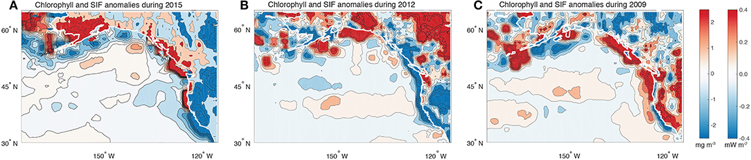
Figure 6. Maps showing the annually-averaged anomalies in SIF and chlorophyll during the 2015 (A), 2012 (B), and 2009 (C) calendar years.
To explain the distinct pattern between years, we begin with an analysis of the annually averaged climate modes for these years. 2015 was associated with both strong ENSO and PDO anomalies, with the former driving the dipole pattern in chlorophyll and the latter the dipole pattern in SIF (Fisher et al., 2015; Lindegren et al., 2018) (Figures 3, 4). In contrast, 2009 was associated with a negative PDO and positive ENSO, such that the terrestrial dipole was inverted relative to 2015 and the chlorophyll dipole remained the same. The effect was strong terrestrial-marine asynchrony during this year. The comparison between these years suggests that when ENSO and PDO are in phase, synchrony emerges and when the two are out of phase asynchrony emerges. However, the year of 2012 challenges this simple depiction as this year had similar annual averages for both ENSO and the PDO as 2009 yet also exhibited synchrony. It is likely that the difference between 2009 and 2012 emerged because of subseasonal variations in ENSO and the PDO. Specifically, in 2009 ENSO began negative but transitioned to a positive state. In contrast, 2012 ENSO and PDO were persistently out of phase throughout the year.
To further explore the mechanisms associated with synchrony (2015) or asynchrony (2009), a comparison between the climate conditions of these two contrasting years was conducted. During the winter, 2015 had a significantly stronger and southerly displaced Aleutian Low relative to 2009. This led to enhanced southerly winds during the winter months (Wise, 2016) (Figure 7A). The wintertime atmospheric conditions may have preconditioned growing season productivity anomalies through changes in snowpack and soil moisture. Specifically, this atmospheric pattern would have lead to storm tracks focused along the British Columbian coastline and southern Alaska (Ropelewski and Halpert, 1986; McCabe et al., 2004). It is also notable that 2015 was associated with anomalously warm (cool) conditions in the spring and early summer in the northern (southern) regions of the domain along with anomalous northerly winds across the coastlines north of California (Smith and Sardeshmukh, 2000) (Figure 7B). These patterns would have contributed to an earlier onset of spring in the north and the positive anomalies in SIF (McCabe et al., 2012). The coastal wind field anomalies along the British Columbian and southern Alaskan coastlines would also have lead to increased upwelling or reduced downwelling and contributed to the observed positive chlorophyll anomalies. The comparison between 2009 and 2015 reveals effects during both winter and summer months and highlights why the use of annual averages for the climate modes produced the strongest correlations with the EOF patterns.
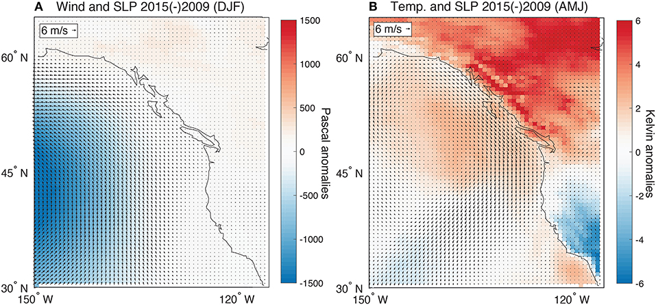
Figure 7. (A) The difference in SLP and 10 m wind fields for DJF between 2015 and 2009. Units for SLP are Pa and the wind vectors are plotted with reference to 6 m s−1 vector shown in the top left. (B) The 2 m air temperature and 10 m wind fields for AMJ between 2015 and 2009. Units for temperature are K and the wind vectors are plotted with reference to 6 m s−1 vector shown in the top left. All data were extracted from the MERRA reanalysis database (Rienecker et al., 2011).
3.4. Spatial Analysis of Synchrony From Regression Analysis
Figure 8 shows the correlation coefficient between adjacent marine and terrestrial domains along the entire coastline. The results show that along ~40% of the coastline there is a statistically significant interannual correlation between SIF and chlorophyll. The correlation is strongest at the Southern California Bight, along the Oregon and Vancouver Island coastlines and along the southern Alaskan coast (Figure 8A). While there are a few regions of the coast where the correlation is negative (i.e., asynchrony), the principal pattern is one of synchrony. This shows that in spite of the complexities of the spatiotemporal aspects of synchrony, as described in the previous analyses, coastal regions broadly exhibit terrestrial-marine synchrony. Alongside the correlation map, is a separate analysis showing the lag between when terrestrial and aquatic ecosystems experience their respective peaks in productivity (Figure 8B). A comparison between these maps shows that synchrony, or lack thereof, is not tied in any systematic way to local differences between terrestrial and marine seasonality. This can be explained by the fact that the processes driving annual variations in productivity, whether it be marine or terrestrial, persist for multiple months.
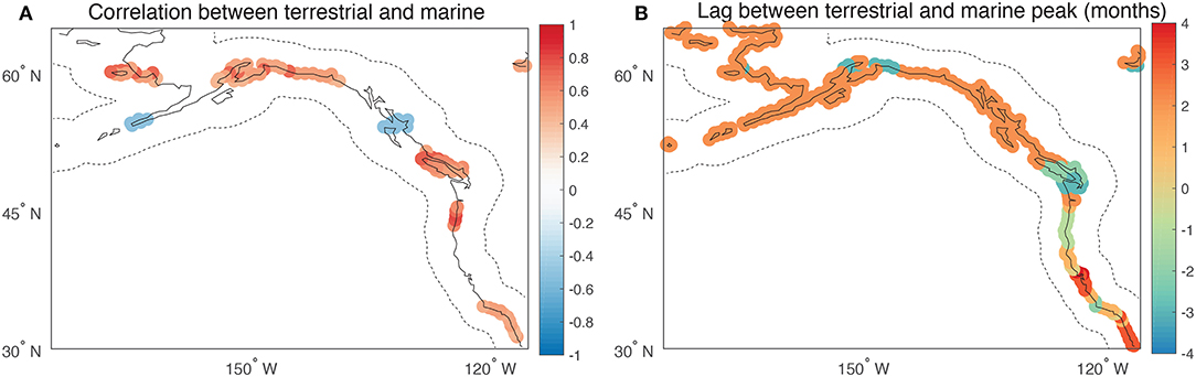
Figure 8. (A) Map showing the correlation coefficient between adjacent (± 300 km as contained by the dotted lines) swaths of land (SIF) and sea (chlorophyll). Points are only plotted where the p-value of the correlation is <0.1. (B) The lag between when adjacent land and sea regions reach their peak in productivity with units of month. The scale of regions used in the calculation are identical to those used in (A). The calculation of when the peak in productivity occurred is as shown in Figure 2.
4. Discussion
The analyses presented here were designed to test whether synchrony between terrestrial and marine ecosystems is a fundamental characteristic of the North Pacific. Previous work along the California coastline established the presence of regional-scale coherence that manifested at the scale of species (Black et al., 2018). This previous work hypothesized that the mechanism linking ecosystems across the coastal interface was atmospheric circulation anomalies that simultaneously influenced upwelling through altered wind fields and rainfall through variations in the storm track. However, across 1000's of km of coastline the large scale coupling associated with atmospheric modes could be strengthened or weakened through myriad secondary mechanisms operating at the local scale. These could include the influence of SSTs on the development of marine fog, the effect of SSTs on convective storm development and atmospheric humidity and changes in runoff that influence marine productivity through nutrient availability (Persson et al., 2005; Warrick et al., 2005; Johnstone and Dawson, 2010). In considering the diverse ways that marine and terrestrial ecosystems could become coupled through climate variability, it is feasible that the synchrony previously observed at the regional scale may only emerge under a specific set of conditions.
As illustrated by the EOF analyses of SIF and chlorophyll (Figures 3, 4), productivity is characterized in both the marine and terrestrial ecosystems by north-south dipole modes that correlate strongly with known ocean-atmosphere indices (Hare and Mantua, 2000; Di Lorenzo et al., 2008). ENSO is the dominant driver for the chlorophyll variability with strong localized and opposing loading centers that reflect the response of upwelling to wind and thermocline anomalies (Karl et al., 1995; Jacox et al., 2015; García-Reyes et al., 2018). Surprisingly, the EOF analysis of SIF did not indicate any strong impact of ENSO on the dominant spatiotemporal patterns in terrestrial ecosystems (Cayan et al., 1999; McCabe et al., 2012). It may be that because the effects of ENSO are strongest in the semi-arid water-limited regions in the southwestern US, the apparent effect of ENSO was minimized by including northern latitudes in the analysis. Instead, the results showed that terrestrial productivity was predominately driven by lower frequency (multi-annual) variability, which is in phase with the PDO (MacDonald and Case, 2005; Fang et al., 2018). The dominant influence of PDO on the spatiotemporal pattern reflects not only precipitation changes associated with this oceanic mode of variability but also through its effects on surface temperatures in coastal British Columbia and southern Alaska (Steinman et al., 2014).
Despite the fact that the leading terrestrial and marine EOFs were correlated with different ocean-atmospheric modes, the combined EOF analysis showed strong evidence that the PDO can generate a mirrored dipole pattern with coherent terrestrial and marine anomalies that span 1000's of km of the North Pacific coastline (Figure 5). That said, regions of isolated asynchrony associated with this dominant mode of variability were present along the Washington coastline and off the Aleutian Islands. The isolated areas of asynchrony highlight where local processes acting on either the marine or terrestrial systems may disrupt the joint sensitivity of terrestrial and marine ecosystems to ocean-atmosphere variability. When considering this result along with the regression analysis presented in Figure 8, it can be concluded that synchrony is a widespread phenomenon along the eastern margin of the North Pacific. This is apparently the case even when distinct ENSO and PDO states prevail as illustrated by synchrony during 2012 and 2015 despite differences in ENSO and PDO states. One potential factor considered here to explain the spatial pattern of synchrony was the seasonal phasing between adjacent terrestrial and marine systems. It was presumed a priori that in areas where the seasonal cycles of land and sea productivity were in phase, there would be greater synchrony. However, there was limited evidence to suggest this was the case (Figure 8), implying that synchrony does not generally emerge in this region from the immediate responses to specific synoptic events such as a heatwave or flood states (Ruthrof et al., 2018). Instead, the results suggest that synchrony reflects more slowly evolving responses to preceding wintertime atmospheric circulation patterns and springtime temperatures. The consequence is that even in areas where the terrestrial and aquatic ecosystems lag one another by 3–4 months, there may still be interannual coherence.
The examples of 2009 and 2015 highlight how ENSO and PDO modes can modulate the strength of synchrony. Although the analysis is based on only a short timeseries, the results suggest that simultaneously positive ENSO and PDO modes drive synchrony (2015) while positive ENSO and negative PDO lead to asynchrony (2009). The analysis relied on annual averages of these two modes, which is in contrast to previous studies that tended to focus on wintertime values when these patterns manifest most strongly. Future studies would benefit from exploring in more detail how specific seasonal patterns might strengthen or disrupt synchrony. Nonetheless, to the extent that PDO and ENSO can become phase locked for multiple years (or longer) (Newman et al., 2003), synchrony would be the dominant pattern over longer time periods. This is relevant in considering proxy records where it can be expected that the correlation between proxies for land and sea productivity (such as tree growth and δ13C of foraminifera) would predominantly reflect variations in the PDO or a similar mode of variability. The exact physical mechanism that drives synchrony during positive PDO and ENSO cannot be ascertained without further modeling but the analysis of climate conditions during opposing years suggests it emerges from a combination of: (1) a strong Aleutian Low that drives anomalous wintertime southerly winds, (2) a dipole in spring temperature anomalies over land that impact growing season length and (3) anomalous northerly coastal wind fields that influence coastal upwelling or downwelling. A longer timeseries that includes additional examples of joint ENSO and PDO anomalies, including ones with specific seasonal manifestations, would help to further shed light on the dynamics that underlie the synchrony.
The broader motivation in quantifying synchrony was to assess whether coupling between terrestrial and marine productivity would amplify the sensitivity of the global carbon cycle to interannual climate variability. Existing data suggest that the strength of the ocean and terrestrial carbon sinks are important sources of interannual variability of the carbon budget (Ballantyne et al., 2012). Despite the extensive work done on this topic, few studies have addressed whether the terrestrial and marine carbon sinks become synchronized in response to ocean-atmosphere climate modes. The results from this study show that the terrestrial and marine carbon sinks in the western US are highly responsive to climate variability, which is consistent with previous assessments on the role of semi-arid and mid-latitude ecosystems on interannual variability of the global carbon cycle (Poulter et al., 2014; Ahlström et al., 2015; Berkelhammer et al., 2017). However, both terrestrial and aquatic systems respond to interannual modes with a north-south dipole such that the total regional carbon sink (i.e., integrated anomalies across the domain) is not likely to show significant interannual changes. However, there will be latitudinal shifts in where primary productivity is highest and also locations such as the California and British Columbian coasts that are associated with locally enhanced (or diminished) carbon sinks that result from the mirrored terrestrial and marine dipole.
An important caveat to this study is that while chlorophyll and SIF provide indicators of changes in productivity, they do not provide constraints on the net ecosystem exchange of carbon (i.e., respiration-photosynthesis). This is specifically an issue with chlorophyll, which is an indicator of biomass concentration but not directly for primary productivity. Further, the marine flux of carbon is tightly controlled by physical processes, which may be more important to air-sea exchange of carbon than primary productivity (Eddebbar et al., 2017). To fully assess whether terrestrial and marine synchrony influences regional carbon budgets, a more holistic approach is needed that considers both the physical aspects of air-sea exchange of carbon and how terrestrial respiration is also responding to climate variability (Li et al., 2016; Liu et al., 2017). Ultimately, whether terrestrial and marine synchrony play an important role in interannual carbon budgets will depend on whether the behavior observed here in the North Pacific is common elsewhere. Future studies on this topic might find additionally strong examples of synchrony in regions such as southern South America and the high Arctic where the seasonality of terrestrial and aquatic productivity are in phase with one another (not shown). The data are available to test this and as new satellite platforms generate data with higher spatial resolution and accuracy, a better understanding of the importance of these linkages will be possible.
5. Conclusions
This study set out to test whether the productivity of terrestrial and marine ecosystems in the North Pacific display synchronous responses to climate variability. Previous work had addressed this topic in the context of trophic dynamics but we consider here whether this synchrony may enhance the response of regional carbon cycle dynamics to climate variability. The results show that over 1,000's of km of the North Pacific coastline, there is a common temporal response between the productivity of adjacent terrestrial and marine ecosystems. While there are exceptions to this behavior, the results suggest that the effects of ocean-atmosphere variability on wind fields, rainfall and temperature have a tendency to produce common or synchronous responses across the coastal interface. The synchrony appears most pronounced in response to the Pacific Decadal Oscillation (PDO) though this is apparently modulated by the state of ENSO, such that if ENSO and the PDO oppose one another so too does the strength of coupling between terrestrial and marine productivity. The results ultimately suggest there is not likely to be a significant region-wide response of the carbon cycle to this synchrony because the modes of variability are predominated by opposing north-south anomalies such that there are rarely examples of basin-scale productivity anomalies as in 2012. However, there may be local regions such as the California coastline where the synchrony is strong enough to influence the regional carbon sink. Future studies using Earth System Models that include both the terrestrial and marine carbon cycles could be used to explore the dynamics that give rise to the regions of highly synchronous behavior particularly in the context of canonical ENSO and PDO climate variability.
Author Contributions
MB designed the research, performed all the analyses and wrote the paper.
Funding
Funding for this research was provided by NSF grant #1502776 to MB.
Conflict of Interest Statement
The author declares that the research was conducted in the absence of any commercial or financial relationships that could be construed as a potential conflict of interest.
Acknowledgments
The author would like to thank J. Joiner and the rest of the MetOp team for making the fluorescence data available.
References
Abram, N. J., McGregor, H. V., Tierney, J. E., Evans, M. N., McKay, N. P., Kaufman, D. S., et al. (2016). Early onset of industrial-era warming across the oceans and continents. Nature 536, 411. doi: 10.1038/nature19082
Ahlström, A., Raupach, M. R., Schurgers, G., Smith, B., Arneth, A., Jung, M., et al. (2015). The dominant role of semi-arid ecosystems in the trend and variability of the land CO2 sink. Science 348, 895–899. doi: 10.1126/science.aaa1668
Ahmed, M., Anchukaitis, K. J., Asrat, A., Borgaonkar, H. P., Braida, M., Buckley, B. M., et al. (2013). Continental-scale temperature variability during the past two millennia. Nat. Geosci. 6, 339. doi: 10.1038/ngeo1797
Ballantyne, A., Alden, C., Miller, J., Tans, P., and White, J. (2012). Increase in observed net carbon dioxide uptake by land and oceans during the past 50 years. Nature 487, 70. doi: 10.1038/nature11299
Behrenfeld, M. J., O'Malley, R. T., Siegel, D. A., McClain, C. R., Sarmiento, J. L., Feldman, G. C., et al. (2006). Climate-driven trends in contemporary ocean productivity. Nature 444, 752. doi: 10.1038/nature05317
Berkelhammer, M., Stefanescu, I., Joiner, J., and Anderson, L. (2017). High sensitivity of gross primary production in the Rocky Mountains to summer rain. Geophys. Res. Lett. 44, 3643–3652. doi: 10.1002/2016GL072495
Biondi, F., Gershunov, A., and Cayan, D. R. (2001). North pacific decadal climate variability since 1661. J. Clim. 14, 5–10. doi: 10.1175/1520-0442(2001)014<0005:NPDCVS>2.0.CO;2
Björnsson, H., and Venegas, S. (1997). A manual for eof and svd analyses of climatic data. CCGCR Rep. 97, 112–134.
Black, B. A., Sydeman, W. J., Frank, D. C., Griffin, D., Stahle, D. W., García-Reyes, M., et al. (2014). Six centuries of variability and extremes in a coupled marine-terrestrial ecosystem. Science 345, 1498–1502. doi: 10.1126/science.1253209
Black, B. A., van der Sleen, P., Di Lorenzo, E., Griffin, D., Sydeman, W. J., Dunham, J. B., et al. (2018). Rising synchrony controls western North American ecosystems. Glob. Change Biol. 24, 2305–2314. doi: 10.1111/gcb.14128
Cayan, D. R., Redmond, K. T., and Riddle, L. G. (1999). ENSO and hydrologic extremes in the western United States. J. Clim. 12, 2881–2893. doi: 10.1175/1520-0442(1999)012<2881:EAHEIT>2.0.CO;2
Chhak, K., and Di Lorenzo, E. (2007). Decadal variations in the California Current upwelling cells. Geophys. Res. Lett. 34:L14604. doi: 10.1029/2007GL030203
Cook, E. R., Seager, R., Cane, M. A., and Stahle, D. W. (2007). North American drought: Reconstructions, causes, and consequences. Earth Sci. Rev. 81, 93–134. doi: 10.1016/j.earscirev.2006.12.002
Di Lorenzo, E., Schneider, N., Cobb, K. M., Franks, P., Chhak, K., Miller, A. J., et al. (2008). North Pacific Gyre Oscillation links ocean climate and ecosystem change. Geophys. Res. Lett. 35. doi: 10.1029/2007GL032838
Dore, J. E., Letelier, R. M., Church, M. J., Lukas, R., and Karl, D. M. (2008). Summer phytoplankton blooms in the oligotrophic North Pacific Subtropical Gyre: historical perspective and recent observations. Progr. Oceanogr. 76, 2–38. doi: 10.1016/j.pocean.2007.10.002
Eddebbar, Y. A., Long, M. C., Resplandy, L., Rödenbeck, C., Rodgers, K. B., Manizza, M., et al. (2017). Impacts of ENSO on air-sea oxygen exchange: observations and mechanisms. Glob. Biogeochem. Cycles 31, 901–921. doi: 10.1002/2017GB005630
Fang, K., Cook, E., Guo, Z., Chen, D., Ou, T., and Zhao, Y. (2018). Synchronous multi-decadal climate variability of the whole Pacific areas revealed in tree rings since 1567. Environ. Res. Lett. 13, 024016. doi: 10.1088/1748-9326/aa9f74
Fisher, J. L., Peterson, W. T., and Rykaczewski, R. R. (2015). The impact of E l N iño events on the pelagic food chain in the northern California Current. Glob. Change Biol. 21, 4401–4414. doi: 10.1111/gcb.13054
García-Reyes, M., Lamont, T., Sydeman, W. J., Black, B. A., Rykaczewski, R. R., Thompson, S. A., et al. (2018). A comparison of modes of upwelling-favorable wind variability in the Benguela and California current ecosystems. J. Mar. Syst. 188, 17–26. doi: 10.1016/j.jmarsys.2017.06.002
Guyette, R. P., and Rabeni, C. F. (1995). Climate response among growth increments of fish and trees. Oecologia 104, 272–279. doi: 10.1007/BF00328361
Hare, S. R., and Mantua, N. J. (2000). Empirical evidence for North Pacific regime shifts in 1977 and 1989. Progr. Oceanogr. 47, 103–145. doi: 10.1016/S0079-6611(00)00033-1
Hilton, T. W., Whelan, M. E., Zumkehr, A., Kulkarni, S., Berry, J. A., Baker, I. T., et al. (2017). Peak growing season gross uptake of carbon in north america is largest in the midwest usa. Nat. Clim. Change 7, 450–454. doi: 10.1038/nclimate3272
Hoegh-Guldberg, O., and Bruno, J. F. (2010). The impact of climate change on the world's marine ecosystems. Science 328, 1523–1528. doi: 10.1126/science.1189930
Hu, C., Lee, Z., and Franz, B. (2012). Chlorophyll aalgorithms for oligotrophic oceans: a novel approach based on three-band reflectance difference. J. Geophys. Res. 117. doi: 10.1029/2011JC007395
Hurlburt, H. E., Wallcraft, A. J., Schmitz, W. J., Hogan, P. J., and Metzger, E. J. (1996). Dynamics of the Kuroshio/Oyashio current system using eddy-resolving models of the North Pacific Ocean. J. Geophys. Res. 101, 941–976. doi: 10.1029/95JC01674
Jacox, M. G., Fiechter, J., Moore, A. M., and Edwards, C. A. (2015). ENSO and the california current coastal upwelling response. J. Geophys. Res. 120, 1691–1702. doi: 10.1002/2014JC010650
Jeong, S.-J., Schimel, D., Frankenberg, C., Drewry, D. T., Fisher, J. B., Verma, M., et al. (2017). Application of satellite solar-induced chlorophyll fluorescence to understanding large-scale variations in vegetation phenology and function over northern high latitude forests. Remote Sens. Environ. 190, 178–187. doi: 10.1016/j.rse.2016.11.021
Johnstone, J. A., and Dawson, T. E. (2010). Climatic context and ecological implications of summer fog decline in the coast redwood region. Proc. Natl. Acad. Sci. U.S.A. 107, 4533–4538. doi: 10.1073/pnas.0915062107
Joiner, J., Guanter, L., Lindstrot, R., Voigt, M., Vasilkov, A., Middleton, E., et al. (2013). Global monitoring of terrestrial chlorophyll fluorescence from moderate spectral resolution near-infrared satellite measurements: methodology, simulations, and application to gome-2. Atmos. Meas. Techn. 6, 2803–2823. doi: 10.5194/amt-6-2803-2013
Joiner, J., Yoshida, Y., Vasilkov, A., Schaefer, K., Jung, M., Guanter, L., et al. (2014). The seasonal cycle of satellite chlorophyll fluorescence observations and its relationship to vegetation phenology and ecosystem atmosphere carbon exchange. Remote Sens. Environ. 152, 375–391. doi: 10.1016/j.rse.2014.06.022
Karl, D., Letelier, R., Hebel, D., Tupas, L., Dore, J., Christian, J., et al. (1995). Ecosystem changes in the North Pacific subtropical gyre attributed to the 1991–92 El Nino. Nature 373, 230. doi: 10.1038/373230a0
Landschuetzer, P., Gruber, N., and Bakker, D. C. (2016). Decadal variations and trends of the global ocean carbon sink. Glob. Biogeochem. Cycles 30, 1396–1417. doi: 10.1002/2015GB005359
Le Quéré, C., Andres, R. J., Boden, T., Conway, T., Houghton, R. A., House, J. I., et al. (2012). The global carbon budget 1959–2011. Earth Syst. Sci. Data Discuss. 5, 1107–1157. doi: 10.5194/essdd-5-1107-2012
Leathers, D. J., Yarnal, B., and Palecki, M. A. (1991). The Pacific/North American teleconnection pattern and United States climate. Part I: regional temperature and precipitation associations. J. Clim. 4, 517–528. doi: 10.1175/1520-0442(1991)004<0517:TPATPA>2.0.CO;2
Li, W., Ciais, P., Wang, Y., Peng, S., Broquet, G., Ballantyne, A. P., et al. (2016). Reducing uncertainties in decadal variability of the global carbon budget with multiple datasets. Proc. Natl. Acad. Sci. U.S.A. 13, 13104–13108. doi: 10.1073/pnas.1603956113
Lindegren, M., Checkley, D. M. Jr., Koslow, J. A., Goericke, R., and Ohman, M. D. (2018). Climate-mediated changes in marine ecosystem regulation during El Niño. Glob. Change Biol. 24, 796–809. doi: 10.1111/gcb.13993
Liu, J., Bowman, K. W., Schimel, D. S., Parazoo, N. C., Jiang, Z., Lee, M., et al. (2017). Contrasting carbon cycle responses of the tropical continents to the 2015–2016 El Niño. Science 358:eaam5690. doi: 10.1126/science.aam5690
Luus, K., Commane, R., Parazoo, N., Benmergui, J., Euskirchen, E., Frankenberg, C., et al. (2017). Tundra photosynthesis captured by satellite-observed solar-induced chlorophyll fluorescence. Geophys. Res. Lett. 44, 1564–1573. doi: 10.1002/2016GL070842
MacDonald, G. M., and Case, R. A. (2005). Variations in the Pacific Decadal Oscillation over the past millennium. Geophys. Res. Lett. 32. doi: 10.1029/2005GL022478
Mantua, N. J., and Hare, S. R. (2002). The Pacific Decadal Oscillation. J. Oceanogr. 58, 35–44. doi: 10.1023/A:1015820616384
Mantua, N. J., Hare, S. R., Zhang, Y., Wallace, J. M., and Francis, R. C. (1997). A Pacific interdecadal climate oscillation with impacts on salmon production. Bull. Am. Meteorol. Soc. 78, 1069–1080. doi: 10.1175/1520-0477(1997)078<1069:APICOW>2.0.CO;2
McCabe, G. J., Ault, T. R., Cook, B. I., Betancourt, J. L., and Schwartz, M. D. (2012). Influences of the El Niño Southern Oscillation and the Pacific Decadal Oscillation on the timing of the North American spring. Int. J. Climatol. 32, 2301–2310. doi: 10.1002/joc.3400
McCabe, G. J., Palecki, M. A., and Betancourt, J. L. (2004). Pacific and Atlantic Ocean influences on multidecadal drought frequency in the United States. Proc. Natl. Acad. Sci. U.S.A. 101, 4136–4141. doi: 10.1073/pnas.0306738101
Messié, M., and Chavez, F. (2011). Global modes of sea surface temperature variability in relation to regional climate indices. J. Clim. 24, 4314–4331. doi: 10.1175/2011JCLI3941.1
Newman, M., Compo, G. P., and Alexander, M. A. (2003). ENSO-forced variability of the Pacific decadal oscillation. J. Clim. 16, 3853–3857. doi: 10.1175/1520-0442(2003)016<3853:EVOTPD>2.0.CO;2
Ong, J. J., Rountrey, A. N., Zinke, J., Meeuwig, J. J., Grierson, P. F., O'donnell, A. J., et al. (2016). Evidence for climate-driven synchrony of marine and terrestrial ecosystems in northwest Australia. Glob. Change Biol. 22, 2776–2786. doi: 10.1111/gcb.13239
Persson, P. O. G., Neiman, P., Walter, B., Bao, J., and Ralph, F. (2005). Contributions from California coastal-zone surface fluxes to heavy coastal precipitation: a CALJET case study during the strong El Niño of 1998. Mon. Weather Rev. 133, 1175–1198. doi: 10.1175/MWR2910.1
Platt, T., Caverhill, C., and Sathyendranath, S. (1991). Basin-scale estimates of oceanic primary production by remote sensing: the North Atlantic. J. Geophys. Res. 96, 15147–15159. doi: 10.1029/91JC01118
Poulter, B., Frank, D., Ciais, P., Myneni, R. B., Andela, N., Bi, J., et al. (2014). Contribution of semi-arid ecosystems to interannual variability of the global carbon cycle. Nature 509, 600. doi: 10.1038/nature13376
Rienecker, M. M., Suarez, M. J., Gelaro, R., Todling, R., Bacmeister, J., Liu, E., et al. (2011). MERRA: NASA's modern-era retrospective analysis for research and applications. J. Clim. 24, 3624–3648. doi: 10.1175/JCLI-D-11-00015.1
Ropelewski, C. F., and Halpert, M. S. (1986). North American precipitation and temperature patterns associated with the El Niño/Southern Oscillation (ENSO). Mon. Weather Rev. 114, 2352–2362. doi: 10.1175/1520-0493(1986)114<2352:NAPATP>2.0.CO;2
Rosenzweig, C., Karoly, D., Vicarelli, M., Neofotis, P., Wu, Q., Casassa, G., et al. (2008). Attributing physical and biological impacts to anthropogenic climate change. Nature 453, 353. doi: 10.1038/nature06937
Ruthrof, K. X., Breshears, D. D., Fontaine, J. B., Froend, R. H., Matusick, G., Kala, J., et al. (2018). Subcontinental heat wave triggers terrestrial and marine, multi-taxa responses. Sci. Rep. 8, 13094. doi: 10.1038/s41598-018-31236-5
Salathé, E. P. Jr. (2006). Influences of a shift in North Pacific storm tracks on western North American precipitation under global warming. Geophys. Res. Lett. 33:L19820. doi: 10.1029/2006GL026882
Smith, C. A., and Sardeshmukh, P. D. (2000). The effect of ENSO on the intraseasonal variance of surface temperatures in winter. Int. J. Climatol. 20, 1543–1557. doi: 10.1002/1097-0088(20001115)20:13<1543::AID-JOC579>3.0.CO;2-A
Steinman, B. A., Abbott, M. B., Mann, M. E., Ortiz, J. D., Feng, S., Pompeani, D. P., et al. (2014). Ocean-atmosphere forcing of centennial hydroclimate variability in the Pacific Northwest. Geophys. Res. Lett. 41, 2553–2560. doi: 10.1002/2014GL059499
St. George, S., Meko, D. M., and Cook, E. R. (2010). The seasonality of precipitation signals embedded within the North American Drought Atlas. Holocene 20, 983–988. doi: 10.1177/0959683610365937
Trouet, V., and Taylor, A. H. (2010). Multi-century variability in the Pacific North American circulation pattern reconstructed from tree rings. Clim. Dyn. 35, 953–963. doi: 10.1007/s00382-009-0605-9
Warrick, J. A., Washburn, L., Brzezinski, M. A., and Siegel, D. A. (2005). Nutrient contributions to the Santa Barbara Channel, California, from the ephemeral Santa Clara River. Estuarine Coastal Shelf Sci. 62, 559–574. doi: 10.1016/j.ecss.2004.09.033
Wise, E. K. (2016). Five centuries of US West Coast drought: Occurrence, spatial distribution, and associated atmospheric circulation patterns. Geophys. Res. Lett. 43, 4539–4546. doi: 10.1002/2016GL068487
Keywords: climate, ecohydrology, carbon cycle, remote sensing, fluorescence
Citation: Berkelhammer M (2019) Synchronous Modes of Terrestrial and Marine Productivity in the North Pacific. Front. Earth Sci. 7:73. doi: 10.3389/feart.2019.00073
Received: 06 November 2018; Accepted: 22 March 2019;
Published: 16 April 2019.
Edited by:
Miriam Jones, United States Geological Survey, United StatesReviewed by:
Milad Janalipour, K. N. Toosi University of Technology, IranAndrew C. Thomas, University of Maine, United States
Copyright © 2019 Berkelhammer. This is an open-access article distributed under the terms of the Creative Commons Attribution License (CC BY). The use, distribution or reproduction in other forums is permitted, provided the original author(s) and the copyright owner(s) are credited and that the original publication in this journal is cited, in accordance with accepted academic practice. No use, distribution or reproduction is permitted which does not comply with these terms.
*Correspondence: Max Berkelhammer, YmVya2VsaGFAdWljLmVkdQ==