Holocene Thermokarst Lake Dynamics in Northern Interior Alaska: The Interplay of Climate, Fire, and Subsurface Hydrology

Anderson, Lesleigh; Edwards, Mary; Shapley, Mark D.; Finney, Bruce P.; Langdon, Catherine

doi:10.3389/feart.2019.00053

ORIGINAL RESEARCH article

Front. Earth Sci., 03 April 2019

Sec. Quaternary Science, Geomorphology and Paleoenvironment

Volume 7 - 2019 | https://doi.org/10.3389/feart.2019.00053

This article is part of the Research Topic North Pacific Environment and Paleoclimate from the Late Pleistocene to Present View all 13 articles

Holocene Thermokarst Lake Dynamics in Northern Interior Alaska: The Interplay of Climate, Fire, and Subsurface Hydrology

$\r\nLesleigh Anderson*$ Lesleigh Anderson^1*

Mary Edwards²

Mark D. Shapley³

Bruce P. Finney^4,5

Catherine Langdon²

¹U.S. Geological Survey, Geosciences and Environmental Change Science Center, Denver, CO, United States
²School of Geography and Environment, University of Southampton, Highfield, United Kingdom
³Continental Scientific Drilling Coordination Office and National Lacustrine Core Facility (LacCore), University of Minnesota, Minneapolis, MN, United States
⁴Department of Biological Sciences, Idaho State University, Pocatello, ID, United States
⁵Department of Geosciences, Idaho State University, Pocatello, ID, United States

The current state of permafrost in Alaska and meaningful expectations for its future evolution are informed by long-term perspectives on previous permafrost degradation. Thermokarst processes in permafrost landscapes often lead to widespread lake formation and the spatial and temporal evolution of thermokarst lake landscapes reflects the combined effects of climate, ground conditions, vegetation, and fire. This study provides detailed analyses of thermokarst lake sediments of Holocene age from the southern loess uplands of the Yukon Flats, including bathymetry and sediment core analyses across a water depth transect. The sediment core results, dated by radiocarbon and ²¹⁰Pb, indicate the permanent onset of finely laminated lacustrine sedimentation by ∼8,000 cal yr BP, which followed basin development through inferred thermokarst processes. Thermokarst expansion to modern shoreline configurations continued until ∼5000 cal yr BP and may have been influenced by increased fire. Between ∼5000 and 2000 cal yr BP, the preservation of fine laminations at intermediate and deep-water depths indicate higher lake levels than present. At that time, the lake likely overflowed into an over-deepened gully system that is no longer occupied by perennial streams. By ∼2000 cal yr BP, a shift to massive sedimentation at intermediate water depths indicates that lake levels lowered, which is interpreted to reflect a response to drier conditions based on correspondence with Yukon Flats regional fire and local paleoclimate reconstructions. Consideration of additional contributing mechanisms include the possible influence of catastrophic lake drainages on down-gradient base-flow levels that may have enhanced subsurface water loss, although this mechanism is untested. The overall consistency between the millennial lake-level trends documented here with regional paleoclimate trends indicates that after thermokarst lakes formed, their size and depth has been affected by North Pacific atmospheric circulation in addition to the evolution of permafrost, ground ice, and subsurface hydrology. As the first detailed study of a Holocene thermokarst basin that links expansion, stabilization and subsequent climate-driven lake level variations in a loess upland, these results provide a framework for future investigations of paleoclimatic signals from similar lake systems that characterize large regions of Alaska and Siberia.

Introduction

Lakes of thermokarst origin are hallmark surface features of arctic and sub-arctic permafrost landscapes. Ground-collapse following initial permafrost warming is referred to as thermokarst, whereas water-filled depressions that further deepen and expand by talik formation and thermal/mechanical erosion are thermokarst lakes, or thaw lakes (Grosse et al., 2013). Recognized for their regional and global importance, thermokarst lakes are significant drivers of ecosystem shifts with fundamental implications for biogeochemistry, hydrology, ecosystems, and infrastructure (e.g., Jorgenson and Osterkamp, 2005; Jones et al., 2011; Roach et al., 2011; Kokelj and Jorgenson, 2013; Strauss et al., 2017 and references therein). As an agent of landscape change over millennia (e.g., Wetterich et al., 2009; Biskaborn et al., 2013; Walter Anthony et al., 2014), the study of thermokarst lakes provides opportunities to develop long-term perspectives on the consequences of ongoing and future thermokarst dynamics in response to recent permafrost warming (Romanovsky et al., 2010; Jones and Arp, 2015; Lenz et al., 2016).

Previous studies of thermokarst lakes in northern Alaska are largely focused on tundra environments within continuous permafrost landscapes such as the northern Seward Peninsula (Jones et al., 2011; Farquharson et al., 2016; Lenz et al., 2016) and on the shallow lakes (∼2–10 m deep) of the Arctic Coastal Plain (e.g., Jorgenson and Shur, 2007). In the boreal zone, deep (>10 m) extant thaw lakes in Siberia have been described in relation to carbon fluxes (Zimov et al., 1997; Walter et al., 2006) and two studies in the Old Crow Basin, Yukon, Canada document the evolution of thaw lakes through the Holocene (Lauriol et al., 2002; Burn and Smith, 2006). It has only been with the advent of high-resolution digital elevation detection that additional thermokarst features have been ‘uncovered’ in the densely forested regions of interior Alaska. Using these techniques, Edwards et al. (2016) broadly outline post-glacial and early Holocene development of deep thaw lakes within the active thermokarst landscape of the Yukon Flats in interior Alaska. Vegetation cover and associated soil development has long been recognized as a major stabilizing influence on permafrost in the interior regions of Alaska (Jorgenson et al., 2010). On the other hand, Holocene forest establishment in interior Alaska enhanced fire (Edwards et al., 2016), which can act to trigger thermokarst initiation (see Brown et al., 2015 for contemporary evidence).

Considerably less attention has focused on thermokarst lake level variations within boreal regions where the interplay between climate, vegetation and fire further complicates a clear understanding of the influence of anticipated climatic change on surface water. In the Yukon Flats, trends in fire dynamics over the Holocene have been shown to closely correspond with vegetation history (Kelly et al., 2013) and are consistent with independent records of late Holocene hydroclimate (Anderson et al., 2018). This background sets the stage for the goals of this study which are to document Holocene thaw lake evolution from detailed multi-proxy sediment analyses of three sediment cores across a water depth transect dated with macrofossils (aquatic and terrestrial) and pollen extracts using AMS radiocarbon techniques. This study provides the basis to explore biophysical interactions and feedbacks among climate, vegetation, and fire, and we propose additional mechanisms related to subsurface hydrology. As with other regions of Interior Alaska, the climate of the Yukon Flats is affected by both Arctic and North Pacific influences and we explore the potential for past thermokarst lake levels to provide insights into past atmospheric circulation patterns and trends.

Sediment cores and stratigraphic studies have long provided information on paleo thaw-lake dynamics. The general framework for identifying thaw lake sediment sequences originally developed by Hopkins and Kidd (1988) largely remains applicable today (e.g., Gaglioti et al., 2014; Farquharson et al., 2016). Although thaw lakes display suites of sediments that vary with the nature of the environment (e.g., tundra, peatland, eolian sand and silt), they also have generally distinctive characteristics that allow clear differentiation from non-thaw lake sediment sequences. Major features include (1) fine-grained, relatively organic-rich, bedded lacustrine sediments overlying (2) a basal detrital unit, commonly known as a ‘trash’ layer, which includes terrestrial components, which in turn overlies (3) a formerly frozen terrestrial surface that has thawed within the lake’s talik (e.g., taberal deposits) that may also include ice-wedge pseudomorphs which extend downward into older sediments (see Wetterich et al., 2009; Farquharson et al., 2016, and references therein). Following these principles, Edwards et al. (2016) interpreted profundal sediment-core sequences for two lakes on the southern loess uplands of the Yukon Flats; Six Loon (6L) and Dune Two (D2) Lakes (Figure 1A). Using conventional radiocarbon dates of bulk organics within trash layers, results placed thermokarst initiation between ∼13,000 and 11,000 cal yr BP. Overlying sediments of early to middle Holocene age were interpreted to reflect general lake deepening and expansion followed by stabilization. To further explore the Holocene evolution of thaw lakes on the loess uplands, and the potential of their sediment records as paleoclimatic archives, this study presents a detailed examination of sediment cores from Greenpepper Lake (informal name, 66.089°N, 146.730°W, 207 m a.s.l.; Figures 1B,C).

FIGURE 1

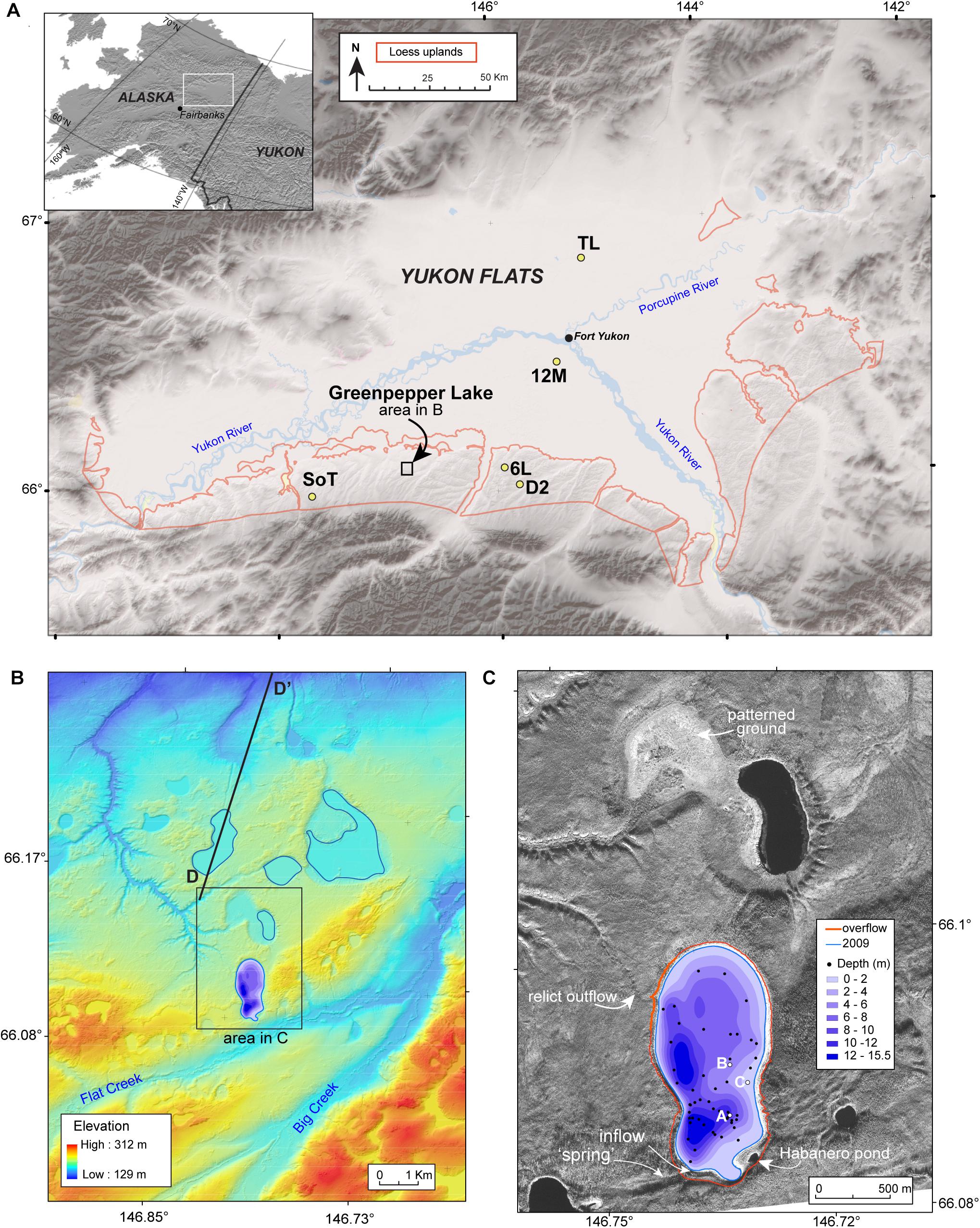
Figure 1. Map of the Yukon Flats, Alaska study area: (A). The southern loess uplands are enclosed by the red line: TL, Track Lake; 12M, Twelvemile Lake; SoT, Sands of Time Lake; 6L, Six Loon Lake; D2, Dune Two Lake. (B) Bathymetric contour map of Greenpepper Lake (purple shading) is shown on a 5-m IFSAR digital elevation model of the Flat and Big Creek areas. The electromagnetic survey line D-D’ from Minsley et al. (2012) indicates a deep talik underneath the lake to the north of Greenpepper; blue outlines of modern lake levels indicate the two partially filled basins. (C) Bathymetry (purple shading) on black imagery (Digital Globe WV02) in June of 2009, prior to the July 2009 fire, showing the locations of the sediment cores (A–C), lake shorelines in 2009 (blue) and at the surface overflow elevation (red), and the ‘spring’ and inflow water sampling sites. Patterned ground is evident within the partially filled lake basin and the drainage channel intersects the same gully system as the raised relict outflow channel from Greenpepper Lake.

Study Area

Located within the boreal forest near the Arctic Circle, the Yukon Flats is a broad, low lying basin where the westward flowing Porcupine River joins the northward flowing Yukon River as it bends to the west (Figure 1). Along the lower slopes of the Yukon-Tanana Upland that borders the southern margins of the Yukon Flats, nearly contiguous and extensive loess overlies late Tertiary or early Quaternary alluvium (Williams, 1962). Stratigraphic analyses of this loess indicate ages from the early to middle Pleistocene (Begét, 2001; McDowell and Edwards, 2001; Matheus et al., 2003 and references therein) and the late Pleistocene (Froese et al., 2005) with geochemical evidence for sources from expanded glaciation in the Brooks Range to the north and the Alaska Range to the south (Muhs et al., 2018).

Williams (1962) reported that the southern marginal loess is perennially frozen 1–2 m below the surface and contains ground-ice as small veins, stringers, polygonal wedges and large irregular, tabular and polygonal masses, which was supported by observations made by Edwards et al. (2016). Airborne electromagnetic surveys reported by Minsley et al. (2012) included an observation line that crossed the southern loess margin and indicated thick permafrost (D-D’ on Figure 1B). Deep unfrozen zones occur below deep lakes and in creek valleys that could provide groundwater conduits to the flats (Williams, 1970).

The climate of the Yukon Flats supports permanently frozen ground with a mean annual temperature of ∼-6°C (Jepsen et al., 2013). Large seasonal temperature differences range from winter minima near -55°C and summer maxima of 35°C. Mean annual precipitation is ∼250 mm with slightly more than half falling as rain during the summer and early fall. The modern vegetation of the flats is a dynamic mosaic of open meadow, spruce forest (Picea glauca and P. mariana) and successional birch-aspen forest (Betula neoalaskana and Populus tremuloides). Tall shrubs include Salix and Alnus. The southern loess uplands are dominated by spruce and successional hardwoods with tree-line at ∼900 m a.s.l. in the White Mountains to the south.

Greenpepper Lake indents an area of high ground on the north side of Flat Creek, a tributary of Big Creek, mapped as an escarpment within the southern loess uplands by Williams (1962) (Figure 1A). The elongate, bell pepper shaped lake is ∼2 km in length and 750 m wide. We observed pervasive permafrost throughout the area near Greenpepper Lake. During July 2010, ground and airborne observations indicated extensive near-surface permafrost thaw along the southern lake margins, which had burned in 2009 (Supplementary Figure 1). Thawed silt was readily mobilized in sheet and stream flow down hillslopes across extensively burned areas to the south. At a point of surface discharge along the lake’s southern margins, a silt delta formed below slopes that were actively undergoing fracture and slump (seen as corrugated thermokarst slump features in imagery; Figure 1C). Airborne observations identified patterned ground in the partially drained lake basin to the north that is also evident in high-resolution imagery (Figure 1C).

The surface of Greenpepper Lake currently (2018) lies several meters below the surrounding land surface. A small, round water-filled depression of unknown depth, informally named here as Habanero Pond, lies near the southern lake margin. Along the northern and southern lake margins, steep loess bluffs, 3–5 m high, are fully or partially stabilized by vegetation. Lower terrain lies near the lake margins to the east and west. A dry outlet channel at an elevation of ∼211.5 m a.s.l. was identified on the ground within dense forest; its base is currently ∼4.5 m above the lake surface. The channel is evident in aerial photography and high-resolution imagery (Figures 1B,C). It converges with two other channels that emanate from three partially drained lakes to the north, and together these form a deep gully that in many locations appears dry and, in a few places, contains standing water.

Raised shorelines and relict outlet channels indicate the neighboring lakes to the north of Greenpepper were once larger and deeper, with water lost at some time in the past (Figures 1B,C). Based on the depth and elevation of the drainage channels and on recent observations of other “catastrophic” lake drainage (i.e., extensive lake drainage over hours to days), they likely lowered to the levels of their outlets by one or more episodes of rapid lake drainage, but they did not drain completely. In a nearby drainage event that occurred in 2013, an outlet channel cut down several meters to massive permafrost and then stopped lowering because the permafrost possibly acted as a physical and thermal barrier to further erosion (Josh Rose, 2016, personal communication; Paul Carling, 2018, personal communication). The presence of massive ice at depth may be a key reason for the abundance of partially full lakes across the southern marginal upland.

The differing histories of Greenpepper and adjacent lakes and their heterogenous surface features leads us to speculate that a locally complex hydrologic system may be operating. Greenpepper currently appears to undergo changes in lake level (Supplementary Figure 1) and a full lake to the north has a deep talik as revealed by an electromagnetic survey line (D-D’ on Figure 1B; Minsley et al., 2012). If a similarly deep unfrozen zone lies beneath Greenpepper, its level may be responding to local changes in subsurface hydrology and groundwater routes, which are linked to surface-water dynamics. Thus, deep taliks may influence individual lake levels via both filling and drawing down and, on occasion, filling of lakes may drive overflow and drainage, possibly through a series of lakes, as it did in 2013.

Materials and Methods

Bathymetry was determined at Greenpepper Lake from 60 global positioning system (GPS)-located, sonar-measured water depths that are shown relative to the elevation of the 2009 shoreline in Figures 1B,C. The relict shoreline elevation was determined from a 2-m interferometric synthetic aperture radar (IFSAR) Digital Elevation Model (DEM). Lake volumes and surface areas were calculated at 1.0-m depth increments using a kriging interpolation method within ArcGIS 3D Analyst; hypsometric results are shown in Table 1.

TABLE 1

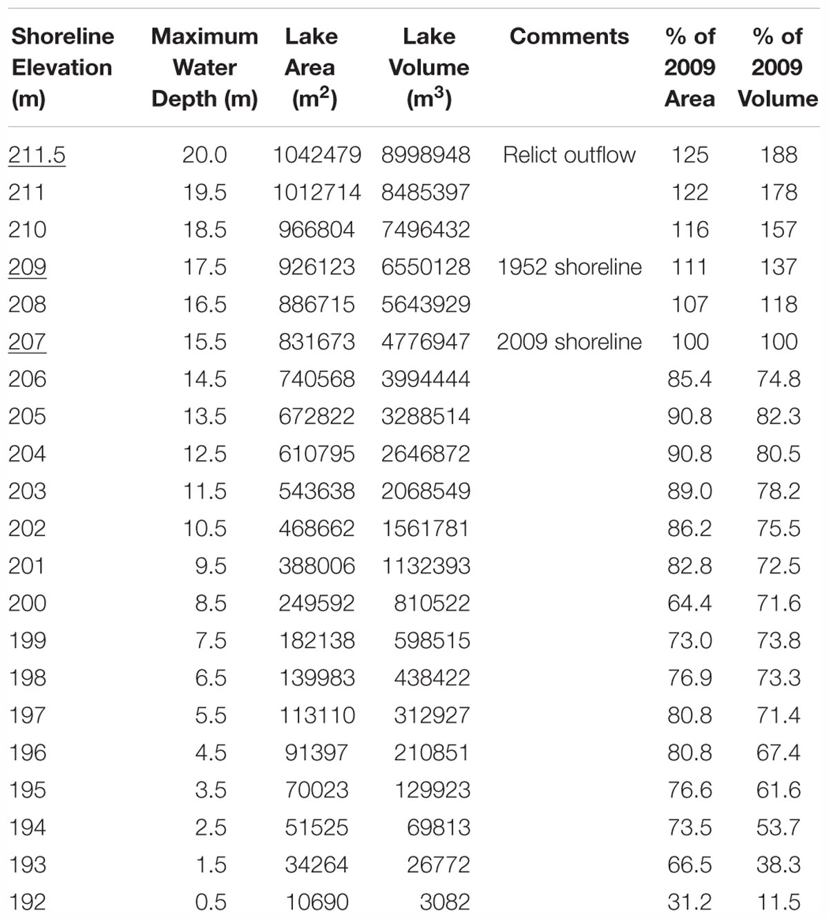
Table 1. Greenpepper Lake hypsometric estimates.

In July 2010, surface and water-column measurements of Greenpepper Lake temperature (T), pH, specific conductance (Spc) and dissolved oxygen (DO) were collected with a calibrated HydroLab Quanta^TM sonde, which has accuracies of ±0.15°C for T, ±0.2 units for pH, ±0.1% of Spc reading, and ±0.2 mg/L for DO. Greenpepper Lake water chemistry data for samples obtained in 2007 and 2008 are published in Halm and Guldager (2012). Near-surface water samples were collected in 2010 from the lake, Habanero Pond, the ‘spring’ and inflowing stream for isotope and major ion analyses in 30 ml high-density polyethylene (HDPE) Whatman^TM bottles and sealed with no headspace. Major ions for samples from Habanero Pond, ‘spring’ and inflowing stream (Table 2) were determined in 2018 on filtered and acidified (cations) aliquots from refrigerated archived samples at the U.S. Geological Survey Colorado Water Science Center, Denver, CO. Chloride, nitrate, and sulfate were determined using a Dionex ion chromatograph and calcium, magnesium, sodium, potassium, and silica were determined by a PerkinElmer inductively coupled plasma-atomic emission spectrometer (ICP-AES). All analytical runs have an uncertainty better than 5% based on analyses of blanks, replicates, and standard reference materials following U.S. Geological Survey quality assurance protocols (Fishman et al., 1994). Mineral saturation indices for lake water were calculated using PHREEQC (Parkhurst and Appelo, 1999); solute-based residence time estimates use the reactive mass-balance approach of Donovan (1994).

TABLE 2

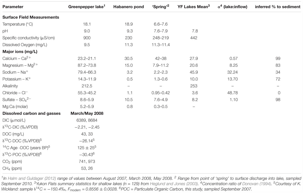
Table 2. Aqueous geochemistry of Greenpepper Lake.

Water samples for isotope analysis were filtered through 0.45-μm filters and analyzed using a Thermo Scientific, High Temperature Conversion Elemental Analyzer (TC-EA) interfaced to a Delta V Advantage mass spectrometer through the ConFlo IV system at Idaho State University Stable Isotope Laboratory, Pocatello, United States, ID. Four in-house standards, which are directly calibrated against Vienna Standard Mean Ocean Water 2 (VSMOW2), Standard Light Antarctic Precipitation 2 (SLAP2), and Greenland Ice Sheet Precipitation (GISP), were used to create a two-point calibration curve to correct the raw data and to monitor accuracy. Precision for δ²H and δ¹⁸O is better than ±2.0‰ and ±0.2‰ respectively. Random replicates represent ∼15% of analyzed samples and results fell within the range of analytical error. Water oxygen and hydrogen isotope results are reported in per mil (‰) as the relative difference of isotope ratios (δ) from the international measurement standard Vienna Standard Mean Ocean Water (VSMOW) defined by δ¹⁸O_H2O = [(¹⁸O/¹⁶O)_H2O/(¹⁸O/¹⁶O)_{V SMOW}] – 1 and δ²H_H2O = [(²H/¹H)_H2O / (²H/¹H)_{V SMOW})] – 1.

Sediment cores were obtained from a securely anchored floating platform in July 2010 from three locations, A, B, and C, with water depths of 10, 5, and 1.85 m respectively (Figure 1C). Core A was located slightly to the east of the deepest water depth of 15.5 m measured in the southernmost basin to avoid any potential slumped sediments from the steep slope along the southwest shoreline. Core B is located on the gently grading slope on the east side of the northern basin and Core C was within 10 m of the eastern shoreline in the littoral zone. Cores with an undisturbed sediment-water interface were obtained at all three locations using a customized polycarbonate tube fit with a piston and extruded in the field at 0.5-cm increments (Glew et al., 2001). Lower sediments were obtained using modified Livingstone and ‘Bolivia’ coring devices.

Following whole-core magnetic susceptibility measurements at 1-cm increments using a Bartington susceptibility meter, the cores were split, imaged with a digital line-scanner with cross-polarized filters, sampled for petrographic smear slides, and visually logged on the basis of Munsell color, sedimentary composition, structure, and biogenic features at LacCore, at the University of Minnesota, Minneapolis, MN, United States (Supplementary Figure 2). Sediment classification of lithostratigraphic units are based on color, composition and structure, and petrographic smear slide mineral identification according to Schnurrenberger et al. (2003). Dry bulk density was determined on contiguous 1-cm³ samples taken at 0.5- and 1.0-cm increments. Percent organic and inorganic carbon was determined from dry, pulverized subsamples using total carbon (TC) and total inorganic carbon (TIC) measurements by a UIC Inc.^TM carbon dioxide coulometer (Engleman et al., 1985) at the U.S. Geological Survey, Lakewood, CO, United States. Accuracy and precision and sample reproducibility for both TC and TIC is 0.1%. Percent organic carbon was calculated as the difference between TC and TIC and converted to percent organic matter by a factor of 2.5, an approximation based on the molar fraction of carbon to hydrocarbons that make up lipids, carbohydrates and proteins (Meyers and Teranes, 2001). Biogenic silica (bSiO₂) was determined from a single extraction of silica by 0.1 M Na₂CO₃ and modified molybdate-blue spectrophotometry (Mortlock and Froelich, 1989) at Idaho State University Department of Geosciences, Pocatello, ID, United States. The absorbance is normalized to sediment mass and sedimentary silicon content is converted to biogenic opal by a factor of 2.4, assuming 10% water in biogenic silica by weight. All results have an estimated error of <5%, calculated as a coefficient of variation, based on one blank, one sample replicate, and three standard analyses for every 25 samples.

Subsamples for organic carbon (OC) and organic nitrogen percentages used to calculate organic C/N ratios, and for OC isotope analyses were acidified with 1 N HCl, rinsed to neutral, freeze dried and pulverized for combustion to CO₂ and NO₂ by a Carlo Erba^TM CN elemental analyzer coupled with a Finnigan Delta^TM Advantage isotope ratio mass spectrometer at the Idaho State University Stable Isotope Laboratory, Pocatello, ID, United States. Analytical precision for both OC and nitrogen percentages, calculated from analysis of standards distributed throughout each run, is <0.5%. OC isotope ratios are reported in per mil (‰) as the relative isotope-ratio difference from the international standard Vienna Pee Dee Belemnite (VPDB), defined by δ¹³C_Org = [(¹³C/¹²C)_Org/(¹³C/¹²C)_{V PDB}] - 1. Analytical precision, calculated from standards distributed throughout each run, is ±0.2‰.

Pollen samples throughout core B were analyzed at ∼20-cm intervals through the upper 120 cm and at ∼10-cm intervals through the basal 60 cm at the University of Southampton, United Kingdom; four samples were scanned for pollen (low counts) from core A basal silts at 194, 197, 202, 204 cm depth. These samples were also analyzed for macrofossils (>150 μm size fractions) at the U.S. Geological Survey, Lakewood, CO, United States. Core B sample volumes were all 1-cm³ whereas 4-cm³ was sampled for the organic-poor basal silts of core A. Preparation, identification and counting followed the conventional methods of Faegri and Iverson (1989). Reference material held at the University of Southampton was consulted as required. The pollen sum was >300 terrestrial pollen grains, except in the lowermost two units of core B and for the scan counts at the base of core A, where concentrations were extremely low. The pollen percentage diagram for core B was plotted using TILIA software (Grimm, 1990). Core B macro-charcoal (>125 μm) was counted from 1-cm³ samples taken at 4-cm intervals at the University of Southampton, United Kingdom. Samples were deflocculated in 10% sodium pyrophosphate for 24 h. A 5% bleach solution cleared the color from organic matter other than charcoal. Samples were then sieved and counted at x20 magnification. All charcoal pieces in the sample were counted, thereby providing charcoal concentrations (count/cm³).

The sediment chronologies are based on accelerator mass spectrometry (AMS) radiocarbon measurements on fine charcoal and selected terrestrial and aquatic macrofossils graphitized at the Institute for Arctic, Antarctic and Alpine Research at the University of Colorado, Boulder, CO, United States (CURL lab numbers), the Lawrence Livermore National Laboratory, Livermore, CA, United States (CAMS lab numbers), and the U.S. Geological Survey Radiocarbon Laboratory, Lakewood, CO, United States (USGS lab number); pollen extracts, prepared at LacCore, were dated at a few stratigraphic intervals where no macrofossils were present (Brown et al., 1993). Both measured and calibrated radiocarbon ages (Calib 7.0.1; Stuiver and Reimer, 1993) are reported but only calibrated ages (cal yr BP; 1950) are used for discussion (Table 3). ²¹⁰Pb was measured on 0.5 cm intervals for core A from the surface to 26 cm depth at the St. Croix Research Station of the Science Museum of Minnesota (Table 3). Although maximum values of 10 pCi/g are considered low, they are typical of high-latitude values and similar to those measured from recent sediments at nearby Track and Twelvemile Lakes (Figure 1; Anderson et al., 2018). There is a well-defined break between sediment containing unsupported ²¹⁰Pb below the relatively smooth down-core declines in supported ²¹⁰Pb. ²¹⁰Pb-ages were determined by a Constant Rate of Supply (CRS) age model (Appleby, 2001). An age model for core A was generated with ²¹⁰Pb and radiocarbon measurements of terrestrial macrofossils using the Bayesian software Bacon (v2.3; Blaauw and Christen, 2011, 2013; Supplementary Figure 3) which uses the most recent calibration curve (Reimer et al., 2013) and default prior assumptions.

TABLE 3

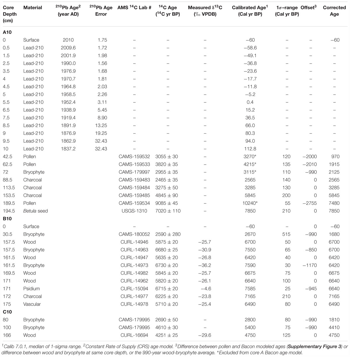
Table 3. Greenpepper lake chronostratigraphic data.

Results

Bathymetry and Limnology

Water column measurements indicate that Greenpepper Lake is dimictic with summer thermal stratification indicated by declines in temperature, DO, Spc and pH between 4 and 6 m water depth (Figure 2A). The hypolimnion below the thermocline is anoxic with a temperature of 6°C, pH of 8.75, and Spc values near 1000 μS/L. The surface pH value of 9 is higher than most Yukon Flats (YF) lakes and surface Spc values of 900 μS/L are two times higher than average (Table 2). Calcium and alkalinity concentrations are slightly lower than average whereas sodium, magnesium and chloride are elevated. The lake is supersaturated in carbon dioxide and methane and has high concentrations of dissolved organic (DOC) and inorganic carbon (DIC); a DOC age of ∼125 years was determined by the National Ocean Sciences Accelerator Mass Spectrometer at the Woods Hole Oceanographic Institution (Wickland, 2018 personal communication).

FIGURE 2

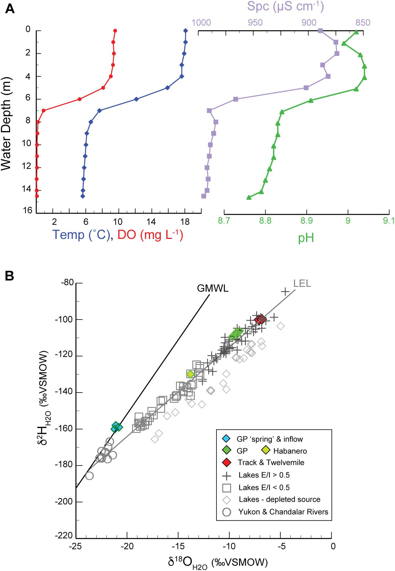
Figure 2. (A) Greenpepper Lake water column physical properties measured within the core A basin in July 2010; temperature [Temp (°C)], dissolved oxygen [DO (mg L^-1)], specific conductivity [Spc (μS cm^-1)], and pH. (B) Oxygen and hydrogen isotope values for Greenpepper Lake (dark green diamonds), Habanero Pond (light green diamond), the ‘spring’ and inflow (blue diamonds), Track and Twelvemile Lakes (red diamonds), with reference Yukon Flats lake and river samples from Anderson et al. (2013; open symbols) and the Global Meteoric Water Line (GMWL). Reference lakes are characterized by evaporation to inflow ratios (E/I) as either open (E/I < 0.5 = open squares) or closed (E/I > 0.5 = crosses). Regression for open and closed lakes form a Local Evaporation Line (LEL) with a slope of 4.88. Reference lakes with more isotopically depleted sources such as snow and/or permafrost thaw form a third group (open diamonds) and are not included in the LEL regression.

The bathymetric study identified two steep-sided basins ∼15.5 m deep immediately below the lake’s western margins separated by a narrow sill between 5 and 6 m water depth (Figure 1C). Most other areas have water depths of ∼5 m and low-gradient slopes dip toward the depocenters to the west. Littoral shorelines are lined with horsetail (Equisetum sp.) and sedge (Scirpus sp.) and water depths between 3 and 1 m host abundant pond weeds (Potamogetonaceae). Cloud-free historic air photos and remotely sensed imagery (air photography, LandSat, SPOT, and Digital Globe) for ice-free months are available for Greenpepper for the years 1952, 1977, 1978, 1990, 2008, 2009, 2012, and 2017 (Supplementary Figure 1). They indicate higher lake levels during the early 1950s, while since ∼1990 the shoreline has been near the 2009 elevation.

Surface inflow to the lake in the form of a permanent stream has not been observed between 2007 and 2018, either in the field or from historic imagery, with the exception of the small point of surface discharge observed in 2010; this represented converging silt-rich sheet-flow originating from a thawed slump-block area within the burn along the southern lake margins (Figure 3A). The source of the surface stream was an active point of subsurface discharge within the banks of a thaw-collapse channel, found ∼100 m upslope to the southwest from this location and is referred to here as a ‘spring’ (Figure 1C). It is unknown if this area has been a perennial source of inflow into the lake prior to the 2009 fire or if it has continued to supply water since.

FIGURE 3

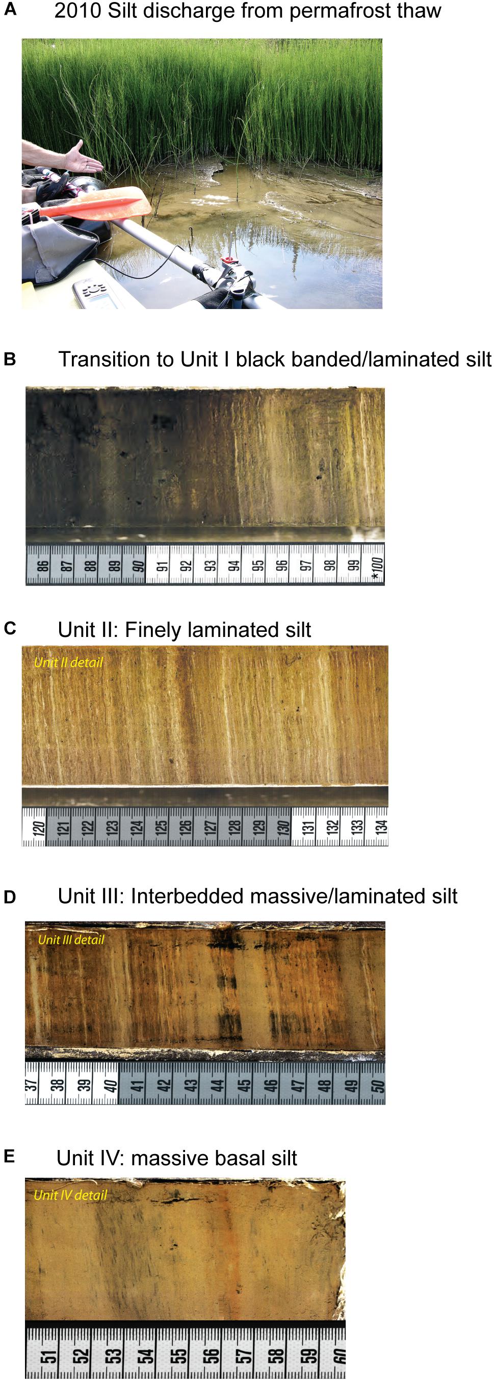
Figure 3. (A) Point of surface discharge into Greenpepper Lake observed in 2010 with high silt loads originating from southern lake margins undergoing active permafrost thaw following a July 2009 forest fire (Figure 1C and Supplementary Figure 1). High-resolution image details from the four major lithologic facies identified in core A with scale units in cm. (B) Uppermost Unit I black banded/faintly laminated silt and the transition to upper Unit II; (C) Unit II finely laminated brown silt; (D) Transition Unit III with interbedded massive silt with finely laminated silt intervals; (E) Massive, brown basal silt Unit IV. Image brightness and contrast was adjusted to enhance sediment features.

The lake has no surface outflow and lake-water isotope compositions are highly enriched in heavy isotopes relative to lakes in the region, indicating significant water loss by evaporation (Figure 2B). The Yukon Flats local evaporation line (LEL) has a slope of 4.89 (R²= 0.88) for lakes sourced by precipitation (from Anderson et al., 2013) and the intercept with the Global Meteoric Water Line (GMWL) has a δ¹⁸O value of -23‰. Greenpepper ‘spring’ and inflow water isotope values are positioned slightly higher on the GMWL, with a δ¹⁸O value of -21‰, and their linear regression with lake water has a slightly lower slope than the LEL (4.37, R² = 0.99). The extent of water loss by evaporation at Greenpepper Lake is further illustrated by applying the isotope mass balance methods discussed in Gibson et al. (2016) used to estimate the ratio of lake evaporation to inflow (E/I). The Greenpepper E/I value of 0.96 (from Anderson et al., 2013) indicates that water loss by evaporation during the ice-free season is nearly two times the amount of inflow gain.

Comparison of major-ion concentrations of Greenpepper Lake and inflow (Table 2) when converted to molar compositions indicate a notable shift in molar Mg:Ca from near 0.5 (inflow) to between 5 and 6 (lake). This is among the highest known regionally and largely reflects precipitation of calcium carbonate within the lake water column, promoted by evaporative concentration and dissolved carbon equilibration, and its burial in sediments. There is also a nearly four-fold increase in specific conductance, a proxy for total dissolved solids (TDS). Chloride ion, considered approximately conservative in its behavior in dilute lakes, is elevated 50 to 100-fold relative to inflow, reflecting the balance of conservative solutes. If chloride is delivered solely by inflow and previous net evaporation estimates are correct (23 cm in Anderson et al., 2018), then lake hydraulic residence times are ∼25 years. Shorter residence times only arise if there are large, unrecognized chloride influxes from atmospheric or geologic sources. This result is consistent with the residence times implied by the isotopic enrichment and the relatively old radiocarbon age of DIC; old DIC may be accounted for through the combined effect of long hydraulic lake residence times and contribution of dissolved carbon from respiration of ancient remnant organic matter in the watershed and from thawed permafrost sources.

Lake Sediments

Sediment cores were obtained on a transect from deep to shallow water at depths of 10, 5, and 1.85 m below modern levels (BML). At each core location, overlapping stratigraphic intervals were visually matched and confirmed or adjusted by bulk sedimentary data to form composite core sections (Supplementary Figure 2). Core A is 205 cm in length (Figures 4, 5), core B is 188 cm (Figures 5–7) and core C is 195 cm (Figures 5, 8). Below are detailed lithologic unit descriptions, including smear slide mineralogy, and their timing and environmental interpretation which are briefly summarized in Table 4.

FIGURE 4

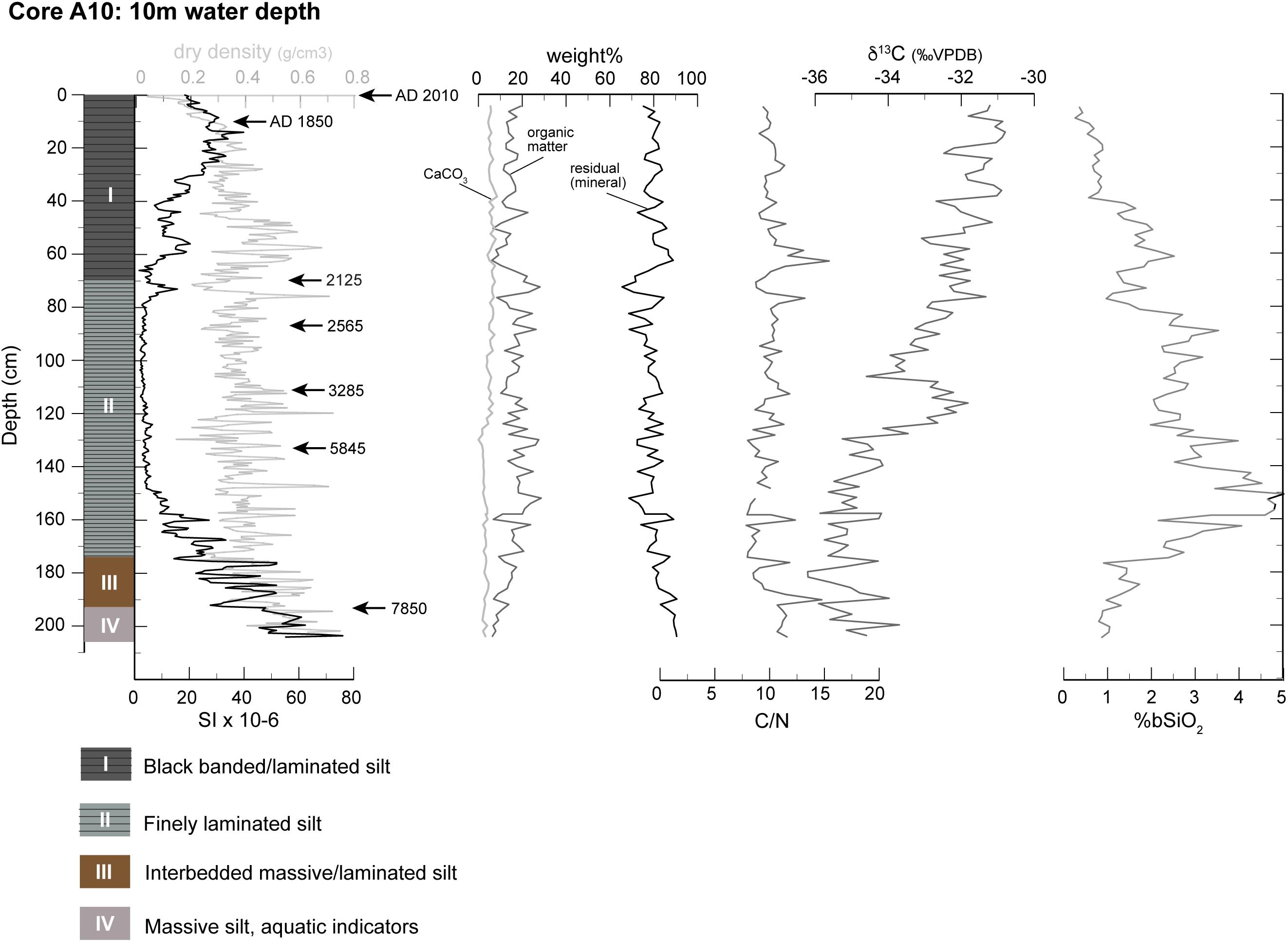
Figure 4. Sediment core A lithology, physical and geochemical properties, and radiocarbon ages in cal yr BP (arrows): magnetic susceptibility (SI × 10^-6), dry bulk density (g/cm³), weight percentages (weight%) calcium carbonate (CaCO₃), organic matter, and residual mineral matter, organic C/N ratio, organic matter δ¹³C values (‰VPDB), and weight percentages of biogenic silica (%bSiO₂).

FIGURE 5

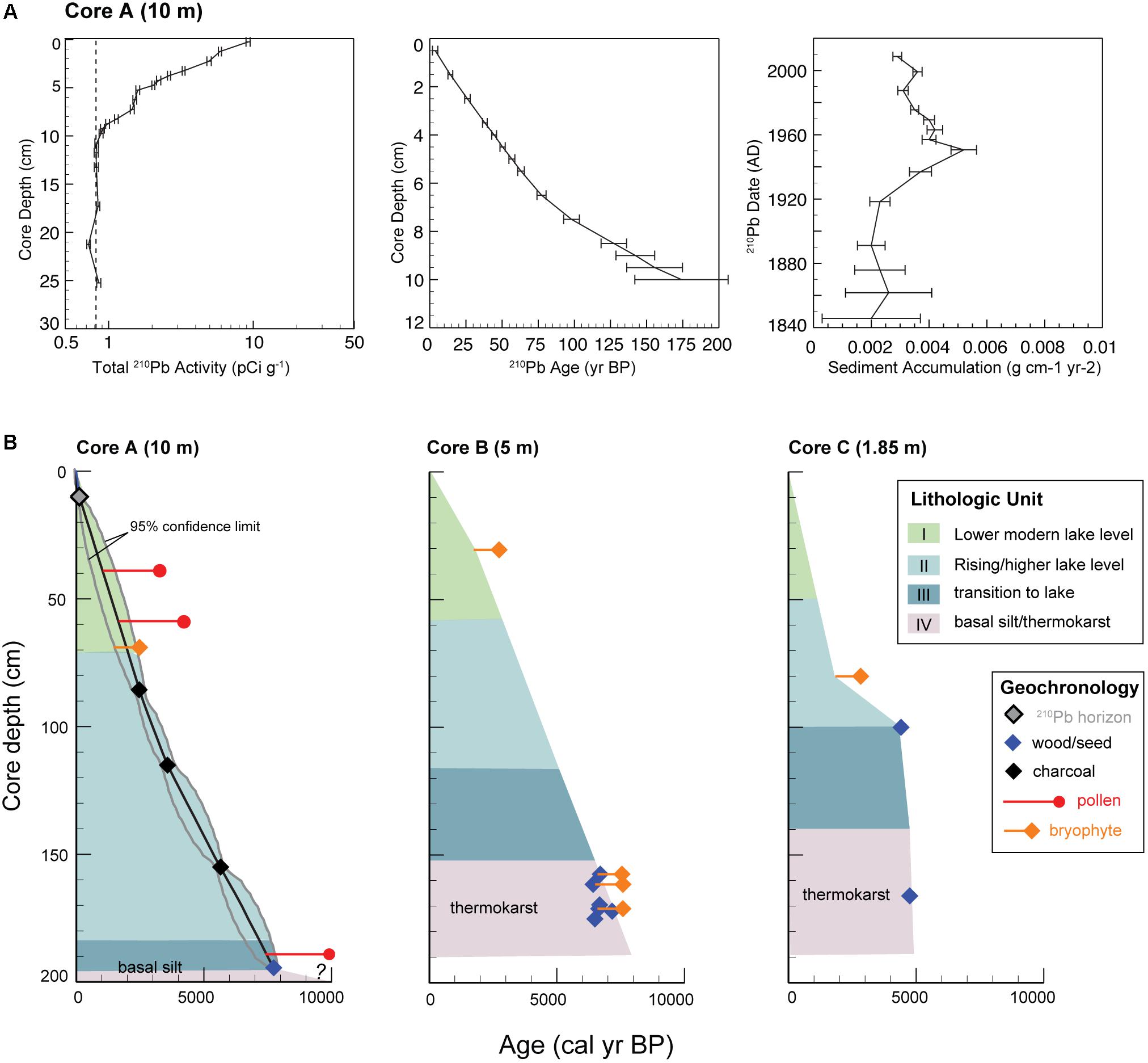
Figure 5. (A) Sediment core A ²¹⁰Pb activity, CRS ages, and sediment accumulation rates with error ranges. (B) Core A (10-m water depth) Bacon age model (mean is black line and gray lines indicated 95% confidence limits; Supplementary Figure 3) shown with lithologic units and all calibrated radiocarbon ages (cal yr BP) for core B (5-m water depth) and core C (1.85 m water depth); charcoal (black), pollen (red) and aquatic bryophytes (orange). The radiocarbon age symbols are larger than calibrated 1-sigma age errors and tails on the pollen and bryophyte symbols reflect age offsets (Table 3).

FIGURE 6

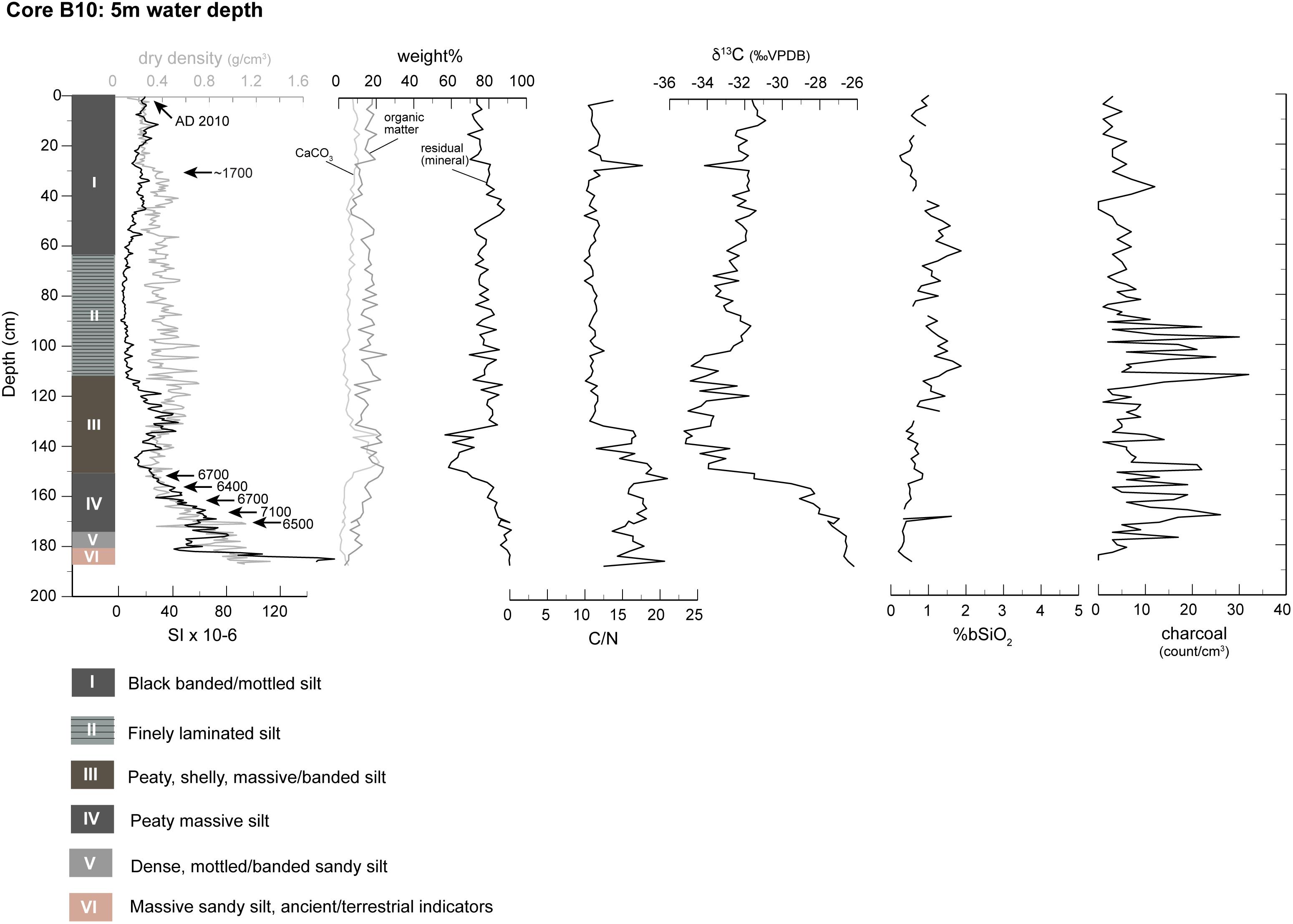
Figure 6. Sediment core B lithology, physical and geochemical properties, and radiocarbon ages in cal yr BP (arrows): magnetic susceptibility (SI × 10^-6), dry bulk density (g/cm³), weight percentages (weight%) calcium carbonate (CaCO₃), organic matter, and residual mineral matter, organic C/N ratio, organic matter δ¹³C values (‰ VPDB), weight percentages of biogenic silica (%bSiO₂), and charcoal abundance (count/cm³).

FIGURE 7

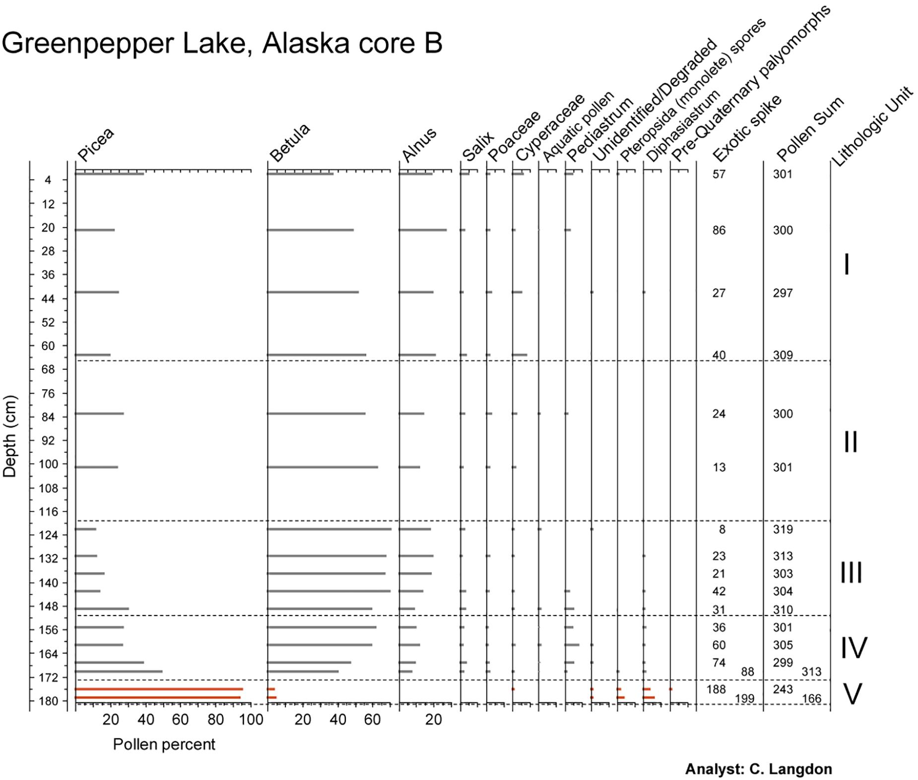
Figure 7. Core B pollen type percentages by core depth with pollen sum amounts. Basal unit V values are highlighted in orange.

FIGURE 8

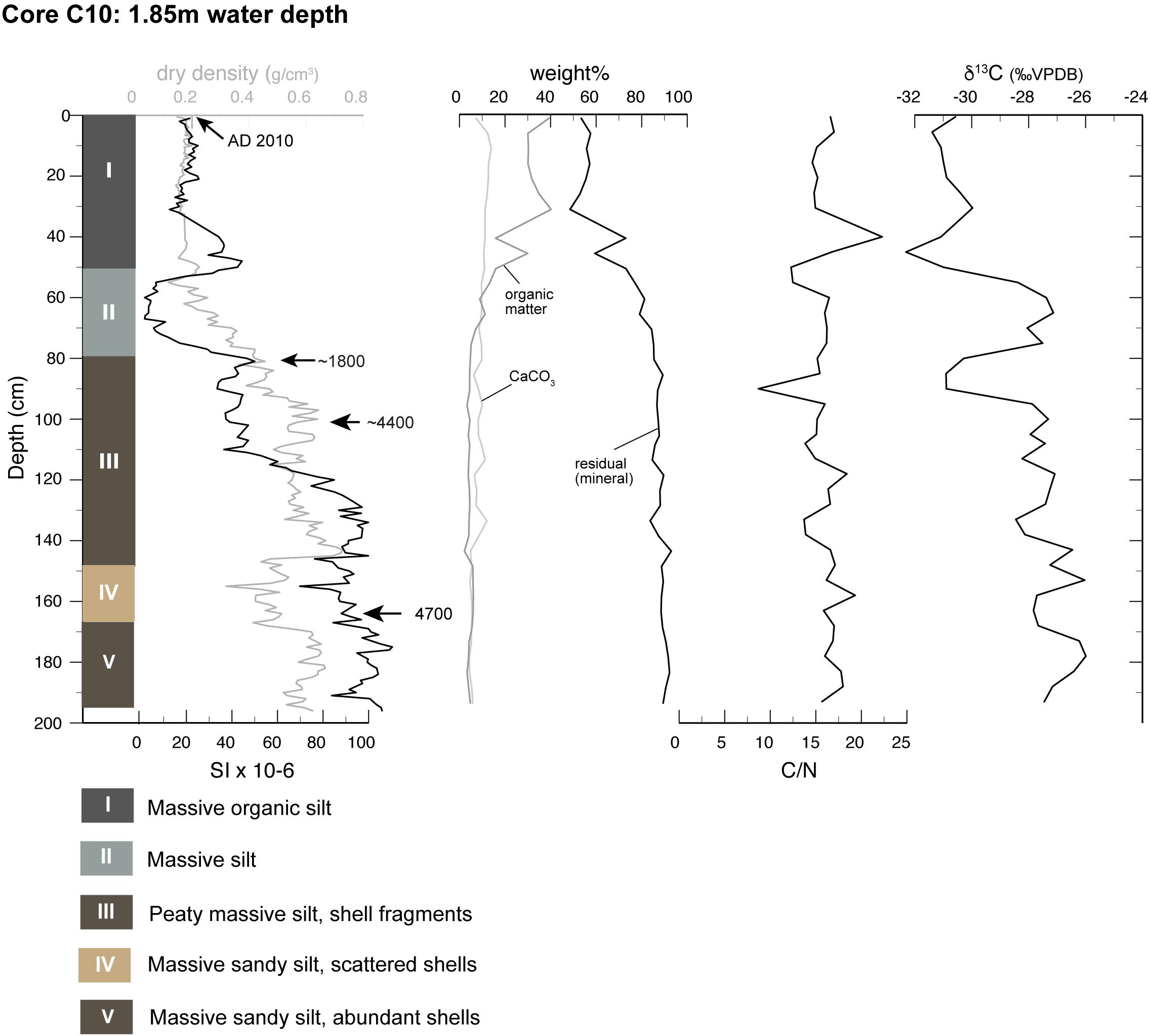
Figure 8. Sediment core C lithology, physical and geochemical properties, and corrected radiocarbon ages in cal yr BP (arrows): magnetic susceptibility (SI × 10^-6), dry bulk density (g/cm³), weight percentages (weight%) calcium carbonate (CaCO₃), organic matter, and residual mineral matter, organic C/N ratio, organic matter δ¹³C values (‰ VPDB).

TABLE 4

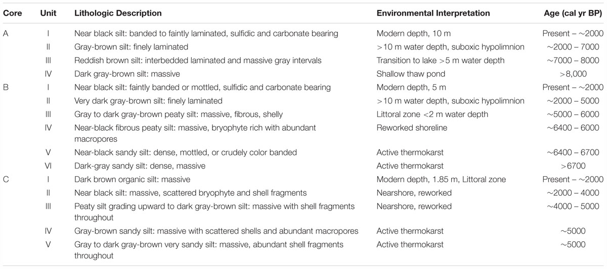
Table 4. Greenpepper Lake sediment core lithology, interpretation, and estimated ages.

Core A (10 m BML)

Basal unit IV (205-195 cm depth; Figures 3E, 4; >8,500 cal yr BP based on pollen stratigraphy – see below) is composed of near-massive, clayey and slightly calcareous dark gray-brown medium silt. Bulk sediments are high in magnetic susceptibility (40–60 SI), and dry bulk density (∼0.6 g/cm³), and low in bSiO₂ (1%) and calcium carbonate (<5%). Organic matter is present in trace quantities as very fine fragmentary material; C/N ratios are ∼11 and δ¹³C values vary between -33 and -34‰. In smear slides, mafic minerals are relatively abundant (est. 15–20% in silt size range) and erosionally resistant accessory minerals (zircon, rutile) are observed in addition to diagenetic sulfide minerals, including both highly reactive monosulfides and abundant pyrite framboids up to 20 μm in diameter. Other diagenetic indicators, such as opaque coatings on quartz and feldspar grains, are common. The silt grains are dominantly sub-angular with modal size near 30 μm. The presence of microzooplanktonic Daphnia ephippia (water flea egg cases) indicates standing water (permanent or seasonal). Pollen at 204 cm is dominated by Betula; Alnus is absent and there are abundant fungal hyphae. Fluctuating Picea percentages from 204 cm (<10%) to 202 cm (29%) and 197 cm (<10%) may partly reflect reworked sediments as many grains in all samples are poorly preserved (Supplementary Table 1). Alternatively, the fluctuations could reflect a pond edge environment, where large amounts of floating Picea grains are blown shoreward. Despite these uncertainties, the high Betula count and lack of Alnus indicates the sediments are older than ∼8,500 cal yr BP, according to ages that bracket similar assemblages at 6L and Sands of Time (SoT) lakes (Edwards et al., 2016).

Unit III (195-173 cm depth; Figures 3D, 4; ∼8,000 to 7,000 cal yr BP) is a transitional sequence, characterized by alternating cm-scale bands of finely laminated reddish-brown silt and massive gray brown silt. High magnetic susceptibility and dry bulk density and low bSiO₂ and calcium carbonate are similar to Unit IV. Organic matter was present in trace quantities as very fine fragmentary material; C/N ratios fluctuate near ∼10 and δ¹³C values vary between -34 and -36‰. The prominent gray bands, composed of well-sorted medium silt, lack much of the obvious reactive Fe apparent in other components. Elsewhere, evidence is widespread for diagenesis involving Fe phases (oxide coatings on sand grains, co-occurring ferric oxides and sulfides; vivianite occurrences) and carbonates (resorption textures). The earliest (lowermost) laminated sequence at 194 cm has abundant Daphnia sp. in addition to rare insect parts and a birch seed (Betula. sp.) that provided an age of 7850 cal yr BP. The pollen is dominated by Betula (74%) and Picea (22%), and one grain of the aquatic macrophyte Myriophyllum was counted.

Unit II (173-70 cm depth; Figures 3C, 4; ∼7,000 to 2000 cal yr BP) is a deep lacustrine facies of continuous finely laminated (<1 mm) very dark gray-brown, moderately calcareous and medium grained silt. The laminae are distinct but frequently irregular and often appear knotted or crumpled as well as bundled into 1–5 cm bands by oxidized Fe phases. The contact with lower Unit III is reflected by lower magnetic susceptibility (<10 SI) and dry bulk density (∼0.35 g/cm³), and higher bSiO₂ (5%), organic matter (10–20%) and calcium carbonate (∼5%). Notwithstanding the higher bSiO₂ percentages, diatoms rarely occur in smear slides. Organic matter is amorphous and the only identifiable fragmentary material is bryophytic; organic C/N ratios of ∼10 are stable throughout the unit as δ¹³C values increase up core to >-33‰. Purified pollen provided an age of 10,240 cal yr BP at 189 cm, but comparison with the Betula seed age indicates that the pollen age is at least ∼2700 years too old (Table 3 and Figure 5). The age model indicates that the top of the unit dates to ∼2080 cal yr BP, which is supported by a corrected bryophyte age of 2125 cal yr BP. Occasional laminae and nodules are dominated by fine (<10 μm) endogenic carbonate, typically twinned. Occasional gray laminae are dominated by angular to sub-angular siliciclastic medium silt with minor carbonate. Peaks in magnetic susceptibility correspond to concentrations in reactive Fe textures with abundant opaque framboids (sulfides) and Fe oxides as crystallites and grain coatings. The initial near-black core face color oxidized within 72 h as further indication of readily oxidized Fe-monosulfide minerals.

Unit I (70-0 cm depth; Figure 3B; ∼2000 to -60 cal yr BP) is a lacustrine lithology that reflects a shift to near-black silt with diffuse to discontinuous lamination. There is an increase in magnetic susceptibility (∼40 SI) and decline in bSiO₂ as percentages of carbonate and OC remain unchanged. Occasional pulses of medium to coarse-grained sub-angular silt occurring as 1-mm gray clastic laminae with mafic minerals and detrital zircons correspond to a rise in magnetic susceptibility at 75-70 cm (20 SI) as the laminations become less distinct, and at 60-58 cm, where they are prominent. Carbonates include diverse endogenic forms, apparent detrital grains and occasional diagenetic nodules. Recognizable diatoms are absent and organic matter is amorphous. Organic C/N ratios decline slightly (∼9.5 to 9) as δ¹³C values increase to -31‰. The near surface Unit I sediments (<20 cm depth) are dark black watery silt that produced a distinctly pungent odor, although free of H₂S. The sediments contained dispersed mineral grains of pyrite, visible in bright sunlight and subsequently confirmed by x-ray diffraction (xrd) and petrographic observations of smear slides. The presence of highly reactive Fe-monosulfides prominently influence sediment color and its stability.

The ²¹⁰Pb age model confirmed the presence of an intact sediment-water interface (Figure 5) and indicates that the upper 10 cm of sediment accumulation occurred during the past ∼175 years (0.06 cm/yr), including a doubling of mass accumulation (g cm^-1 yr^-2) between AD 1920 and 1950. The average core A sedimentation rates based on the depths of the ²¹⁰Pb horizon and the charcoal ages used in the Bacon model is ∼0.03 cm/yr. Purified pollen from Unit I at 42.5 and 62.5 cm depth produced stratigraphically ordered ages of 3270 and 4215 cal yr BP, respectively, with reasonably consistent sedimentation rates of ∼0.02 cm/yr (Figure 5). However, comparison with modeled ages of 1050 and 1710 cal yr BP (Supplementary Figure 3) indicates that they are likely ∼2000 and 2110 years too old, respectively. Although it is not certain, the old pollen extract ages obtained in this study likely reflect the inclusion of ancient remnant organic matter fragments from the watershed and thawed permafrost sources.

Core B (5 m BML)

Basal Unit VI (187 to 180 cm depth; Figures 5–7; 6700 to 6400 cal yr BP) is massive dark-gray slightly sandy silt, and the overlying Unit V (180 to 175 cm depth) consists of slightly sandy, crudely banded silt (50–60 μm modal grain size range). Both units are compact and micaceous, with angular to sub-angular coarse silt, and minor carbonate and fragmentary organic matter. Abundant biotite (chlorite?) grains have opaque and hematitic coatings. Other mafic minerals are common and trace amounts of weathering resistant heavy minerals, such as rutile, occur. Magnetic susceptibility and dry bulk density values are high (140 to 60 SI, and 1.1 to 0.8 g/cm³) and percentages of bSiO₂, organic matter and carbonate are low (<1%, <5%, <10%, respectively). Charcoal concentrations are low (<5 count/cm³), and low pollen/spore counts (150–250 grains) are dominated by Picea, plus monolete spores, Diphasiastrum spores, and pre-Quaternary palynomorphs (Figure 7). Wood pieces, aquatic bryophytes, and Pisidium shells from the same depths (157.5, 161.5, 169, and 171 cm) had ages between 7600 and 6700 cal yr BP (Table 3). The wood ages of 6700, 6420, 6675, and 6640 cal yr BP with increasing depth are consistently younger than the paired aquatic macrofossils by ∼850 to 1170 years (average 990 years) and most accurately date the timing of this ‘trash’ layer formation to ∼6400–6700 cal yr BP.

Unit IV (175 to 150 cm depth; Figures 5–7; ∼6400 to ∼6000 cal yr BP) transition is marked by a distinct contact with near-black, massive, moderately calcareous, very silty fibrous peat with abundant macrofossils of bryophyte, wood, charcoal, and Pisidium shells. Bryophyte fragments increase in abundance and preservation upward. Magnetic susceptibility and dry bulk density abruptly decline (<20 SI, 0.35 g/cm³) as percentages of organic matter and carbonate begin to increase, with high C/N ratios (15–20) and declines in δ¹³C values from -27 to -34‰. Diverse carbonate forms include fine (<10 μm) twinned endogenic laths and blocky detrital grains. Charcoal counts rise (10–20 count/cm³), as do pollen percentages with an assemblage dominated by Beluta, Picea, and rising Alnus. The first aquatic indicators (Pediastrum cell nets) in the core B pollen record appear in unit IV.

Unit III (150 to 112 cm depth; Figures 5–7; ∼6000 to ∼5000 cal yr BP) is a transition lithology with a distinct contact to dark gray-brown crudely banded calcareous silt with abundant gastropod shells. Transition into this unit is reflected by a rise in magnetic susceptibility (30–40 SI), dry bulk density (0.4 g/cm³), and organic matter and carbonate percentages (20%) with high C/N ratios (15–20) and low δ¹³C values (-35‰). Carbonate occurs in diverse forms including fine, irregular silt, complex micritic aggregates, and subordinate but prominent large (>30 μm) ellipsoidal scales. Charcoal counts decline (5–10 count/cm³) and the pollen assemblage is dominated by Beluta (60%), with Picea and Alnus both 10–15%. Pediastrum values decline.

Unit II (112 to 65 cm depth; Figures 5–7; ∼5000 to ∼2000 cal yr BP) is a lacustrine lithology with a gradational contact characterized by upward development of finely laminated and banded dark gray-brown, moderately calcareous, silt. Prominent gray laminae are well-sorted angular to sub angular silt with prominent mafic minerals, and trace occurrences of zircon and rutile. Very thin, clotted laminae dominated by twinned endogenic carbonate occur episodically throughout. Magnetic susceptibility declines (<10 SI) and dry bulk density values stabilize (0.3 and 0.5 g/cm³) as bSiO₂ percentages rise slightly (1–2%), and percentages of carbonate decline (<10%) and percentages of organic matter, evident as fine fragmentary material and occasional coarser plant material, stabilize (10–20%). C/N ratios stabilize at a lower value of 10 and δ¹³C values rise slightly before stabilizing near -32‰. Charcoal concentrations in the lower half of the unit are significantly higher (up to 30 count/cm³) and then decline to low values (<15 count/cm³). Pollen is dominated by Betula, Picea, and Alnus.

Unit I (65 to 0 cm depth; Figures 5–7; ∼2000 to -60 cal yr BP) is a lacustrine lithology of near-black medium silt where gradational loss of laminae to a mottled texture is accompanied by a rise in magnetic susceptibility (30–40 SI), declining dry bulk density (0.3 g/cm³), and a slight rise in organic matter percentages (15–20%). Mineralogy is sulfidic and moderately calcareous while the silt is dominated by angular to sub-angular quartz and feldspar with subordinate pyroxene and other mafic minerals. Opaque phases include framboidal pyrite (20 μm in diameter) and reactive Fe-monosulfides. Charcoal counts remain generally low, and the pollen continues to be dominated by Betula, Picea and Alnus. Cyperaceae pollen is present at 5–10% and Pediastrum increases in the uppermost levels.

Core C (1.85 m BML)

Core C was taken within the littoral zone in an area of abundant submerged vegetation, and the five recognized lithostratigraphic units all belong to near-shore or littoral facies.

Basal units V (195 to 168 cm depth) and IV (168 to 143 cm depth; Figures 5–8; ∼5000 cal yr BP) are gray-brown massive to crudely banded, locally mottled, slightly calcareous, sandy silt with abundant shell fragments. Both units are characterized by high magnetic susceptibility (80–100 SI) and high dry bulk density (0.4–0.6 g/cm³). Percentages of OC and carbonate are low (<10%), C/N ratios are high (15–20) and δ¹³C values are high (-28 to -26‰). A radiocarbon age from wood at 166 cm depth of 4750 cal yr BP dates the reworked deposition (Table 3).

Unit III (143 to 80 cm depth; Figures 5–8; ∼5000 cal yr BP) is reflected by a distinct contact to moderately calcareous peaty silt which grades upward to dominantly silt, as reflected by step declines in magnetic susceptibility, and dry bulk density, but little change in percentages of carbonate and organic matter. A date of 5400 cal yr BP from a bryophyte overlaps with the age of wood at 166 cm depth in Unit IV, indicating significant reworking (Table 3). Diverse carbonate forms include fine irregular scraps, large tabular or ellipsoidal grains, and ostracode shell fragments. A prominent negative excursion in δ¹³C from values of -27 to -30‰ occurs near the top of the unit.

Unit II (80 to 50 cm depth; Figures 5–8; ∼4000 to 2000 cal yr BP) is marked by a gradational change to near black silt with scattered bryophyte and shell fragments which are reflected by an abrupt rise in δ¹³C values, declines in magnetic susceptibility and dry bulk density, and are dated by a bryophyte radiocarbon age of 2800 cal yr BP at 80 cm (Table 3).

Unit I (50 to 0 cm depth; Figures 5–8; ∼2000 to -64 cal yr BP) is marked by a subsequent rise in magnetic susceptibility (from 10 to 40 SI) between 55 and 45 cm depth that is followed by an increase in the percentages of organic matter and an abrupt decline in δ¹³C values (from -28 to -32‰). Near-surface sediments (<20 cm depth) are watery dark brown organic silts with abundant egg cases, shells, and living macrophyte fragments and roots.

Discussion

Evolution of Greenpepper Lake

Whereas the loess uplands represent a permafrost-affected landscape, not all lakes owe their origin primarily to thermokarst. For example, at Sands of Time Lake (SoT; Figure 1) silt accumulated during deglaciation between ∼22 and 13 ka in a small pond lying in a swale. However, many owe their origin, at least in part, to thaw of ground ice. Lakes that occupy basins within deep valleys rich in ground ice have proven to be deep where measured (>20 m), suggesting that for these lakes, valley ground ice is likely to have influenced their formation. In other lakes, such as Six Loon (6L) and Dune Two (D2), basal sediments strongly indicate thermokarst origins. Their central water depths are >10 m (similar to Greenpepper) and their basal silt is overlain by, and/or chaotically interbedded with, terrestrial organic shallow-water sediments or peat, which contains detrital plant material, aquatic molluscs, and charcoal. Chaotic sediment textures and structure are consistent with cryoturbation during the growth of shallow initial ponds that erode and promote collapse of older, underlying sediments. It should also be noted that while trash layers can be prominent, in other cases the boundary between underlying thawed silt (talik) and overlying lake sediments can be subtle. Furthermore, the dilution of aquatic indicators can occur due to the high mobility of thawed silt, its potentially rapid deposition, and/or winnowing by bottom currents or wind disturbance (Hopkins and Kidd, 1988), thus making the onset of lacustrine deposition difficult to determine via biotic proxies.

Our Greenpepper sediment record begins with a basal silt (core A Unit IV), which does not resemble a classic ‘trash’ layer. However, although silt represents the primary sediment component (∼80%) at all of the core sites throughout the lake’s history, the core A basal silts are unique because the gray color and massive texture are in contrast to the dark brown finely laminated facies above this unit (Figure 3). Trace macrofossils indicate that basal silt deposition occurred within an aquatic environment that was probably a shallow thaw pond, or even a seasonal pool. Thus, it is likely that additional basal sediments with a ‘trash’ layer were not retrieved due to equipment limitations. A thaw-pond or seasonal pool environment is consistent with relatively low C/N (10) and low δ¹³C values (-33 to -34‰) that reflect organic matter originating as aquatic phytoplankton (Figure 9). Low δ¹³C values could also reflect depleted carbon sources derived from methane-producing bacteria during early thaw phases (Wooller et al., 2012; Walter Anthony et al., 2014; Davies et al., 2016). The Betula seed age of 7850 cal yr BP provides an age for the transition from proto-Greenpepper thaw ponds to a deepening lake and the underlying pollen stratigraphy (dominated by Betula, some Picea, but virtually no Alnus) is similar to that of 6L and SoT lakes for the time period ca 9500 to 8500 cal yr BP. The modern bathymetry suggests two isolated thermokarst basins developed into deeper ponds with sufficiently suboxic hypolimnia for fine laminae preservation at the sediment water interface. Following this reasoning, the 10-m bathymetric contour is used in Figure 10A to draw a schematic of the early thaw pond shorelines by ∼9,000 cal yr BP that followed thermokarst initiation.

FIGURE 9

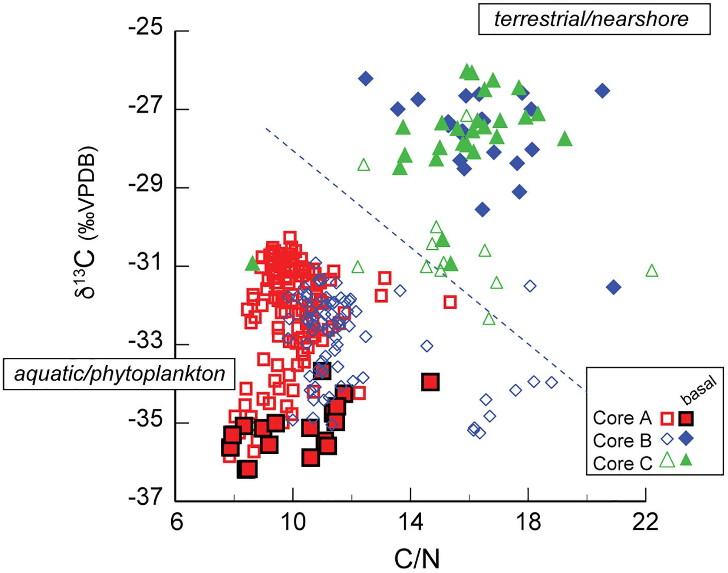
Figure 9. Sediment core organic matter C/N ratios and δ¹³C values with a delineation between aquatic/phytoplankton and terrestrial/nearshore organic carbon sources. Symbols for core A are red squares, core B are blue diamonds, and core C are green triangles, with solid symbols for basal sediments and open symbols for lacustrine muds.

FIGURE 10

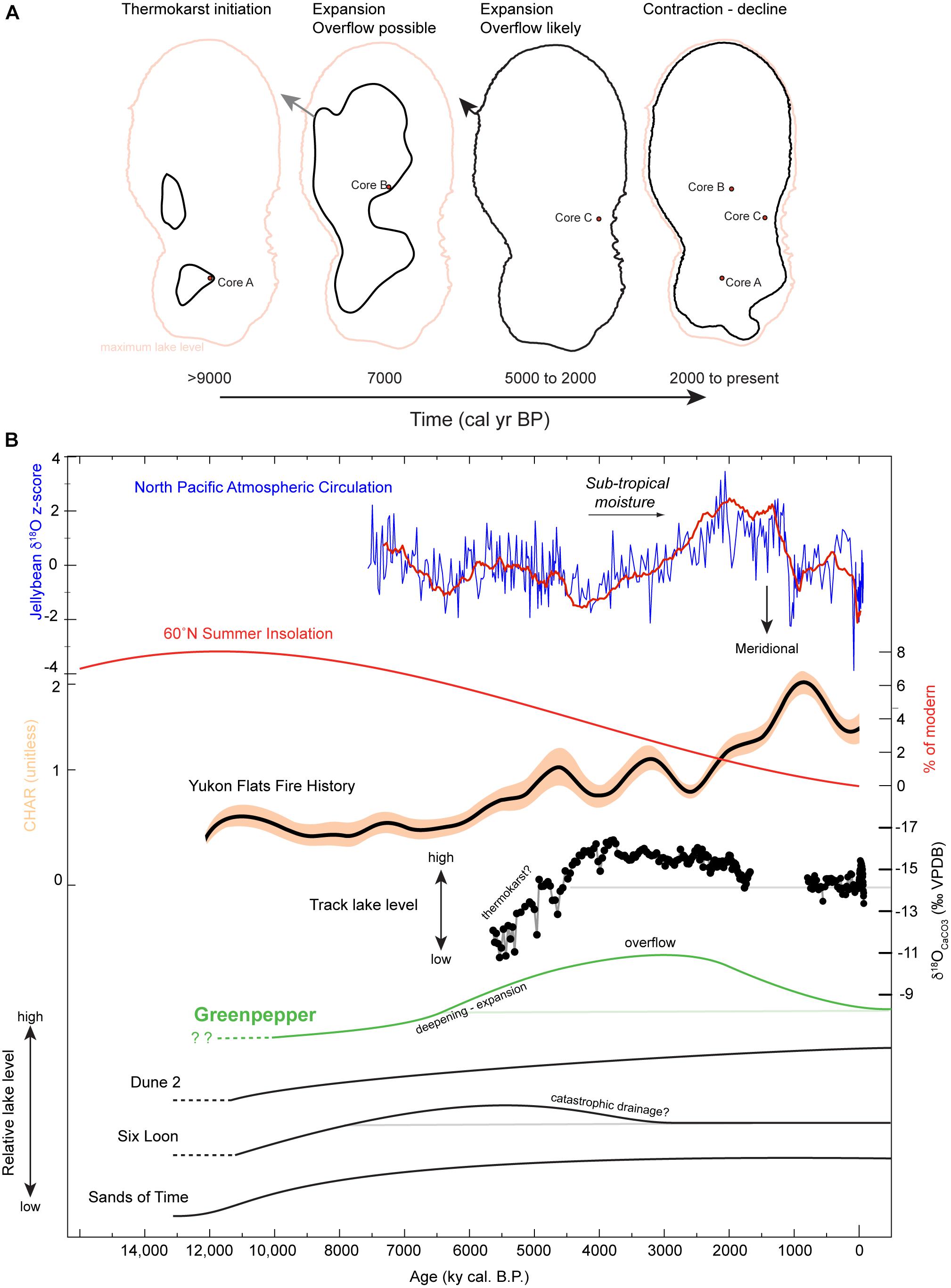
Figure 10. (A) Schematic of Greenpepper Lake shoreline evolution from ∼9000 cal yr BP to present. Faint orange outline of outlet elevation shoreline at 211.5 m is shown on each panel for context. (B) The evolution of loess plateau lakes on a relative lake level scale including Greenpepper (this study), and SoT, 6L, and D2 Lakes adapted from Edwards et al. (2016). Dashed lines represent periods of ‘trash’ layer development indicating thermokarst initiation and solid lines indicate periods of lacustrine sedimentation. The loess plateau lake levels are shown with the Jellybean Lake oxygen isotope record of North Pacific atmospheric circulation (z-score; Anderson et al., 2016), 60°N summer solar insolation (percent of modern), Yukon Flats fire history (normalized scale, Kelly et al., 2013), and Track Lake levels based on carbonate oxygen isotopes (Anderson et al., 2018).

At the core B location, active thermokarst is clearly evident by the lowermost 25 cm of sediment, which resembles a ‘trash’ layer composed of massive peaty silt, rich in woody material and charcoal of detrital origin and with high C/N and δ¹³C values (Figure 9). This material overlies stiff, inorganic silt with a pollen assemblage that includes damaged pre-Quaternary palynomorphs and damaged Picea grains. This is not a typical Holocene lake assemblage, and it suggests the presence of older sediment underlying the initial shallow lake; the lake is indicated by relatively high values of cell nets of the aquatic alga Pediastrum above ∼170 cm depth. Ages from terrestrial and aquatic material show that reversals and overlaps occur during the period between ∼6700 to 6400 cal yr BP and indicate that detrital material was deposited rapidly and chaotically at this time. The core B location on the 5-m bathymetric contour is used to estimate the expanding shoreline location of the lake by ∼7000 cal yr BP (Figure 10A).

The basal sequence at the core C location is composed of detrital ‘trash’ layers (Units V and IV), with 80 cm of dense, massive to crudely banded, poorly sorted silt, rich in peat, bryophytes and shells indicating some mass transport into the lake but negligible resuspension or mobilization of detrital sediment. Overlapping radiocarbon ages reflect rapid and chaotic deposition over the period ∼5400 to 4750 cal yr BP before a transition to re-worked shoreline facies took place. Comparison with ages of the ‘trash’ layers in core B indicates that shoreline expansion to the core C location occurred over a 1000 to 2000 year period between ∼7000 and 5000 cal yr BP (Figures 5, 10A).

Between ∼5000 and 2000 cal yr BP, the preservation of fine laminae in Units II of both core A and B (Figure 5) indicates a deeper water column where suboxic conditions led to fine laminae preservation at the sediment-water interface. The limnological measurements of the modern water column indicate that declines in temperature, conductivity, and dissolved oxygen between ∼4 and 6 m water depths resulted in some laminae preservation at 10 m (core A) and massive, mottled textures at 5 m (Core B). If oxyclines/thermoclines formed at depths similar to today following the stabilization of Greenpepper Lake’s shorelines by ∼5000 cal yr BP, then contrasting sedimentation above and below the boundary provides a means to estimate former lake levels from the sediment cores. Following this model, the fine laminae at core A (unit II) indicate water depths > 5m by ∼9 ka. Subsequent expansion and deepening is indicated by the charcoal age of 5845 cal yr BP within core A laminae (Unit II), which corresponds with core B laminae (Unit II) and the lake transition facies at core C (Unit III), and reflects the establishment of the near-modern Greenpepper bathymetry and shoreline by that time (Figure 5). Soon after rising lake levels by ∼5000 cal yr BP, surface overflow could have formed the stranded outflow channel. With an elevation of 211.5 m, the outflow channel requires lake levels ∼4 m higher than modern and water depths of ∼14, 9, and 6 m at the core A, B, and C, locations respectively (Figure 10A). It is also possible that earlier thaw-basin configurations could have led to surface overflow, although prominent downward thaw mechanisms for areas rich in ground ice (i.e., where lakes rapidly deepen) would suggest that this is not likely.

By ∼2000 cal yr BP, there was transition to massive or faintly banded sedimentation at the sediment-water interfaces at locations A and B and detrital re-working within Unit II at core C. These changes are consistent with lake-level declines that led to more frequent oxygenation of the hypolimnion and which have persisted to the present day. The lake-level lowering led to continuous littoral sedimentation at core C (Unit I), suggesting shoreline stability. A basin-wide change in Fe-sulfide redox balance and carbonate preservation at the sediment-water interface may also reflect increased hydraulic residence times. Lower lake levels are also supported by higher percentages of Cyperaceae, which dominate the shoreline of the lake today.

Holocene Thermokarst and Paleoclimate in the Yukon Flats

The reconstruction of Greenpepper Lake’s evolution suggests a thermokarst origin, likely as two adjacent small thaw ponds by ∼9000 cal yr BP that eventually coalesced and developed water depths > 5 m by ∼8000 cal yr BP. Lake-basin expansion and deepening through ∼5000 cal yr BP eventually led to bathymetric stabilization and the likelihood of full talik development (West and Plug, 2008). By this time, lake levels were also ∼4 m above the modern shoreline and the lake was either permanently or intermittently hydrologically open, with surface overflow occurring through the now-abandoned outflow channel. Beginning ∼2000 cal yr BP, there was further water loss and lake levels declined with water losses to near-modern levels; this led to the surficially closed hydrology of the lake today, the longer hydraulic residence times and significant water losses by evaporation.

Clear sedimentary evidence for Greenpepper Lake’s thermokarst initiation was not obtained but expansion by thermokarst is clearly shown by the basal parts of cores B and C. Basin formation at 6L and D2 lakes dates to the late glacial/early Holocene transition (∼13,000 to 9,000 cal yr BP), a period of widespread thermokarst across northern Siberia and Alaska attributed to post-glacial warming and effective moisture increases on a landscape vulnerable to thaw (Figure 10B; Walter Anthony et al., 2014; Edwards et al., 2016). With the expansion of Picea ∼9,500 cal yr BP (Kelly et al., 2013), permafrost would have been increasingly insulated by the development of moss-heath ground cover and thicker organic-rich soils (e.g., Gaglioti et al., 2014; Edwards et al., 2016). Thermokarst initiation at Greenpepper was probably in place by ∼10,000 cal yr BP, just before the expansion of Picea forest, although a definitive conclusion is not possible from our data. Currently, heterogeneous ground ice conditions in the loess uplands are observed to exert strong controls on the evolution of thermokarst. For instance, during deglaciation, ground ice may have been closer to the surface and thermokarst relatively quick to initiate. Now, particularly in areas with deeper depths to the tops of syngenetic wedges, thermokarst development may require more extreme disturbance to initiate. High charcoal concentration in the core B trash layer that dates to ∼ 7000 to 6000 cal yr BP may indicate fire-enhanced expansion of Greenpepper Lake. At this time, P. mariana, the most flammable species in Alaskan boreal forests, expanded regionally, and is reported to have driven late-Holocene increase in fire frequency (Figure 10B; Kelly et al., 2013).

Holocene reconstructions of interior Alaska’s water balance indicate increasing lake levels from the early to mid-Holocene, and positive Holocene maxima between ∼5000 and 3000 cal yr BP (Abbott et al., 2000; Barber and Finney, 2000). This wet period also broadly corresponds with our higher inferred lake levels at Greenpepper and at nearby Track Lake, a lower elevation site on the Yukon Flats (Figures 1A, 10B; Anderson et al., 2018). A similar pattern to Greenpepper – of high lake levels followed by partial drainage – may also have occurred ∼5000 to 4000 cal yr BP at 6L lake (Edwards et al., 2016). Other proxy records indicate that this was a period of high effective moisture throughout the northern interior region (Anderson et al., 2018 and references therein). High Greenpepper lake levels could reflect some combination of local declines in evaporative losses and increase in precipitation and, with establishment of deep groundwater-surface water connectivity following talik development, an increase in groundwater influx; all would contribute to an increase in regional-to-local water balance. Similar lake level declines at Greenpepper and Track lakes after ∼2000 cal yr BP strongly implicate regional climate mechanisms for reduced effective moisture. Water-balance declines are also apparent in proxy data from low elevations in the northern interior (Anderson et al., 2007; Bird et al., 2009; Clegg et al., 2011; Rodysill et al., 2018); these declines correspond with cooling temperatures reflected by alpine glacier advances (Barclay et al., 2009; Anderson et al., 2011), which coincide with changes in North Pacific atmospheric circulation (Figure 10B; Anderson et al., 2016).

The raised shorelines around the two partially filled lake basins north of Greenpepper also indicate previously higher lake levels (Figure 1B). Although not sampled or dated, these two basins share the same relict drainage that intersects Greenpepper, allowing the reasonable assumption that all three lakes overflowed concurrently. Analyses of the digital elevation model indicate an elevation of the overflow channels for the smaller northern lakes that resulted in their catastrophic drainage, whereas the raised relict outflow from Greenpepper did not. However, a subsurface hydrologic connection between Greenpepper and the down-gradient lakes could have facilitated sub-surface water loss if base levels lowered following their catastrophic drainage, although this hypothesis is not tested.

Wetter conditions in low-elevation regions of interior Alaska, such as those after ∼5000 and before 2000 cal yr BP, were most likely to have occured with patterns where North Pacific ocean-atmosphere dynamics, such as the position of the Aleutian Low, enabled moisture to reach interior Alaska from primary moisture sources to the southwest, without encountering major topographic barriers (described in detail in Anderson et al., 2005, 2007, 2011). These patterns also generally delivered warmer air to the region and reflect a late-Holocene shift in dominance to sub-tropical influences on Alaskan climate (Barron and Anderson, 2011; Anderson et al., 2016). Reversal of moisture patterns by ∼2000 cal yr BP may have been restricted to lower elevations in the interior, since the Gulf of Alaska region experienced increasing coastal moisture and high-elevation glacial advance at this time. The Jellybean Lake record of North Pacific circulation regimes indicates that after ∼2000 cal yr BP, intensified Aleutian Low activity led to enhanced meridional flow variability, which is supported by subsequent ice core studies in the Alaska Range and by regional lake synthesis (Steinman et al., 2014; Osterberg et al., 2017; Winski et al., 2017). By amplifying topographic rain-out, intensified meridional flow restricts moisture delivery to the interior, and, with alternating northerly Arctic flow, could result in more frequent colder and drier air masses.

Conclusion

This study provides further insight on the evolution of thermokarst and the direction of large-scale changes in effective moisture during the Holocene in the Yukon Flats of Interior Alaska. We have provided detailed documentation of early Holocene thermokarst, basin expansions and stabilization, and subsequent climate-driven lake level variations. Similarities between the late-Holocene moisture records from Greenpepper and Track Lakes lend additional support to previously proposed hypotheses for North Pacific circulation adjustments as a major control on effective moisture changes within interior Alaska during the late Quaternary (Edwards et al., 2001; Anderson et al., 2005; Fisher et al., 2008).

Widespread permafrost instability and thermokarst development in the loess uplands of the Yukon Flats was enhanced during the warm, moist post-glacial period (as compared with earlier cool/cold and dry periods). While thermokarst development slowed with the establishment of boreal forest, it did not cease. After lakes formed, their size and depth has likely been affected directly by atmospheric circulation pattern changes and fire disturbance and indirectly through changes of permafrost, ground ice and sub-surface hydrology. Thus, in a loess landscape characterized by discontinuous permafrost, changes in lakes and drainages are likely to be complex. Changes in lake level and water chemistry may be (but are not always) strongly linked to prevailing precipitation. Loess-upland lake systems characterize several regions of Alaska (Arp and Jones, 2008) and Siberia (Walter et al., 2007). This study provides a framework for future investigation of the high-frequency paleoclimatic and paleolimnological signals embedded in their lithology and sediment chemistry, such as the finely laminated sediments in Greenpepper Lake.

Author Contributions

LA conceived the project, collected samples and measurements, developed and interpreted the data, and wrote the manuscript. ME interpreted the pollen and charcoal data, provided background, and reviewed and edited the manuscript. MS collected the core samples, produced lithological descriptions, interpreted the aqueous geochemistry, and reviewed and edited the manuscript. BF collected the core samples, produced the carbon isotope data, and reviewed the manuscript. CL produced the pollen data.

Funding

This research is supported by the U.S. Geological Survey Land Change Science Program.

Conflict of Interest Statement

The authors declare that the research was conducted in the absence of any commercial or financial relationships that could be construed as a potential conflict of interest.

Acknowledgments

The USGS ScienceBase data release reference for this publication is https://doi.org/10.5066/P9O7255D. We would like to thank Nikki Guldager, the U.S. Fish and Wildlife Service Yukon Flats National Wildlife Refuge, and Jim Webster, who provided the air transportation and logistical support that made this research possible. LacCore at the University of Minnesota provided core scanning; Tom Guilderson at the Lawrence Livermore National Laboratory and Chad Wolack at the Institute for Arctic, Antarctic and Alpine Research (INSTAAR) at the University of Colorado Boulder, provided AMS radiocarbon ages; Dan Engstrom at the Science Museum of Minnesota provided ²¹⁰Pb analyses; Alisa Mast at the U.S. Geological Survey Colorado Water Science Center, provided water chemistry data; Million Hailemichael at the Idaho State University Stable Isotope Laboratory provided stable isotope data. We also would like to thank Paco VanSistine for assistance with imagery and GIS, Colin Penn for coulometric measurements, Jeff Honke for pollen slide preparation, Laura Strickland for macrofossil identification, Will Wenban for analyzing charcoal, and Jeremy Haven’s for assistance with figures. We appreciate assistance by Jessica Rodysill and the two journal reviewers for constructive criticisms and suggestions that served to significantly improve the manuscript. Any use of trade, firm, or product names is for descriptive purposes only and does not imply endorsement by the U.S. Government.

Supplementary Material

The Supplementary Material for this article can be found online at: https://www.frontiersin.org/articles/10.3389/feart.2019.00053/full#supplementary-material

References

Abbott, M. B., Finney, B. P., Edwards, M. E., and Kelts, K. R. (2000). Lake-level reconstructions and paleohydrology of Birch Lake, Central Alaska, based on seismic reflection profiles and core transects. Quat. Res. 53, 154–166. doi: 10.1006/qres.1999.2112