 Ludovic Huguet
 Hagay Amit
 Thierry Alboussière
- 1Department of Earth, Environmental, and Planetary Sciences, Case Western Reserve University, Cleveland, OH, United States
- 2CNRS, IRPHE, Aix Marseille Université, Centrale Marseille, Marseille, France
- 3Laboratoire de Planétologie et de Géodynamique, CNRS UMR 6112, Université de Nantes, Nantes, France
- 4UCBL, ENSL, CNRS, LGL-TPE, Université de Lyon, Villeurbanne, France
The convective state of the top of Earth's outer core is still under debate. Conflicting evidence from seismology and geomagnetism provides arguments for and against a thick stably stratified layer below the core-mantle boundary. Mineral physics and cooling scenarios of the core favor a stratified layer. However, a non-zero secular variation of the total geomagnetic energy on the core-mantle boundary is evidence for the presence of radial motions extending to the top of the core. We compare the secular variation of the total geomagnetic energy with the secular variation of the geomagnetic dipole intensity and tilt. We demonstrate that both the level of cancellations of the sources and sinks of the dipole intensity secular variation, as well as the level of cancellations of the sources and sinks of the dipole tilt secular variation, are either larger than or comparable to the level of cancellations of the sources and sinks of the total geomagnetic energy secular variation on the core-mantle boundary, indicating that the latter is numerically significant hence upwelling/downwelling reach the top of the core. Radial motions below the core-mantle boundary are either evidence for no stratified layer or to its penetration by various dynamical mechanisms, most notably lateral heterogeneity of core-mantle boundary heat flux.
1. Introduction
In the outer core of the Earth, the turbulent convective flow of an electrically conducting fluid drives the geodynamo. The geomagnetic field is the measurable consequence of this geodynamo. The main feature of the geomagnetic field is the dominance of the dipole component. Based on models of the geomagnetic field and its secular variation (SV) from ground and satellite observations (Jackson et al., 2000; Finlay et al., 2015, 2016b; Gillet et al., 2015), the dipole intensity has been decreasing rapidly (e.g. Gubbins, 1987; Olson and Amit, 2006; Finlay, 2008). The dipole decrease could be related to magnetic energy cascade (Amit and Olson, 2010) or non-local transfers from the dipole to high spherical harmonic degrees (Huguet and Amit, 2012). Inferring energy transfers at the top of the Earth's core may, therefore, provide important insights into the way the fluid flow at the top of the core distributes the geomagnetic energy. Huguet et al. (2016) developed a theoretical formalism for the magnetic to magnetic and kinetic to magnetic energy transfers just below the core-mantle boundary (CMB). They showed that the existence of kinetic to magnetic energy transfer corresponds to the presence of magnetic field stretching induced by upwelling/downwelling at the top of the core.
For decades, the existence of a stably stratified layer below the CMB has been a conundrum. Its origin (thermal or compositional), temporal evolution and the consequences for core dynamics and for the geodynamo are still puzzling. Several seismic studies suggested the presence of low P-waves velocity zone at the top of the Earth's core, which requires a lower density than the bulk of the outer core in order to remain stable (Helffrich and Kaneshima, 2010; Tang et al., 2015; Kaneshima, 2018). In contrast, Alexandrakis and Eaton (2010) did not find seismic evidence for stratification at the top of the core. Based on the observation of the SmKS waves which reflect below the CMB, Kaneshima (2018) argued that its thickness is about 450 km, larger than a previous estimate of about 300 km (Kaneshima and Helffrich, 2013). However, the new seismic model of Irving et al. (2018) explains the seismic observations without a slow and thick stable layer at the top of the outer core, that is consistent with a fully adiabatic outer core.
Several hypotheses were proposed to explain a chemical origin for a stratified region at the top of the Earth's core, but it still remains under debate. Diffusion of light elements from the mantle to the outer core could produce a thick layer (Gubbins and Davies, 2013), but it cannot explain the low seismic velocity profiles (Brodholt and Badro, 2017). During the early Earth, the release of a core impactor may explain the origin of a stably stratified layer (Landeau et al., 2016) if it has the right composition of light elements (Brodholt and Badro, 2017). Before the complete solidification of the lower mantle in the early Earth, interactions between a basal magma ocean and the top of the outer core may explain the formation of a light and seismically slow stratified layer (Brodholt and Badro, 2017).
Large outer core thermal conductivity corresponds to outer core heat flux partly conducted along the adiabat. In this case, the heat flux at the top of the core is sub-adiabatic and should lead to the formation of a thermal stably stratified layer while the deeper outer core convects (Gomi et al., 2013; Labrosse, 2015). However, the value of the thermal conductivity of iron under core pressure conditions is still under debate (Williams, 2018). Ab-initio calculations favor large core thermal conductivity (de Koker et al., 2012; Pozzo et al., 2012), whereas high pressure experiments have reported both large and low values (Gomi et al., 2013; Konôpková et al., 2016; Ohta et al., 2016). For example, the low outer core thermal conductivity proposed by Konôpková et al. (2016) would likely correspond to super-adiabatic conditions throughout the entire outer core.
Geomagnetic evidence for a stably stratified layer appears in the form of low geomagnetic SV at special points on the CMB where the field gradient is zero (Whaler, 1980). However, uncertainties on the exact locations of these points render such an analysis unreliable (Whaler and Holme, 2007). Magnetic, Archimedes and Coriolis (MAC) waves in a stratified layer are in agreement with the 60-year fluctuations of the geomagnetic dipole intensity over the historical era (Buffett, 2014; Buffett et al., 2016; Jaupart and Buffett, 2017). In contrast, intense geomagnetic flux patches at high latitudes and intensifying reversed flux patches below the South Atlantic are difficult to explain without the presence of upwelling/downwelling at the top of the core. Regional analysis of the SV at the CMB provides evidence for local magnetic flux concentrations, suggestive of the presence of fluid downwelling at the top of the core (Amit, 2014). Core flow inversions from geomagnetic SV exclude pure toroidal flow (Whaler, 1986) although the inclusion of a weak poloidal flow is sufficient to explain it (Lesur et al., 2015).
Convection in the deeper part of the outer core may penetrate a stably stratified layer (Takehiro and Lister, 2001; Takehiro, 2015; Takehiro and Sasaki, 2018). The length of penetration depends on the timescale and the length scale of the convective features of the outer core. Theoretical studies predicted a complete penetration of the stratified layer by the mean zonal flow (Takehiro and Sasaki, 2018). Outer core convection may also generate MAC waves in a stably stratified layer which include zonal radial flow (Buffett, 2014).
Recent studies attempted to reconcile evidence for a stratified layer from seismology and mineral physics with evidence for upwelling/downwelling from geomagnetism (Olson et al., 2017; Christensen, 2018). These studies relied on numerical dynamo simulations with an imposed stably stratified layer at the top of the shell and outer boundary heat flux heterogeneity. Here the main parameters controlling the competition between the stable layer and the boundary-driven convection are the layer thickness, the layer stability and the amplitude of CMB heat flux heterogeneity. The latter is estimated to be large enough (Nakagawa and Tackley, 2008) so that super-adiabatic conditions prevail where the CMB heat flux is large (Olson et al., 2017). The layer thickness and stability depend on the debated total CMB heat flux and core thermal conductivity. Olson et al. (2017) found for weak stratification that these local unstable regions stir the entire stable layer and lead to whole core convection. Their models are in agreement with the morphology of the time-average paleomagnetic field as long as the stable layer is thin. Christensen (2018) showed for strong stratification that the layer is not penetrated, and consequently, the magnetic field becomes too dipolar and too axisymmetric compared to the geomagnetic field (Christensen et al., 2010) due to a strong skin effect (Christensen, 2006; Nakagawa, 2011). In addition, such strong stratification would prevent the impact of CMB heterogeneity on the deeper core (e.g. by prescribing preferential inner core growth as proposed by Aubert et al., 2008). Mound et al. (2018) proposed that the CMB heterogeneity induces local stratification at low heat flux regions (rather than affecting a pre-existing global layer). These hot regions remain stable while in other parts convection reaches the CMB.
In this paper, we compare the temporal changes in the geomagnetic dipole with the temporal variations of the total geomagnetic energy on the CMB. In section 2 we recall the formalism of Huguet et al. (2016) for the energy transfer in 2D with radial magnetic field. Following Huguet et al. (2016), we compare the level of cancellations in the integrands of the SV of the total magnetic energy with that of the SV of the axial dipole but in much greater details. In addition, here we also compare the level of cancellations in the integrand of the SV of the total magnetic energy with that of the SV of the equatorial dipole. These ratios are computed based on the geomagnetic field and SV from several historical (Jackson et al., 2000; Gillet et al., 2015) and satellites (Finlay et al., 2015, 2016b) models. The results are presented in section 3. In section 4 we discuss our main results and their implications for the presence or absence of stratification at the top of the Earth's outer core.
2. Theory
2.1. Energy Transfers at the Top of the Core With Radial Magnetic Field
Here we recall the derivation of Huguet et al. (2016) for the magnetic to magnetic and kinetic to magnetic energy transfers at the top of the core. We show that non-zero SV of the total poloidal magnetic energy on the CMB requires kinetic to magnetic energy transfer. The existence of this energy transfer depends on the existence of upwelling/downwelling at the top of the core.
Our starting point is the radial magnetic induction equation in the frozen-flux limit (Roberts and Scott, 1965) just below the CMB (where, the radial velocity vanishes):
where Br is the radial magnetic field, dot denotes time derivative, is the velocity tangential to the spherical surface, and ∇h is the horizontal part of the differentiation operator. In Equation (1) the second term is the advection of the radial field by the tangential flow, the third term is the stretching of the field by the poloidal flow, and the first term is the SV. Multiplying (1) by Br/μ0 (where μ0 is the permeability of free space) gives
The first term in (2) is the integrand of the SV of the total (poloidal) magnetic energy:
where rc is the radius of the core and .
Next we split the stretching term in (2) into two halves:
The divergence theorem (or Green's theorem) for wrapped 2D surfaces like the spherical CMB gives trivially zero value for the integral of any divergence term. Therefore, integrating the sum of the second and third terms of (4) gives
We thus obtain
and
Based on (6–7), the local magnetic to magnetic energy transfer ėbb is due to the advection term plus half the stretching term, and the kinetic to magnetic energy transfer ėub is exclusively due to half the stretching term. Globally, the SV of the total (i.e., integrated over the CMB surface) poloidal magnetic energy is therefore due to kinetic to magnetic energy transfer only (8). This result is well-established for the 3D case, i.e., over the entire spherical shell (e.g. Alexakis et al., 2005a,b, 2007; Debliquy et al., 2005; Mininni et al., 2005; Carati et al., 2006; Mininni, 2011). Huguet et al. (2016) proved that it also holds for the 2D case.
2.2. Dipole Moment Changes
Here we recall the theory for the spatial contributions to dipole changes from Amit and Olson (2008). We describe the theory for both the axial and equatorial dipole components, which approximate the dipole intensity (Gubbins, 1987; Gubbins et al., 2006; Olson and Amit, 2006; Finlay et al., 2016a) and tilt (Amit and Olson, 2008), respectively.
The geomagnetic dipole moment vector is generally expressed in terms of an axial component mz and two components in the equatorial plane mx and my
The axial dipole moment can be written as
in terms of its integrand on the CMB ρz,
where a is the Earth's radius, is the axial dipole Gauss coefficient and the spherical coordinate system (ϕ, θ, r) denotes longitude, co-latitude, and radial distance, respectively.
Integrands can also be defined for the dipole moment components along the Cartesian x and y coordinates in the equatorial plane. The dipole moment integrands along longitudes 0°E and 90°E, respectively are
and the corresponding dipole moment components are
where and are the equatorial dipole Gauss coefficients.
The dipole components in the equatorial plane allow to define the equatorial component of the dipole moment as
in terms of the equatorial dipole moment density ρe on the CMB,
where is the longitude relative to that of the dipole axis. ϕ0(t) is the time-dependent longitude of the dipole axis given by Amit and Olson (2008)
Note that me is by definition positive (16). The dipole tilt angle θ0 can be written in terms of the axial and equatorial dipole moment components,
Finally, based on the above formalism, it is straightforward to write the SV of the dipole components in terms of spatial integrands. The time derivative of (11) gives
The time derivative of (17) gives
where the azimuthal angular velocity of the dipole axis is
2.3. Measures of the Level of Cancellations in the Integrands
In order to infer the significance of the values of the SV of the total geomagnetic energy, we define ratios of integrals with respect to their corresponding absolute integrals. Such integral ratios quantify the level of spatial cancellations at a given integral and may therefore assess the significance of the numerical values. Similar ratios were used to quantify the level of cancellations in the integrand of geomagnetic axial dipole change by meridional advection (Finlay et al., 2016a) and to calculate the regional level of cancellations in different SV contributions in numerical dynamos (Peña et al., 2016). Huguet et al. (2016) compared the level of cancellations of the SV of the total magnetic energy with those of the SV of the axial dipole. Here we recall these definitions and define a new quantity for the level of cancellations of the equatorial dipole.
Following (3) the ratio εe is defined by
This ratio represents the level of cancellations in the integrand of the SV of the total magnetic energy. For comparison, the ratio εmz represents the level of cancellations in the integrand of the SV of the axial dipole and is written
The dipole is the largest scale and the strongest component of the geomagnetic field. Its current intensity decrease is well-documented (Gubbins, 1987; Olson and Amit, 2006; Finlay, 2008; Finlay et al., 2016a; Metman et al., 2018). The ratio εmz therefore serves as a reference value to a level of cancellations that cannot be considered negligible.
In addition, following (23) we define the ratio εme which represents the level of cancellations in the integrand of the SV of the equatorial dipole
This new ratio defines an additional reference value for the level of cancellations that is significant.
3. Results
In this section, we plot the axial dipole SV (21), the equatorial dipole SV (23) and the total geomagnetic energy SV (3), all on the CMB, using various field models.
3.1. Changes in the Total Geomagnetic Energy
We use several geomagnetic field models. The gufm1 model in the historical era (1840–1990) (Jackson et al., 2000) was constructed from surface observatories and the MAGSAT satellite data. The COV-OBS.x1 model covers the historical era until present-day, including satellite data of the past two decades (1840–2020) (Gillet et al., 2015). COV-OBS.x1 is an ensemble of 100 models that accounts for data uncertainties. The CHAOS-5 (Finlay et al., 2015) and CHAOS-6 (Finlay et al., 2016b) models rely exclusively on recent high-quality satellite data (1997.1–2016 and 1997.1–2018, respectively). All models are expanded until spherical harmonic degree nmax = 14.
We start with an example of the radial geomagnetic field on the CMB (Figure 1A) and its SV (Figure 1B) which combine to produce the integrand of the SV of the total magnetic energy (Figure 1C), using the field model CHAOS-5 (Finlay et al., 2015) of the year 2015. The geomagnetic SV is dominated by small scales with numerous pairs of opposite sign structures that sum up by definition identically to zero. The integrand of the SV of the total geomagnetic energy is also dominated by pairs of opposite sign structures; However, the integrated outcome is different. At low latitudes of the Southern Hemisphere, several positive local contributions to the SV of the total geomagnetic energy appear below the Indian Ocean and West Africa, with their negative counterparts being much weaker. In addition, below Siberia a negative structure is sandwiched by two positive structures. Overall, there are more positive contributions than negative, i.e., the total geomagnetic energy is instantaneously increasing in this model.
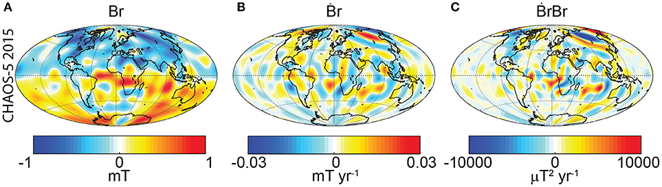
Figure 1. (A) Br, (B) , and (C) , all for the geomagnetic field model CHAOS-5 in the year 2015 (Finlay et al., 2015).
Figure 2 shows , the integrated SV of total magnetic energy, during the historical era. Non-zero values are observed, though at this stage it still remains to be demonstrated that these values are numerically significant. In the early period, the two field models differ significantly, possibly due to some spurious edge effects in COV-OBS.x1 (Metman et al., 2018, N. Gillet, personal communication). These edge effects are well known in comprehensive field models (e.g., Wardinski and Holme, 2006; Olsen et al., 2009; Gillet et al., 2013). However, the period over which these effects may last is unknown; It may depend on the modeling strategy. Between 1910 and 1990 both models exhibit increasing total geomagnetic energy with similar trends. Interestingly, starting from 1990 the value begins to decrease rapidly and around 2010 changes its sign giving decreasing total geomagnetic energy with time at present-day.
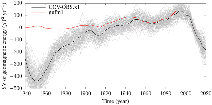
Figure 2. The SV of the total geomagnetic energy on the CMB as a function of time for gufm1 in the period 1840–1990 (red; Jackson et al., 2000) and COV-OBS.x1 in the period 1840–2020 (black; Gillet et al., 2015). Gray lines correspond to the ensemble of 100 models of COV-OBS.x1. Dashed horizontal green line denotes zero. Note that the SV of the total geomagnetic energy is in units of μT2yr−1.
3.2. Changes in the Geomagnetic Dipole
Figure 3 shows the time-evolution of the geomagnetic dipole and its temporal rate of change. Because the dipole is the most robust feature of the field, its uncertainty is the smallest and the 100 models of COV-OBS.x1 are practically identical to its mean. In addition, all three models (gufm1, COV-OBS.x1, and CHAOS-5) are in excellent agreement for the dipole. The axial dipole (Figure 3A) has been decreasing since 1840 (e.g., Gubbins, 1987; Gubbins et al., 2006; Olson and Amit, 2006; Finlay, 2008; Finlay et al., 2016a) and perhaps even further back in the past (Poletti et al., 2018). However, the rate of axial dipole decrease (Figure 3B) has been undulating (Olson and Amit, 2006; Buffett, 2014; Finlay et al., 2016a). The equatorial dipole (Figure 3C) and the tilt (Figure 3E) are highly correlated. Until 1960 very small tilt changes are observed, but since then the dipole axis is rapidly drifting poleward. This trend, noted a decade ago by Amit and Olson (2008), persists to present-day (Figures 3C,E). Figures 3D,F are also highly correlated and show that the poleward drift of the dipole tilt is steadily accelerating.
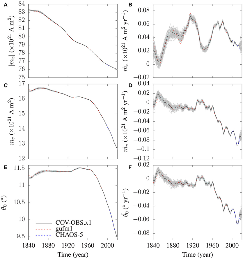
Figure 3. Geomagnetic dipole as a function of time for gufm1 (red dashed line; Jackson et al., 2000), COV-OBS.x1 (black solid line; Gillet et al., 2015) and CHAOS-5 (blue dashed line; Finlay et al., 2015). Gray lines correspond to the ensemble of 100 models of COV-OBS.x1. Absolute axial component |mz| (A), equatorial component me (C) and tilt θ0 (E) and time derivatives of axial component (B), equatorial component (D), and tilt (F).
The local contributions to the axial and equatorial dipole components are shown in Figure 4. The polarity of the geomagnetic field in the present chron is negative. Hence, normal flux patches, especially at high latitudes, provide dominant negative contributions to the axial dipole integrand, whereas reversed flux patches, in particular below the South Atlantic, provide positive contributions, that is, opposite to the dominant polarity (Gubbins, 1987; Gubbins et al., 2006; Olson and Amit, 2006; Terra-Nova et al., 2015; Metman et al., 2018). The equatorial dipole integrand is comprised of four quadrants separated by the equator and the two meridians 90 degrees east and west off the dipole longitude ϕ0 (Amit and Olson, 2008). The Northwest and Southeast quadrants provide positive contributions to me, whereas the Northeast and Southwest quadrants provide negative contributions. The high level of cancellations in Figure 4B reflects the small magnitude of me relative to mz. However, the positive contributions exceed the negative ones, yielding at present a tilt of ~10° of the dipole axis from the rotation axis (Figure 3E).
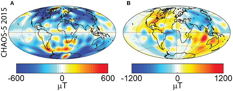
Figure 4. Geomagnetic dipole integrands for the axial mz (A) and equatorial me (B) components for the year 2015 of CHAOS-5 (Finlay et al., 2015).
3.3. Comparing Total Geomagnetic Energy and Dipole Changes
The integrands of (ρz in (20)), (ρe in (22)), and () are shown in Figure 5 for four snapshots. Visually, all three of these quantities exhibit multiple sources and sinks in all four snapshots. Quantitatively, is almost five times larger in 1940 than in 1900 (Figure 2). Indeed, fewer cancellations in in 1940 are seen, in particular, the positive strip along the longitude of central Asia (Figures 5I,F). Likewise, in 1980 when the dipole tilt was rapidly decreasing (Figures 3C–F), more positive ρe structures are observed, in particular, two long meridional strips below central Asia and Oceania (Figure 5E). In contrast, in 1900 and 1940 when the dipole tilt varied slowly (Figures 3C–F), the ρe distributions are much more balanced (Figures 5H,K). However, in order to quantitatively assess and compare the level of cancellations of the three integrands, we turn to the measures introduced in section 2.3.
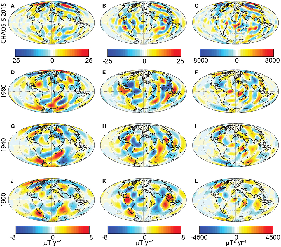
Figure 5. Integrands of (A,D,G,J), (B,E,H,K), and (C,F,I,L) for CHAOS-5 in 2015 (A–C) and gufm1 in 1900 (D–F), 1940 (G–I), and 1900 (J–L).
Figure 6 shows the evolution of the ratios εe (25), εmz (26), and εme (27) for the geomagnetic field models gufm1 (Jackson et al., 2000) and COV-OBS.x1 (Gillet et al., 2015). Note that the two field models are not overlapping, a consequence of the non-linearity of the ε quantities. The 100 models of COV-OBS.x1 provide an estimate of the error.
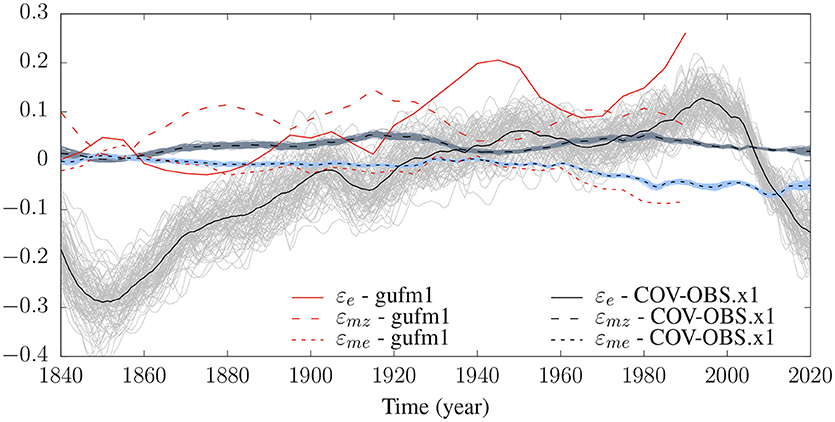
Figure 6. Evolution of the ratios εe (solid lines), εmz (dashed lines), and εme (dotted lines) using gufm1 (red lines) and the mean of COV-OBS.x1 (dark lines). The family of 100 COV-OBS.x1 models is presented in light, dark gray, and light blue solid lines for εe, εmz, and εme, respectively.
For gufm1, until ~ 1920 εmz was in general larger than εe, whereas after 1920 the latter was much larger. Until ~ 1960 εme was nearly zero and in general smaller than εmz and εe. This corresponds to the constant tilt period (Figures 3C-F; see also Amit and Olson, 2008; Amit et al., 2018). Since 1960, εme decreases in parallel to the decrease of the dipole tilt, with maximum absolute εme value in the last decade of the model. At the end of this period |εme| reaches a comparable value to |εmz|, both much lower than that of εe. At most times, however, the absolute values of εme in gufm1 are smaller than those of εe and εmz.
The ensemble of 100 models of COV-OBS.x1 show significant variability in εe, especially at earlier times, but for εmz and εme in practice the 100 models are identical to their respective mean values. This is to some extent expected because the uncertainty in COV-OBS.x1 is smallest for the dipole (Gillet et al., 2015). In COV-OBS.x1, εmz and εme exhibit similar trends as in gufm1 but with smaller amplitudes, especially for εmz. Overall εe exhibits large amplitude oscillations and its value is comparable to or larger than εmz and εme except for a few snapshots when εe changes sign (e.g., around 1940 and 2010). As in gufm1 εme is nearly zero until 1960 and decreasing thereafter, though its amplitude is smaller than in gufm1.
We proceed to further test the dependence of our results on the small scales of the geomagnetic field and its SV. In Figure 7 we show the ratios εe, εmz, and εme for four snapshots as a function of the truncation degree of spherical harmonic nmax. For the overlapping years εe shows significant differences between gufm1 and the mean of COV-OBS.x1 for nmax > 8 (as in Figure 6), whereas, for smaller nmax both models are in decent agreement. For all nmax values, εmz and εme are very similar in the two models. The three ε values approach asymptotic values with increasing resolution (Figure 7).
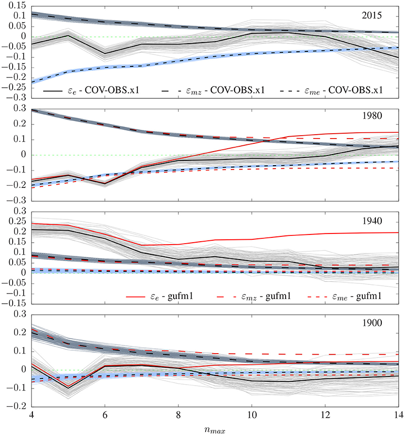
Figure 7. Ratios εe (solid lines), εmz (dashed lines), and εme (dotted lines) as a function of nmax for four snapshots using gufm1 (red, Jackson et al., 2000) and the mean of COV-OBS.x1 (black, Gillet et al., 2015). The family of 100 COV-OBS.x1 models is presented in light, dark gray, and light blue lines for εe, εmz and εme, respectively. Green line denotes the zero value.
For the year 1980 in gufm1, εe and εme are comparable for small nmax but εmz is larger. For large nmax, the absolute values of εmz and εme are comparable while εe is largest. In 1940 εe is by far the largest and εme is very small for all nmax values. In 1900 εmz is the largest for most nmax values (Figure 7).
The εe values of the ensemble of 100 models of COV-OBS.x1 include zero values for all years. Nevertheless, all ratios show an asymptotic behavior with increasing nmax, which provides evidence for the significance of the εe and values. The envelope of 100 models surrounds the mean values. For εe the envelope widens with increasing nmax, whereas for εmz and εme the corresponding envelopes are thin for all nmax values (Figure 7). In 2015 for low nmax the absolute εme is the largest, but at nmax = 13 the εe and εme of the mean of COV-OBS.x1 cross and at nmax = 14 in most of the 100 models εe is the largest. In 1980 for low nmax the absolute εmz is largest, whereas for large nmax the three ratios of the mean of COV-OBS.x1 are comparable with about half of the 100 models exhibiting largest εe values. In 1940 εe is by far the largest ratio, especially at low nmax. Finally, in 1900 for most nmax εe is the largest ratio (Figure 7).
Figures 8A,B show all ratios as functions of time and nmax respectively for the satellites era. With the full resolution during this period the absolute value of εme is the largest (Figures 8A). For small nmax, εe is much smaller than εmz and εme; increasing nmax gives εe comparable to εmz but still smaller than εme (Figures 8B). We also compared the results based on CHAOS-5 (Finlay et al., 2015) and CHAOS-6 (Finlay et al., 2016b). The results are practically identical for εmz and εme, whereas for εe some mild discrepancies exist. Finally, we note that the results for CHAOS-5 and CHAOS-6 (Figure 8A) differ from those for COV-OBS.x1 (Figure 6) in the overlapping period. This demonstrates the significance of the small-scale field and SV, which somewhat differ from one model to another, in the ϵe, ϵmz, and ϵme quantities.
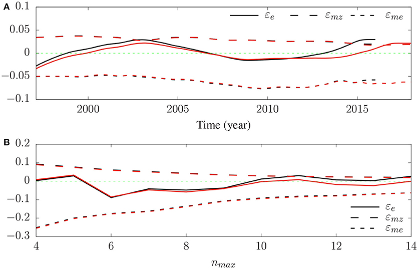
Figure 8. The ratios εe (solid lines), εmz (dashed lines), and εme (dotted lines) for the models CHAOS-5 (black ; Finlay et al., 2015) and CHAOS-6 (red ; Finlay et al., 2016b) as a function of time for nmax = 14 (A) and as a function of nmax for the year 2015 (B).
3.4. Can Magnetic Diffusion Explain the Changes in the Total Geomagnetic Energy?
The analysis above relies on the frozen-flux approximation, i.e., magnetic diffusion effects are assumed negligible compared to the effects of advection and stretching (Roberts and Scott, 1965). This approximation is supported by large estimates of the magnetic Reynolds number (e.g., Holme, 2015). However, the presence of a magnetic boundary layer at the top of the core may introduce a small radial length scale and significantly larger magnetic diffusion contributions to the SV than often considered (Gubbins, 1996; Amit and Christensen, 2008; Barrois et al., 2017). In addition, for global quantities such as the dipole (or the total magnetic energy), particular field-flow interactions might yield inefficient advection and hence large relative diffusive contribution (Olson and Amit, 2006; Finlay et al., 2016a).
Modeling magnetic diffusion SV from observations is problematic because the field inside the core is in general unknown. Amit and Christensen (2008) found in numerical dynamos a significant correlation between the patterns of tangential and radial magnetic SV. They proposed that intense magnetic flux patches on the outer boundary are concentrated by fluid downwellings which are the surface expressions of columnar helical vortices. Inside a flow column the tangential divergence is weaker, therefore the magnetic flux patch diffuses both tangentially and inwards, hence the correlation between tangential and radial diffusion. This model was recently confirmed by core flow re-analysis (Barrois et al., 2017) and joint inversion of magnetic and velocity fields (Barrois et al., 2018).
The complete radial induction equation at the top of the core, including magnetic diffusion, is written
where λ is magnetic diffusivity and r is the radial coordinate. The last two terms are radial and tangential diffusion respectively. According to the model of Amit and Christensen (2008)
and
where λ* is the effective magnetic diffusivity which accounts for radial diffusion. Because tangential diffusion is known from geomagnetic field models, (29) allows to model the full magnetic diffusion SV. With this magnetic diffusion term, (8) becomes
with the local diffusive contribution to Ėb given by
First we assess analytically the role of magnetic diffusion. Using the identities for tangential Laplacian and orthogonality of spherical harmonics, (32) can be rewritten as
where is the radial field of degree n and order m. Equation (33) indicates that, based on the model of Amit and Christensen (2008), diffusion would always decrease the total magnetic energy. Inspection of Figure 2 clearly shows that this is not the case. The total geomagnetic energy has increased for about a century. This proves that magnetic diffusion alone cannot explain the SV of the total geomagnetic energy.
However, can magnetic diffusion explain in part the Ėb trend? Next, we assess numerically the role of magnetic diffusion. Amit and Christensen (2008) extrapolated the magnitude of the core's effective magnetic diffusivity to λ* = 100−1000 m2 s−1, while the amount of diffusion in the solutions of Barrois et al. (2017) corresponds to λ* = 100−250 m2 s−1. In Figure 9 we compare the SV of the total geomagnetic energy vs. its diffusive contribution with a relatively low estimate of λ* = 100 m2 s−1. Clearly, the trends are distinctive. In summary, based on the model of Amit and Christensen (2008), magnetic diffusion is unlikely the origin of the SV of the total geomagnetic energy.
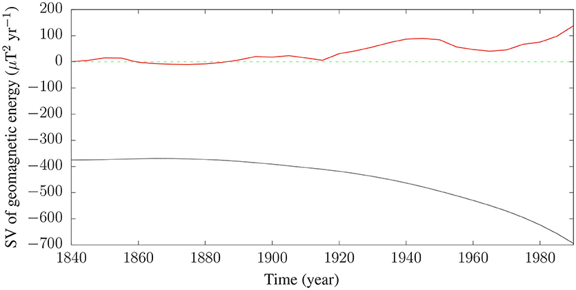
Figure 9. The SV of the total geomagnetic energy on the CMB as a function of time for gufm1 in the period 1840–1990 (red; Jackson et al., 2000) and its diffusive contribution with λ* = 100 m2 s−1 (black). The red line is the same as in Figure 2.
4. Discussion
In most cases εe is larger than εmz and εme, i.e., there are fewer cancellations in the integrand of the SV of the total geomagnetic energy. In some specific years, the εe curve crosses zero values in some models of the COV-OBS.x1 ensemble (Gillet et al., 2015). However, Figure 6 clearly indicates that it is likely that there are fewer cancellations in the spatial contributions to the SV of the total geomagnetic energy than in those of the SV of the axial and equatorial dipole components.
Obviously, a geomagnetic field and SV model characterized by poor spatial resolution might bias the results. Sensitivity tests for the role of small-scale field and SV (Figure 7) demonstrate once again that if the geomagnetic field models over the last century are robust then the level of cancellations in the integrand of the SV of the total geomagnetic energy is in most cases comparable to or smaller than the level of cancellations in the integrands of the SV of the axial and equatorial dipole components. An exception is the CHAOS-5 and CHAOS-6 field models which exhibit smallest cancellations in the integrand of the SV of the equatorial dipole (Figure 8A), but the short period covered by these models renders their interpretation statistically insignificant. The overall comparable or larger εe values are found in different field models, at most times and accounting for different small-scale contents. The latter test includes both the 100 models of COV-OBS.x1 (Gillet et al., 2015) as well as different truncations of field and SV models. For strongly truncated field and SV, dominance alternates in time among the three ε quantities. Asymptotic behavior with increasing nmax is encouraging. At present-day, according to the CHAOS-5 model (Finlay et al., 2015), the level of cancellations in the integrand of the SV of the total geomagnetic energy is comparable to that of the SV of the axial dipole, though the rapidly decelerating tilt results in the lowest level of cancellations for the SV of the equatorial dipole (Figure 8).
Interestingly, the evolution of me and εme exhibit similar trends, i.e., nearly constant until 1960 and rapidly decreasing since (see Figures 3, 6; Amit and Olson, 2008; Amit et al., 2018). This transition in me could in principle be due to the same distribution of but decrease in amplitude, or decrease in the level of cancellations. The first scenario involves no change in εme. We therefore conclude that the rapid tilt decrease since 1960 is related to genuine changes in the level of cancellations of .
Because the SV of the geomagnetic dipole is robust, we propose that the level of cancellations in its integrands can be considered as significant references. Our findings that the level of cancellations in the SV of the total geomagnetic energy is smaller than or comparable to those of the SV of the dipole components then indicates that the SV of the total geomagnetic energy is indeed non-zero. As we have shown, this supports the existence of upwelling/downwelling at the top of the core, in agreement with other inferences from the observed geomagnetic SV (Amit, 2014; Lesur et al., 2015).
The quantification of the effects of upwelling/downwelling at the top of the outer core is not trivial. In core flow inversions from geomagnetic SV the poloidal flow is usually coupled to the toroidal flow via some physical assumptions (e.g., Amit and Pais, 2013; Holme, 2015). Our formalism derived in section 2 may shed some light on the magnitude and size of upwelling/downwelling at the top of the core. The integrals of the SV of the total geomagnetic energy (3) and that of the kinetic to magnetic energy transfer (7) are identical. The associated integrands are not necessarily comparable. These integrals depend on the correlations between the various fields involved, which are reflected in the levels of cancellations. For example, if Br and are highly correlated or highly anti-correlated then ϵe will be close to unity, and conversely if Br and are nearly non-correlated then ϵe will approach zero. The same applies for the correlations between and the tangential divergence . However, because is positive and alternating upwelling/downwelling motions are present, it is likely that a similar high level of cancellations (or low correlations) appears in both. Assuming comparable integrands in (8) leads to the following evaluation for the magnitude of the tangential divergence
where B is a typical value of Br, Ḃ is a typical value of and δh is a typical upwelling/downwelling value. Using Ḃ ~2.5 μT yr−1 and B ~ 320 μT we get an estimated tangential divergence of δh ~1.5 century−1, comparable to previous estimates (see Olson et al. (2018) and references therein). This estimate represents a typical value, which of course may exhibit significant spatial variability, in particular in the presence of non-uniform thermal boundary conditions. If the amplitude of the CMB heat flux heterogeneity is on the order of unity (e.g., Nakagawa and Tackley, 2008; Olson et al., 2017; Christensen, 2018), the spatial variability of the large-scale persistent upwelling pattern may then reach 3 century−1. Next, the tangential divergence can be written as , where Up is the magnitude of the poloidal flow and L is the length scale of the upwelling/downwelling. As mentioned above the poloidal flow is difficult to estimate. However, in most core flow models, the toroidal flow is dominant. Assuming that the poloidal flow is an order of magnitude smaller than the toroidal, for a typical large-scale flow of 10 km/yr−1 (Finlay and Amit, 2011), Up = 1 km/yr−1 and the length scale of upwelling/downwelling is about 65 km, corresponding to spherical harmonic degree ℓ = 85. Without a magnetic field, Takehiro and Lister (2001) showed that columnar convection larger than 100 km can penetrate a thick stratified layer, whereas the presence of a magnetic field decreases the length scale for penetration to be larger than 1 km (Takehiro, 2015). If the upwelling/downwelling motions are associated with turbulent global convection in the entire core, the timescale of mixing of a pre-existing stably stratified layer corresponds to the thickness of the stratified layer divided by the radial motion velocity, which gives at least 450 years for a 450 km thickness layer. Then, the existence of a stably stratified layer depends on the existence of regeneration mechanisms or that the upwelling/downwelling are associated with MAC waves which will not mix the stratified layer with the rest of the outer core.
What are the consequences of our study for the possibility of stratification at the top of the core? No upwelling/downwelling corresponds to stable stratification. However, the opposite is not necessarily true; The existence of upwelling/downwelling at the top of the core does not necessarily exclude a stratified layer. Radial flow may penetrate a stably stratified layer if the convection columns are large enough (Takehiro and Lister, 2001) or at quasi-geostrophic conditions (Vidal and Schaeffer, 2015). Another proposed scenario is MAC waves (Buffett, 2014; Buffett et al., 2016; Jaupart and Buffett, 2017). However, the poloidal flow associated with MAC waves is very large scale and zonal, in contrast to the small scale poloidal flow that is strongly linked to the complex toroidal flow pattern found in most core flow models inferred from the geomagnetic SV (Bloxham and Jackson, 1991; Amit and Olson, 2006; Amit and Pais, 2013; Barrois et al., 2017). Alternatively, magnetohydrodynamics simulations show that zonal flows could completely penetrate a stably stratified layer (Takehiro, 2015; Takehiro and Sasaki, 2018). Once again, a zonal flow penetrating a stably stratified layer also seems too simplistic to explain the geomagnetic SV. It therefore seems plausible that the existence of a deep stably stratified layer would correspond to no upwelling/downwelling at the top of the core, i.e., no temporal change in the total magnetic energy on the CMB (Alexakis et al., 2005a). We conclude that our results serve as geomagnetic evidence against a deep stably stratified layer at the top of the core which is consistent with the most recent seismic model arguing in favor of a fully adiabatic outer core (Irving et al., 2018).
In summary, we demonstrated that independently of the geomagnetic field model used (gufm1, CHAOS-5, CHAOS-6, COV-OBS.x1), the spatial distribution of sources and sinks of the SV of the total geomagnetic energy is either less balanced than or as balanced as those of axial and equatorial dipole SV. The robustness of the geomagnetic dipole SV observations then indicates the existence of non-zero SV of the total geomagnetic energy. Because magnetic to magnetic energy transfer does not change the total geomagnetic SV (Huguet et al., 2016), kinetic to magnetic energy transfer should thus exist at the top of the core. Such a transfer relies on upwelling/downwelling motions at the top of the free stream. This suggests that a stratified layer at the top of the core is either shallow or destabilized by the e.g., lateral variability of CMB heat flux (Olson et al., 2017). Further exploration of the outer core using combined studies of geomagnetism, seismology, mineral physics, and numerical dynamos may shed light on the convective state of Earth's deep interior, in particular, the prospect of a stably stratified layer at the top of Earth's core.
Author Contributions
LH and HA designed this study. LH ran the calculations. LH, HA, and TA discussed the results and wrote the paper.
Funding
LH was supported by NASA grants NNX15AH31G. HA was supported by the Centre National d'Études Spatiales (CNES) and by the program PNP of INSU.
Conflict of Interest Statement
The authors declare that the research was conducted in the absence of any commercial or financial relationships that could be construed as a potential conflict of interest.
Acknowledgments
We thank Peter Olson and Maria L. Osete for their constructive reviews which helped to improve our paper.
References
Alexakis, A., Mininni, P., and Pouquet, A. (2005a). Imprint of large-scale flows on turbulence. Phys. Rev. Lett. 93:264503. doi: 10.1103/PhysRevLett.95.264503
Alexakis, A., Mininni, P., and Pouquet, A. (2005b). Shell to shell energy transfer in MHD. I. Steady state turbulence. Phys. Rev. E. 72:046301.doi: 10.1103/PhysRevE.72.046301t
Alexakis, A., Mininni, P., and Pouquet, A. (2007). Turbulent cascades, transfer, and scale interactions in magnetohydrodynamics. New J. Phys. 9, 1–20. doi: 10.1088/1367-2630/9/8/298
Alexandrakis, C., and Eaton, D. W. (2010). Precise seismic-wave velocity atop Earth's core: No evidence for outer-core stratification. Phys. Earth Planet. Inter. 180, 59–65.doi: 10.1016/j.pepi.2010.02.011
Amit, H. (2014). Can downwelling at the top of the Earth's core be detected in the geomagnetic secular variation? Phys. Earth Planet. Inter. 229, 110–121. doi: 10.1016/j.pepi.2014.01.012
Amit, H., and Christensen, U. (2008). Accounting for magnetic diffusion in core flow inversions from geomagnetic secular variation. Geophys. J. Int. 175, 913–924. doi: 10.1111/j.1365-246X.2008.03948.x
Amit, H., Coutelier, M., and Christensen, U. R. (2018). On equatorially symmetric and antisymmetric geomagnetic secular variation timescales. Phys. Earth Planet. Inter. 276, 190 – 201. doi: 10.1016/j.pepi.2017.04.009
Amit, H., and Olson, P. (2006). Time-average and time-dependent parts of core flow. Phys. Earth Planet. Inter. 155, 120–139. doi: 10.1016/j.pepi.2005.10.006
Amit, H., and Olson, P. (2008). Geomagnetic dipole tilt changes induced by core flow. Phys. Earth Planet. Inter. 166, 226–238. doi: 10.1016/j.pepi.2008.01.007
Amit, H., and Olson, P. (2010). A dynamo cascade interpretation of the geomagnetic dipole decrease. Geophys. J. Int. 181, 1411–1427. doi: 10.1111/j.1365-246X.2010.04596.x
Amit, H., and Pais, M. A. (2013). Differences between tangential geostrophy and columnar flow. Geophys. J. Int. 194, 145–157.doi: 10.1093/gji/ggt077
Aubert, J., Amit, H., Hulot, G., and Olson, P. (2008). Thermo-chemical wind flows couple Earth's inner core growth to mantle heterogeneity. Nature 454, 758–761. doi: 10.1038/nature07109
Barrois, O., Gillet, N., and Aubert, J. (2017). Contributions to the geomagnetic secular variation from a reanalysis of core surface dynamics. Geophys. J. Int. 211, 50–68. doi: 10.1093/gji/ggx280
Barrois, O., Hammer, M., Finlay, C., Martin, Y., and Gillet, N. (2018). Assimilation of ground and satellite magnetic measurements: inferenceof core surface magnetic and velocity field changes. Geophys. J. Int. 215, 695–712. doi: 10.1093/gji/ggy297
Bloxham, J., and Jackson, A. (1991). Fluid flow near the surface of the Earth's outer core. Rev. Geophys. 29, 97–120. doi: 10.1029/90RG02470
Brodholt, J., and Badro, J. (2017). Composition of the low seismic velocity E' layer at the top of Earth's core. Geophys. Res. Lett. 44, 8303–8310. doi: 10.1002/2017GL074261
Buffett, B. (2014). Geomagnetic fluctuations reveal stable stratification at the top of the Earth's core. Nature 507, 484–487. doi: 10.1038/nature13122
Buffett, B., Knezek, N., and Holme, R. (2016). Evidence for MAC waves at the top of Earth's core and implications for variations in length of day. Geophys. J. Int. 204, 1789–1800. doi: 10.1093/gji/ggv552
Carati, D., Debliquy, O., Knaepen, B., Teaca, B., and Verma, M. (2006). Energy transfers in forced MHD turbulence. J. Turb. 7:51. doi: 10.1080/14685240600774017
Christensen, U. (2018). Geodynamo models with a stable layer and heterogeneous heat flow at the top of the core. Geophys. J. Int. 215, 1338–1351. doi: 10.1093/gji/ggy352
Christensen, U. R. (2006). A deep dynamo generating Mercury's magnetic field. Nature 444:1056. doi: 10.1038/nature05342
Christensen, U. R., Aubert, J., and Hulot, G. (2010). Conditions for earth-like geodynamo models. Earth Planet. Sci. Lett. 296, 487–496. doi: 10.1016/j.epsl.2010.06.009
de Koker, N., Steinle-Neumann, G., and Vlček, V. (2012). Electrical resistivity and thermal conductivity of liquid Fe alloys at high P and T, and heat flux in Earth's core. Proc. Natl. Acad. Sci. U.S.A. 109, 4070–4073. doi: 10.1073/pnas.1111841109
Debliquy, O., Verma, M. K., and Carati, D. (2005). Energy fluxes and shell-to-shell transfers in three-dimensional decaying magnetohydrodynamic turbulence. Phys. Plas. 12:042309. doi: 10.1063/1.1867996
Finlay, C. (2008). Historical variation of the geomagnetic axial dipole. Phys. Earth Planet. Inter. 170, 1–14. doi: 10.1016/j.pepi.2008.06.029
Finlay, C., and Amit, H. (2011). On flow magnitude and field-flow alignment at Earth's core surface. Geophys. J. Int. 186, 175–192. doi: 10.1111/j.1365-246X.2011.05032.x
Finlay, C. C., Aubert, J., and Gillet, N. (2016a). Gyre-driven decay of the Earth's magnetic dipole. Nat. Commun. 7:10422. doi: 10.1038/ncomms10422
Finlay, C. C., Olsen, N., Kotsiaros, S., Gillet, N., and Tøffner-Clausen, L. (2016b). Recent geomagnetic secular variation from Swarm and ground observatories as estimated in the CHAOS-6 geomagnetic field model. Earth Plan. Space 68:112. doi: 10.1186/s40623-016-0486-1
Finlay, C. C., Olsen, N., and Tøffner-Clausen, L. (2015). DTU candidate field models for IGRF-12 and the CHAOS-5 geomagnetic field model. Earth Plan. Space 67:114. doi: 10.1186/s40623-015-0274-3
Gillet, N., Barrois, O., and Finlay, C. C. (2015). Stochastic forecasting of the geomagnetic field from the COV-OBS. x1 geomagnetic field model, and candidate models for IGRF-12. Earth Plan. Space 67:71. doi: 10.1186/s40623-015-0225-z
Gillet, N., Jault, D., Finlay, C., and Olsen, N. (2013). Stochastic modeling of the Earth's magnetic field: Inversion for covariances over the observatory era. Geochem. Geophys. Geosyst. 14, 766–786. doi: 10.1002/ggge.20041
Gomi, H., Ohta, K., Hirose, K., Labrosse, S., Caracas, R., Verstraete, M. J., and Hernlund, J. W. (2013). The high conductivity of iron and thermal evolution of the Earth's core. Phys. Earth Plan. Inter. 224, 88–103. doi: 10.1016/j.pepi.2013.07.010
Gubbins, D. (1996). A formalism for the inversion of geomagnetic data for core motions with diffusion. Phys. Earth Plan. Inter. 98, 193–206.
Gubbins, D., and Davies, C. (2013). The stratified layer at the core-mantle boundary caused by barodiffusion of oxygen, sulphur and silicon. Phys. Earth Plan. Inter. 215, 21–28. doi: 10.1016/j.pepi.2012.11.001
Gubbins, D., Jones, A., and Finlay, C. (2006). Fall in Earth's magnetic field is erratic. Science 312, 900–902. doi: 10.1126/science.1124855
Helffrich, G., and Kaneshima, S. (2010). Outer-core compositional stratification from observed core wave speed profiles. Nature 468, 807–810. doi: 10.1038/nature09636
Holme, R. (2015). “8.04 - Large-Scale Flow in the Core,”. in Treatise on Geophysics (2nd Edition) ed G. Schubert (Oxford: Elsevier), 91–113.
Huguet, L., and Amit, H. (2012). Magnetic energy transfer at the top of the Earth's core. Geophys. J. Int. 190, 856–870. doi: 10.1111/j.1365-246X.2012.05542.x
Huguet, L., Amit, H., and Alboussière, T. (2016). Magnetic to magnetic and kinetic to magnetic energy transfers at the top of the Earth's core. Geophys. J. Int. 207, 934–948. doi: 10.1093/gji/ggw317
Irving, J. C., Cottaar, S., and Lekić, V. (2018). Seismically determined elastic parameters for earths outer core. Sci. Adv. 4:eaar2538. doi: 10.1126/sciadv.aar2538
Jackson, A., Jonkers, A., and Walker, M. (2000). Four centuries of geomagnetic secular variation from historical records. Phil. Trans. R. Soc. Lond. A358, 957–990. doi: 10.1098/rsta.2000.0569
Jaupart, E., and Buffett, B. (2017). Generation of MAC waves by convection in Earth's core. Geophys. J. Int. 209, 1326–1336. doi: 10.1093/gji/ggx088
Kaneshima, S. (2018). Array analyses of SmKS waves and the stratification of Earth's outermost core. Phys. Earth Plan Inter. 276, 234–246. doi: 10.1016/j.pepi.2017.03.006
Kaneshima, S., and Helffrich, G. (2013). Vp structure of the outermost core derived from analysing large-scale array data of SmKS waves. Geophys. J. Int. 193, 1537–1555. doi: 10.1093/gji/ggt042
Konôpková, Z., McWilliams, R. S., Gómez-Pérez, N., and Goncharov, A. F. (2016). Direct measurement of thermal conductivity in solid iron at planetary core conditions. Nature 534, 99–101. doi: 10.1038/nature18009
Labrosse, S. (2015). Thermal evolution of the core with a high thermal conductivity. Phys. Earth Plan. Inter. 247, 36–55. doi: 10.1016/j.pepi.2015.02.002
Landeau, M., Olson, P., Deguen, R., and Hirsh, B. H. (2016). Core merging and stratification following giant impact. Nat. Geosci. 9, 786–789. doi: 10.1038/ngeo2808
Lesur, V., Whaler, K., and Wardinski, I. (2015). Are geomagnetic data consistent with stably stratified flow at the core–mantle boundary? Geophys. J. Int. 201, 929–946. doi: 10.1093/gji/ggv031
Metman, M., Livermore, P., and Mound, J. (2018). The reversed and normal flux contributions to axial dipole decay for 1880”2015. Phys. Earth Plan Inter. 276, 106 – 117. doi: 10.1016/j.pepi.2017.06.007
Mininni, P., Alexakis, A., and Pouquet, A. (2005). Shell-to-shell energy transfer in magnetohydrodynamics. II. Kinematic dynamo. Phys. Rev. E 72:046302. doi: 10.1103/PhysRevE.72.046302
Mininni, P. D. (2011). Scale interactions in magnetohydrodynamic turbulence. Ann. Rev. Fluid Mechan. 43, 377–397. doi: 10.1146/annurev-fluid-122109-160748
Mound, J., Davies, C. J., Rost, S., and Aurnou, J. M. (2018). The apparent stratification at the top of earth's liquid core. EarthArXiv. doi: 10.31223/osf.io/dvfjp
Nakagawa, T. (2011). Effect of a stably stratified layer near the outer boundary in numerical simulations of a magnetohydrodynamic dynamo in a rotating spherical shell and its implications for Earth's core. Phys. Earth Plan. Inter., 187, 342–352. doi: 10.1016/j.pepi.2011.06.001
Nakagawa, T., and Tackley, P. (2008). Lateral variations in CMB heat flux and deep mantle seismic velocity caused by a thermal-chemical-phase boundary layer in 3D spherical convection. Earth Planet. Sci. Lett. 271, 348–358. doi: 10.1016/j.epsl.2008.04.013
Ohta, K., Kuwayama, Y., Hirose, K., Shimizu, K., and Ohishi, Y. (2016). Experimental determination of the electrical resistivity of iron at Earth's core conditions. Nature 534, 95–98. doi: 10.1038/nature17957
Olsen, N., Mandea, M., Sabaka, T. J., and Tøffner-Clausen, L. (2009). CHAOS-2”a geomagnetic field model derived from one decade of continuous satellite data. Geophys. J. Int. 179, 1477–1487. doi: 10.1111/j.1365-246X.2009.04386.x
Olson, P., and Amit, H. (2006). Changes in earth's dipole. Naturwissenschaften 93, 519–542. doi: 10.1007/s00114-006-0138-6
Olson, P., Landeau, M., and Reynolds, E. (2017). Dynamo tests for stratification below the core-mantle boundary. Phys. Earth Plan Inter. 271, 1–18. doi: 10.1016/j.pepi.2017.07.003
Olson, P., Landeau, M., and Reynolds, E. (2018). Outer core stgh latitude structure of the geomagnetic field. Frontiers. Front. Earth Sci. 6:140. doi: 10.3389/feart.2018.00140
Peña, D., Amit, H., and Pinheiro, K. J. (2016). Magnetic field stretching at the top of the shell of numerical dynamos. Earth Plan Space 68:78. doi: 10.1186/s40623-016-0453-x
Poletti, W., Biggin, A. J., Trindade, R. I., Hartmann, G. A., and Terra-Nova, F. (2018). Continuous millennial decrease of the Earth's magnetic axial dipole. Phys. Earth Plan Inter. 274, 72–86. doi: 10.1016/j.pepi.2017.11.005
Pozzo, M., Davies, C., Gubbins, D., and Alfè, D. (2012). Thermal and electrical conductivity of iron at Earth's core conditions. Nature 485, 355–358. doi: 10.1038/nature11031
Roberts, P., and Scott, S. (1965). On analysis of the secular variation, 1, A hydromagnetic constraint: Theory. J. Geomagn. Geoelectr. 17, 137–151.
Takehiro, S.-I. (2015). Penetration of alfvén waves into an upper stably-stratified layer excited by magnetoconvection in rotating spherical shells. Phys. Earth Plan Inter. 241, 37–43. doi: 10.1016/j.pepi.2015.02.005
Takehiro, S.-I., and Lister, J. R. (2001). Penetration of columnar convection into an outer stably stratified layer in rapidly rotating spherical fluid shells. Earth Planet. Sci. Lett. 187, 357–366. doi: 10.1016/S0012-821X(01)00283-7
Takehiro, S.-I., and Sasaki, Y. (2018). Penetration of steady fluid motions into an outer stable layer excited by mhd thermal convection in rotating spherical shells. Phys. Earth Plan. Inter. 276, 258–264. doi: 10.1016/j.pepi.2017.03.001
Tang, V., Zhao, L., and Hung, S.-H. (2015). Seismological evidence for a non-monotonic velocity gradient in the topmost outer core. Sci. Rep. 5:8613. doi: 10.1038/srep08613
Terra-Nova, F., Amit, H., Hartmann, G. A., and Trindade, R. I. (2015). The time dependence of reversed archeomagnetic flux patches. J. Geophys. Res. 120, 691–704. doi: 10.1002/2014JB011742
Vidal, J., and Schaeffer, N. (2015). Quasi-geostrophic modes in the Earth's fluid core with an outer stably stratified layer. Geophys. J. Int. 202(3):2182–2193. doi: 10.1093/gji/ggv282
Wardinski, I., and Holme, R. (2006). A time-dependent model of the Earth's magnetic field and its secular variation for the period 1980–2000. J. Geophys. Res. 111:B12101. doi: 10.1029/2006JB004401
Whaler, K. (1986). Geomagnetic evidence for fluid upwelling at the core-mantle boundary. Geophys. J. R. Astr. Soc. 86, 563–588.
Whaler, K., and Holme, R. (2007). Consistency between the flow at the top of the core and the frozen-flux approximation. Earth Plan. Space 59, 1219–1229. doi: 10.1186/BF03352070
Keywords: geodynamo, stratification, outer core, magnetic field, core-mantle boundary, secular variation
Citation: Huguet L, Amit H and Alboussière T (2018) Geomagnetic Dipole Changes and Upwelling/Downwelling at the Top of the Earth's Core. Front. Earth Sci. 6:170. doi: 10.3389/feart.2018.00170
Received: 08 June 2018; Accepted: 28 September 2018;
Published: 18 October 2018.
Edited by:
Joshua M. Feinberg, University of Minnesota Twin Cities, United StatesReviewed by:
Peter Olson, Johns Hopkins University, United StatesMaria Luisa Osete, Complutense University of Madrid, Spain
Copyright © 2018 Huguet, Amit and Alboussière. This is an open-access article distributed under the terms of the Creative Commons Attribution License (CC BY). The use, distribution or reproduction in other forums is permitted, provided the original author(s) and the copyright owner(s) are credited and that the original publication in this journal is cited, in accordance with accepted academic practice. No use, distribution or reproduction is permitted which does not comply with these terms.
*Correspondence: Ludovic Huguet, aHVndWV0QGlycGhlLnVuaXYtbXJzLmZy